Learn AI Prediction & Neural Networks: From Math to Machine
Goal: Deeply understand how machines “learn” by building the mathematical engines from scratch. You will move beyond “import torch” to understanding tensors, gradients, backpropagation, and optimization algorithms at the byte level. By the end, you will have built your own deep learning library and deployed production-ready models for fraud detection and computer vision.
Why Under-the-Hood AI Matters
In the modern era, it’s easy to download a pre-trained model, run three lines of Python, and call yourself an AI engineer. But when the model hallucinates, when it overfits, or when you need to run inference on an embedded device with 128KB of RAM, “black box” knowledge fails.
Understanding the calculus and linear algebra behind neural networks isn’t just academic—it’s the difference between an operator and an engineer. The pioneers of AI (Hinton, LeCun, Bengio) didn’t just use libraries; they invented the mathematical structures that power them. To master AI, you must build the brain before you use it.
Core Concept Analysis
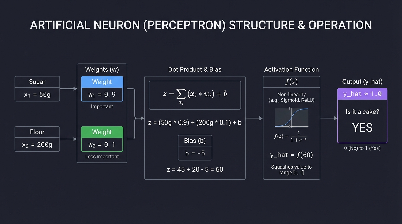
1. The Artificial Neuron (The Atom)
At its simplest, a neuron is just a filter. It takes inputs, weighs their importance, adds a bias (threshold), and decides whether to “fire” (activate).
      Inputs (x)        Weights (w)
    ┌──────────┐       ┌──────────┐
    │  Sugar   │──────►│   0.9    │ (Important)
    ├──────────┤       ├──────────┤
    │  Flour   │──────►│   0.1    │ (Less important)
    └──────────┘       └──────────┘
           │                 │
           ▼                 ▼
      Dot Product ( Σ x * w ) + Bias (b)
           │
           ▼
    ┌──────────────────────────────┐
    │    Activation Function f(z)  │  ◄── Non-linearity (Sigmoid/ReLU)
    └──────────────┬───────────────┘
                   │
                   ▼
             Output (y_hat)
        (Probability: "Is it a cake?")
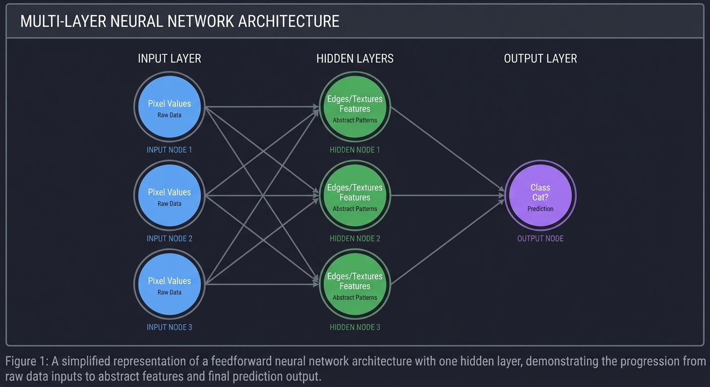
2. The Network (The Molecule)
One neuron makes a line. Many neurons make a shape. Layers of neurons make a thought. Deep learning is essentially function approximation: finding a complex mathematical function $F(x)$ that maps inputs to outputs.
    Input Layer       Hidden Layers (Features)      Output Layer
    (Raw Data)        (Abstract Patterns)           (Prediction)

       O ──┐             O ──┐
           │             │   │
       O ──┼────────────►O ──┼──────────────────────► O  (Cat?)
           │             │   │
       O ──┘             O ──┘
    Pixel Values      Edges/Textures                 Class
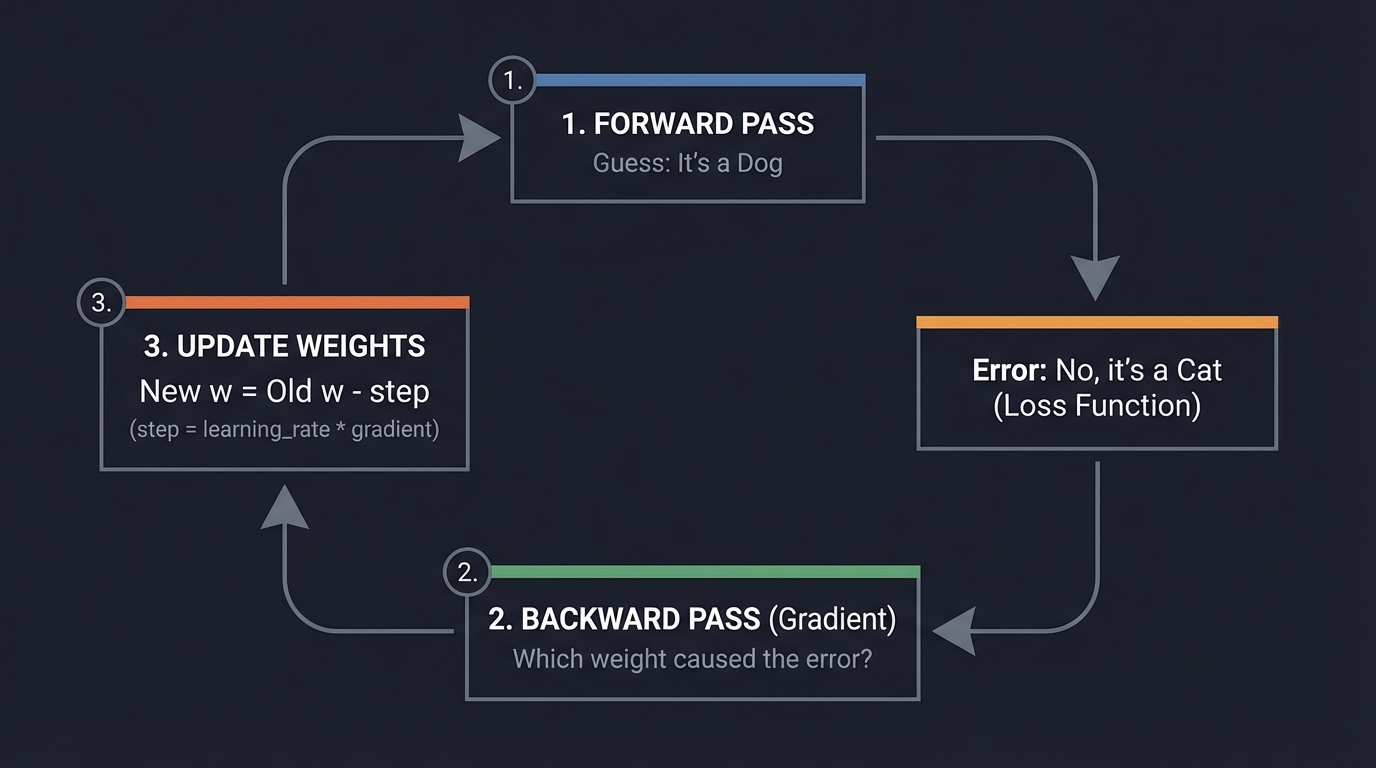
3. The Learning Cycle (The Engine)
How does it get smart? By making mistakes and correcting them. This is Gradient Descent.
    1. FORWARD PASS  ──────────►  Guess: "It's a Dog"
                                        │
                                        ▼
                                  Error: "No, it's a Cat" (Loss Function)
                                        │
    3. UPDATE WEIGHTS ◄─────────  2. BACKWARD PASS (Gradient)
       (New w = Old w - step)        "Which weight caused the error?"
4. Backpropagation (The Chain Rule)
This is the magic. We use Calculus (the Chain Rule) to calculate the “blame” for the error back through the network, layer by layer.
\[\frac{\partial Loss}{\partial w} = \frac{\partial Loss}{\partial output} \times \frac{\partial output}{\partial hidden} \times \frac{\partial hidden}{\partial w}\]Concept Summary Table
| Concept Cluster | What You Need to Internalize |
|---|---|
| Tensors & Dot Products | Everything is a matrix multiplication. The speed of AI comes from linear algebra efficiency. |
| Loss Functions | The “scorecard.” MSE for regression, Cross-Entropy for classification. It defines what “bad” looks like. |
| Gradient Descent | The “walker.” We are trying to find the lowest point in a valley (minimum loss) by taking small steps downhill. |
| Backpropagation | The “blame game.” Distributing the error correction backward to update every single connection weight. |
| Overfitting | Memorizing the data instead of learning patterns. Like a student who memorizes the answers but fails the test. |
Deep Dive Reading by Concept
| Concept | Book & Chapter |
|---|---|
| Foundations | “Deep Learning” by Goodfellow, Bengio, Courville — Ch. 2: “Linear Algebra” |
| Neural Networks | “Neural Networks and Deep Learning” by Michael Nielsen — Ch. 1: “Using neural nets to recognize handwritten digits” |
| Backpropagation | “Grokking Deep Learning” by Andrew Trask — Ch. 4-5: “Gradient Descent & Backpropagation” |
| Optimization | “Deep Learning” by Goodfellow — Ch. 8: “Optimization for Training Deep Models” |
| CNNs | “Deep Learning with Python” by François Chollet — Ch. 5: “Deep Learning for Computer Vision” |
Essential Reading Order
- Foundation (Week 1):
- Grokking Deep Learning Ch. 1-3 (The math of learning)
- Neural Networks and Deep Learning Ch. 1 (Perceptrons)
Project List
Project 1: The “Manual” Neuron
- File:
AI_PREDICTION_AND_NEURAL_NETWORKS_DEEP_DIVE.md - Main Programming Language: Python (Pure, NO NumPy yet)
- Alternative Programming Languages: C, Rust
- Coolness Level: Level 2: Practical but Forgettable
- Business Potential: 1. The “Resume Gold” (Educational)
- Difficulty: Level 1: Beginner
- Knowledge Area: Artificial Neurons / Logic Gates
- Software or Tool: Python Standard Library
- Main Book: “Grokking Deep Learning” by Andrew Trask
What you’ll build: A purely manual implementation of a Perceptron (single neuron) that “learns” to act as an AND/OR logic gate by adjusting two weight variables and a bias variable over thousands of iterations.
Why it teaches the Neuron: You cannot hide behind matrix multiplication here. You will write the code output = (input1 * weight1) + (input2 * weight2) + bias and manually implement the update rule. You will see exactly how numbers change to “learn” logic.
Core challenges you’ll face:
- Implementing the step activation function
- Calculating the error (Difference between expected and actual)
- The Delta Rule: Updating weights based on error size
- Converging on a solution that works for all truth table inputs
Key Concepts:
- Perceptron Update Rule: “Neural Networks and Deep Learning” Ch. 1 - Nielsen
- Linear Separability: Why a single neuron cannot solve XOR.
Difficulty: Beginner Time estimate: Weekend Prerequisites: Basic Python, high school algebra.
Real World Outcome
You’ll run a script that starts with random garbage weights (guessing randomly) and prints its “learning process” until it perfectly mimics a logic gate.
Example Output:
$ python manual_neuron.py --gate OR

Initial Weights: w1=0.2, w2=-0.5, b=0.1
---------------------------------------
Epoch 1: Input=[0,1] Target=1 Predicted=0 Error=1 -> UPDATING weights
Epoch 2: Input=[1,0] Target=1 Predicted=0 Error=1 -> UPDATING weights
...
Epoch 45: Solved!
Final Weights: w1=1.1, w2=1.1, b=-0.1

Testing Model:
[0, 0] -> 0 (Correct)
[0, 1] -> 1 (Correct)
[1, 0] -> 1 (Correct)
[1, 1] -> 1 (Correct)
The Core Question You’re Answering
“How can multiplying numbers lead to ‘decisions’?”
Before coding, realize that “making a decision” in AI is just drawing a line. If the weighted sum is above the line, it’s Yes; below, it’s No. You are building a machine that finds that line.
Concepts You Must Understand First
- Dot Product: Multiplying inputs by weights and summing them.
- Error Calculation:
Error = Target - Prediction. - Learning Rate: Why we multiply the error by a small number (alpha) before updating.
Project 2: The Gradient Descent Visualizer
- File:
AI_PREDICTION_AND_NEURAL_NETWORKS_DEEP_DIVE.md - Main Programming Language: Python (Matplotlib + NumPy)
- Coolness Level: Level 3: Genuinely Clever
- Difficulty: Level 2: Intermediate
- Knowledge Area: Optimization / Calculus
- Main Book: “Deep Learning” by Goodfellow - Ch. 4
What you’ll build: A CLI/GUI tool where you define a mathematical function (like a bowl shape: $z = x^2 + y^2$), start a “ball” at a random point, and visualize it rolling down to the bottom (minimum) using the gradient descent algorithm.
Why it teaches Optimization: Neural networks are just complex functions with millions of variables. Training them is just finding the minimum. This project makes the abstract concept of “descending the loss surface” concrete and visual.
Core challenges you’ll face:
- Calculating partial derivatives (the gradient) manually for your function.
- Implementing the update step:
x_new = x_old - (learning_rate * gradient). - Handling “overshooting” (learning rate too high) or “stalling” (learning rate too low).
- Visualizing 3D surfaces or 2D contour maps.
Key Concepts:
- Partial Derivatives: Calculus I/II refresher.
- The Gradient Vector: The direction of steepest ascent.
- Learning Rate/Step Size: The hyperparameters of training.
Difficulty: Intermediate Time estimate: Weekend Prerequisites: Calculus basics (Derivatives).
Real World Outcome
A visual plot (or ASCII animation) showing a point moving closer and closer to the center (minimum) of a curve.
Example Output:
$ python descent.py --func "x^2 + y^2" --lr 0.1

Start: x=3.0, y=4.0, z=25.0
Step 1: Grad=[6.0, 8.0] -> Move to x=2.4, y=3.2
Step 2: Grad=[4.8, 6.4] -> Move to x=1.9, y=2.5
...
Step 20: Found minimum at x=0.001, y=0.001 (Loss: 0.000002)
[Graph window opens showing the path taken]
The Core Question You’re Answering
“How does the machine know which way to change the weights?”
The derivative tells us the slope. If the slope is positive, we go left. If negative, we go right. The gradient is just the slope in multiple dimensions.
Project 3: “Predict the Price” (Linear Regression Engine)
- File:
AI_PREDICTION_AND_NEURAL_NETWORKS_DEEP_DIVE.md - Main Programming Language: Python (NumPy)
- Coolness Level: Level 2: Practical but Forgettable
- Business Potential: 2. Micro-SaaS (Forecasting tools)
- Difficulty: Level 2: Intermediate
- Knowledge Area: Regression / Vectors
- Main Book: “Data Science from Scratch” by Joel Grus
What you’ll build: A library that takes a CSV of house data (square footage, bedrooms) and prices, and trains a model to predict the price of a new house. You will implement Mean Squared Error (MSE) and Batch Gradient Descent using matrix operations.
Why it teaches Linear Algebra: Project 1 used loops. This project uses Vectors and Matrices. You will learn why AI uses GPUs: performing input_matrix @ weight_vector is how we calculate predictions for 10,000 houses at once.
Core challenges you’ll face:
- Vectorizing the code (No
forloops allowed for the math!). - Data Preprocessing: Normalizing/Scaling data (Why can’t I mix square footage (2000) with bedrooms (3)?).
- Implementing the MSE Loss function code.
Key Concepts:
- Matrix Multiplication: The engine of Deep Learning.
- Feature Scaling: Standardization vs Normalization.
- Epochs vs Batches: How we iterate through data.
Difficulty: Intermediate Time estimate: 1 Week Prerequisites: Understanding matrices (Row vs Column vectors).
Real World Outcome
A tool that trains on real data and makes accurate predictions.
Example Output:
$ python predict_house.py --train data.csv
Loading 500 records...
Normalizing features...
Training...
Epoch 100: Loss = 45000.2
Epoch 500: Loss = 2300.5
Epoch 1000: Loss = 150.2 (Converged)

Enter sqft: 2500
Enter bedrooms: 3
Predicted Price: $452,300 (Actual: $450,000)
The Core Question You’re Answering
“How do we handle multiple inputs at once?”
Real life isn’t just one input. It’s dozens. Linear Algebra gives us the notation and tools to handle $N$ inputs effortlessly.
Project 4: The Spam Filter (Logistic Regression)
- File:
AI_PREDICTION_AND_NEURAL_NETWORKS_DEEP_DIVE.md - Main Programming Language: Python
- Coolness Level: Level 3: Genuinely Clever
- Business Potential: 3. Service & Support
- Difficulty: Level 2: Intermediate
- Knowledge Area: Classification / Probability
- Main Book: “Grokking Deep Learning” Ch. 3
What you’ll build: A text classifier that reads emails and predicts “Spam” or “Ham” (Not Spam). You will implement the Sigmoid Activation Function to squash outputs into probabilities (0 to 1) and use Cross-Entropy Loss.
Why it teaches Classification: Predicting a price is infinite (Regression). Predicting “Yes/No” is binary (Classification). This introduces the concept of Probability in AI. You aren’t outputting a value; you are outputting confidence.
Core challenges you’ll face:
- Bag of Words: Converting text (strings) into numbers (vectors) the machine understands.
- Implementing
1 / (1 + e^-z)(Sigmoid) manually. - Understanding why MSE is bad for classification (Vanishing gradients) and why we use Log Loss (Cross-Entropy).
Key Concepts:
- Sigmoid Function: The “squishing” function.
- Cross-Entropy Loss: Penalizing confident wrong answers.
- Tokenization: Turning words to features.
Difficulty: Intermediate Time estimate: 1 Week Prerequisites: Project 3.
Real World Outcome
A script that takes a raw text string and outputs a probability score.
Example Output:
$ python spam_filter.py "Buy cheap meds now!! Click here"
Preprocessing... [buy, cheap, meds, now, click, here]
Probability: 0.998 (SPAM)

$ python spam_filter.py "Hey mom, are we still on for dinner?"
Probability: 0.002 (HAM)
The Core Question You’re Answering
“How does a computer understand ‘concepts’ like Spam?”
It doesn’t. It counts word frequencies and learns that “cheap” + “meds” usually equals the label “1”. This is the basis of all Natural Language Processing (NLP).
Project 5: The Autograd Engine (Backpropagation)
- File:
AI_PREDICTION_AND_NEURAL_NETWORKS_DEEP_DIVE.md - Main Programming Language: Python
- Coolness Level: Level 5: Pure Magic
- Business Potential: 5. Industry Disruptor (If you optimize it)
- Difficulty: Level 4: Expert
- Knowledge Area: Calculus / Graph Theory
- Main Book: “Deep Learning” Ch. 6 (Goodfellow)
- Inspiration: Andrej Karpathy’s “micrograd”
What you’ll build: A tiny autograd engine. You will create a Value class that stores a number and its gradient. When you do math with these objects (a * b + c), they build a computational graph. When you call .backward(), gradients automatically flow backward through the graph.
Why it teaches Deep Learning Frameworks: This is what PyTorch and TensorFlow are. By building this, you understand that neural networks are just big computational graphs where we track gradients. You will never be intimidated by a framework error again.
Core challenges you’ll face:
- Implementing
__add__,__mul__,__pow__magic methods to build the graph. - Topological Sort: Figuring out the order to calculate gradients (outputs before inputs).
- The Chain Rule logic:
self.grad += output.grad * local_derivative.
Key Concepts:
- Computational Graphs: Nodes and edges representing math.
- Automatic Differentiation: Forward mode vs Reverse mode.
- Topological Sorting: Ordering dependencies.
Difficulty: Expert Time estimate: 2 Weeks Prerequisites: Strong Object Oriented Programming, Calculus (Chain Rule).
Real World Outcome
You will define a math expression, and the code will tell you the derivative of every input variable automatically.
Example Output:
from my_engine import Value

x = Value(2.0)
y = Value(-3.0)
z = Value(10.0)
f = x*y + z  # f = 4.0

f.backward()

print(f"x.grad: {x.grad}") # -3.0 (Because df/dx = y)
print(f"y.grad: {y.grad}") # 2.0  (Because df/dy = x)
The Core Question You’re Answering
“How does PyTorch know the gradients without me calculating them?”
It tracks the history of operations. Every addition or multiplication remembers “who created me,” allowing us to retrace steps backward.
Project 6: Fraud Detection Neural Net (MLP From Scratch)
- File:
AI_PREDICTION_AND_NEURAL_NETWORKS_DEEP_DIVE.md - Main Programming Language: Python (Using your Autograd or NumPy)
- Coolness Level: Level 3: Genuinely Clever
- Business Potential: 3. Service & Support (FinTech)
- Difficulty: Level 3: Advanced
- Knowledge Area: Multi-Layer Perceptrons (MLP)
- Main Book: “Neural Networks and Deep Learning” Ch. 2
What you’ll build: A fully connected neural network (with hidden layers) to solve a non-linear problem: detecting fraudulent transactions. The data is not linearly separable (you can’t draw a straight line to split fraud/valid), so you need hidden layers.
Why it teaches Architecture: You will implement the class Layer and MLP. You will see how adding layers allows the network to learn “shapes” instead of just “lines.” You will also tackle Class Imbalance (99% legit, 1% fraud), a critical real-world AI problem.
Core challenges you’ll face:
- Implementing ReLU (Rectified Linear Unit) activation (Linearity killer).
- Handling imbalanced data (if you guess “Legit” every time, you get 99% accuracy but 0% utility).
- Implementing Stochastic Gradient Descent (SGD) vs Batch.
Key Concepts:
- Hidden Layers: Where feature extraction happens.
- Non-Linearity: Why stacking linear layers is useless without ReLU/Sigmoid.
- Confusion Matrix: Precision vs Recall.
Difficulty: Advanced Time estimate: 1 Week Prerequisites: Project 3 & 5.
Real World Outcome
A model that catches 95% of fraud cases while flagging very few legitimate transactions.
Example Output:
$ python train_fraud.py --data creditcard.csv

Training MLP: [30 inputs -> 16 hidden -> 16 hidden -> 1 output]
Epoch 1: Accuracy 99.0% (But Recall is 0%) - FAILED MODEL
...
(Adjusting weights for minority class)
...
Epoch 50: Accuracy 99.8%, Recall 92% - SUCCESS

Test Transaction: [Time=0, Amount=5000, V1=...]
Prediction: FRAUD (Probability 0.98)
The Core Question You’re Answering
“Why do we need ‘Deep’ learning?”
Because simple logic (lines) cannot wrap around complex clusters of data. Deep layers fold the data space to separate the inseparable.
Project 7: The Convolutional Kernel Explorer
- File:
AI_PREDICTION_AND_NEURAL_NETWORKS_DEEP_DIVE.md - Main Programming Language: Python (OpenCV/NumPy)
- Coolness Level: Level 3: Genuinely Clever
- Difficulty: Level 2: Intermediate
- Knowledge Area: Computer Vision / Signal Processing
- Main Book: “Deep Learning with Python” Ch. 5
What you’ll build: A tool where you manually define small 3x3 matrices (“kernels”) and “slide” them over images to detect edges, sharpen, or blur. You will write the convolution operation output[x,y] = sum(image[x-1:x+1, y-1:y+1] * kernel) from scratch.
Why it teaches CNNs: Before building a CNN, you must understand what a Convolution is. It’s not magic; it’s just a sliding window filter. CNNs are just networks that learn these filters instead of you hard-coding them.
Core challenges you’ll face:
- Understanding the math of the sliding window.
- Padding (Handling the borders of the image).
- Strides (Skipping pixels).
Key Concepts:
- Convolution: The mathematical operation.
- Kernels/Filters: The 3x3 matrices.
- Feature Maps: The result of a convolution.
Difficulty: Intermediate Time estimate: Weekend Prerequisites: Loops and 2D Arrays.
Real World Outcome
You upload a photo of a brick wall, apply a “Vertical Edge” kernel, and the output is a black image with only the vertical grout lines highlighted white.
Example Output:
$ python convolve.py --image face.jpg --kernel "edge_detect"

Applying Kernel:
[[-1, -1, -1],
 [-1,  8, -1],
 [-1, -1, -1]]

Saved to output.jpg
The Core Question You’re Answering
“How does a computer ‘see’ shapes?”
It sees changes in contrast. An edge is just a sudden jump from dark to light numbers. Kernels detect these jumps.
Project 8: MNIST From First Principles
- File:
AI_PREDICTION_AND_NEURAL_NETWORKS_DEEP_DIVE.md - Main Programming Language: Python (NumPy Only)
- Coolness Level: Level 4: Hardcore Tech Flex
- Difficulty: Level 4: Expert
- Knowledge Area: Computer Vision / Deep Learning
- Main Book: “Neural Networks and Deep Learning” Ch. 1
What you’ll build: The “Hello World” of AI, but the hard way. You will build a network to recognize handwritten digits (0-9) using ONLY NumPy. You will flatten 28x28 images into vectors, pass them through dense layers, and predict the digit using Softmax probability distribution.
Why it teaches Scalability: MNIST has 60,000 images. Your manual loops from Project 1 will be too slow. You must master vectorization and efficient memory management to train this in a reasonable time.
Core challenges you’ll face:
- Implementing Softmax (turning 10 raw scores into probabilities that sum to 1).
- One-Hot Encoding the labels (The number “5” becomes
[0,0,0,0,0,1,0,0,0,0]). - Mini-batch Gradient Descent (Training on chunks of 64 images).
Key Concepts:
- Softmax Function: Multi-class classification.
- Cross-Entropy Loss (Multi-class).
- Vectorization: Removing loops for speed.
Difficulty: Expert Time estimate: 2 Weeks Prerequisites: Project 3, 4, 6.
Real World Outcome
A program where you draw a number in Paint, save it, and the script tells you what number it is.
Example Output:
$ python mnist_train.py
Epoch 1: Accuracy 82%
Epoch 5: Accuracy 96%

$ python predict_digit.py --image my_drawing.png
Prediction: 7 (Confidence: 99.2%)
The Core Question You’re Answering
“How do we handle more than Yes/No answers?”
Softmax allows us to pick 1 winner out of N classes. It creates a competition between the output neurons.
Project 9: The CNN From Scratch (Pooling & Strides)
- File:
AI_PREDICTION_AND_NEURAL_NETWORKS_DEEP_DIVE.md - Main Programming Language: Python (NumPy)
- Coolness Level: Level 5: Pure Magic
- Business Potential: 4. Open Core (Custom Vision Hardware)
- Difficulty: Level 5: Master
- Knowledge Area: Convolutional Neural Networks
- Main Book: “Deep Learning” Ch. 9
What you’ll build: You will upgrade your MNIST model (Project 8) by replacing the flattening step with Convolutional Layers and Max Pooling Layers. You will write the backward pass for a convolution operation (which is incredibly tricky!) manually.
Why it teaches Spatial Invariance: A dense network (Project 8) thinks a “7” in the top corner is totally different from a “7” in the center. A CNN learns that a “7” is a “7” anywhere. This project teaches you exactly how that translation invariance is achieved through shared weights.
Core challenges you’ll face:
- The Backward Pass of Convolution (
im2colalgorithm helps here). - Max Pooling: Downsampling the image (picking the loudest feature).
- Connecting Conv layers to Dense layers (Flattening the volume).
Key Concepts:
- Parameter Sharing: Why CNNs are smaller than Dense nets.
- Translation Invariance: Recognizing objects anywhere.
- Dimensionality Reduction: Pooling.
Difficulty: Master Time estimate: 2-3 Weeks Prerequisites: Project 7 & 8.
Real World Outcome
A model that achieves >98% on MNIST and can recognize objects even if they are shifted to the side of the image.
Example Output:
$ python train_cnn.py
Layer 1: Conv2D (32 filters, 3x3)
Layer 2: MaxPool (2x2)
...
Epoch 1: Accuracy 94% (Already better than Dense!)
Epoch 5: Accuracy 99.1%
The Core Question You’re Answering
“How can we make AI efficient enough for images?”
Dense layers explode in size with images ($1000 \times 1000$ pixels = 1 million inputs). CNNs scan the image with small filters, keeping parameter counts low.
Project 10: Recurrent Character Generator (RNN)
- File:
AI_PREDICTION_AND_NEURAL_NETWORKS_DEEP_DIVE.md - Main Programming Language: Python (NumPy)
- Coolness Level: Level 4: Hardcore Tech Flex
- Difficulty: Level 5: Master
- Knowledge Area: Sequence Modeling / NLP
- Main Book: “Deep Learning” Ch. 10
What you’ll build: A text generator. You will feed it “The Quick Brown Fox…” letter by letter. It will predict the next letter. You will implement a Recurrent Neural Network (RNN) where the output of the neuron feeds back into itself as memory for the next step.
Why it teaches Memory: Feedforward nets (Projects 1-9) have no memory. They forget input 1 when processing input 2. RNNs maintain a “hidden state” (context). This is the ancestor of LLMs like GPT.
Core challenges you’ll face:
- Backpropagation Through Time (BPTT): Unrolling the loop to calculate gradients.
- Exploding/Vanishing Gradients: Why RNNs are hard to train.
- Generating text: Sampling from the probability distribution.
Key Concepts:
- Hidden State: The “short-term memory.”
- Sequence Processing: Handling inputs of variable length.
- Teacher Forcing: Training technique.
Difficulty: Master Time estimate: 3 Weeks Prerequisites: Project 5 & 8.
Real World Outcome
You feed it Shakespeare, and after training, it starts hallucinating Shakespearean-sounding nonsense.
Example Output:
$ python train_rnn.py --text shakespeare.txt
Iter 100: "a th..."
Iter 1000: "To be or not to he..."
Iter 5000: "King: The world is mine, and thou art dead..."
The Core Question You’re Answering
“How does AI handle Time?”
By creating loops. The network’s current state is a function of the current input AND its past state.
Project Comparison Table
| Project | Difficulty | Time | Depth of Understanding | Fun Factor |
|---|---|---|---|---|
| 1. Manual Neuron | Beginner | Weekend | ⭐⭐ | ⭐⭐ |
| 2. Descent Vis | Intermediate | Weekend | ⭐⭐⭐ | ⭐⭐⭐⭐ |
| 3. House Price | Intermediate | 1 Week | ⭐⭐⭐ | ⭐⭐ |
| 4. Spam Filter | Intermediate | 1 Week | ⭐⭐⭐ | ⭐⭐⭐ |
| 5. Autograd | Expert | 2 Weeks | ⭐⭐⭐⭐⭐ | ⭐⭐⭐⭐⭐ |
| 6. Fraud MLP | Advanced | 1 Week | ⭐⭐⭐⭐ | ⭐⭐⭐ |
| 7. Kernel Expl | Intermediate | Weekend | ⭐⭐ | ⭐⭐⭐ |
| 8. MNIST Dense | Expert | 2 Weeks | ⭐⭐⭐⭐ | ⭐⭐⭐⭐ |
| 9. CNN Scratch | Master | 3 Weeks | ⭐⭐⭐⭐⭐ | ⭐⭐⭐⭐⭐ |
| 10. RNN Text | Master | 3 Weeks | ⭐⭐⭐⭐⭐ | ⭐⭐⭐⭐ |
Recommendation
- Start with Project 1 & 2: You need the visual intuition of Gradient Descent and the mechanics of the dot product before anything else.
- Do NOT Skip Project 5 (Autograd): This is the turning point. Once you build your own Autograd, the “magic” of AI disappears, and you feel in total control. It is the hardest but most rewarding project.
- For Computer Vision: Go 7 -> 8 -> 9.
- For NLP/LLMs: Go 4 -> 5 -> 10.
Final Overall Project: “BrainInABox” - Your Own Deep Learning Library
What you’ll build: You will take the code from Projects 5, 6, 8, and 9 and refactor them into a cohesive library structure similar to PyTorch or Keras.
Structure:
braininabox/
  ├── tensor.py       # (From Project 5 - Autograd)
  ├── optimizers.py   # (SGD, Adam)
  ├── layers.py       # (Linear, Conv2D, MaxPool)
  ├── loss.py         # (MSE, CrossEntropy)
  └── data.py         # (DataLoader, Batching)
Goal: You should be able to write this user code using YOUR library:
import braininabox as bb

model = bb.Sequential([
    bb.layers.Conv2D(32, kernel=3),
    bb.layers.ReLU(),
    bb.layers.MaxPool(2),
    bb.layers.Flatten(),
    bb.layers.Linear(10)
])

model.compile(optimizer=bb.optimizers.Adam(), loss=bb.loss.CrossEntropy())
model.fit(X_train, y_train, epochs=10)
Why: Because this proves you didn’t just copy code—you understood the abstraction. You understand how the pieces fit together to create a general-purpose learning machine.
Summary
This learning path covers AI from the byte level up to deep learning architectures.
| # | Project Name | Main Language | Difficulty | Time Estimate |
|---|---|---|---|---|
| 1 | The Manual Neuron | Python (Pure) | Beginner | Weekend |
| 2 | Gradient Descent Visualizer | Python | Intermediate | Weekend |
| 3 | Linear Regression Engine | Python (NumPy) | Intermediate | 1 Week |
| 4 | Spam Filter (Logistic) | Python | Intermediate | 1 Week |
| 5 | Autograd Engine | Python | Expert | 2 Weeks |
| 6 | Fraud Detection MLP | Python | Advanced | 1 Week |
| 7 | Kernel Explorer | Python | Intermediate | Weekend |
| 8 | MNIST From First Principles | Python | Expert | 2 Weeks |
| 9 | CNN From Scratch | Python | Master | 3 Weeks |
| 10 | RNN Character Generator | Python | Master | 3 Weeks |
For beginners: Start with Project 1 and 2. For intermediate: Jump to Project 5 (Autograd) — it’s the most high-leverage project. For advanced: Build Project 9 (CNN) or Project 10 (RNN) to understand modern architectures.
After completing these, you will no longer be an “AI user.” You will be an AI engineer capable of debugging, optimizing, and inventing new architectures because you know exactly what happens under the hood.