Project 5: The Autograd Engine (Backpropagation)

Project 5: The Autograd Engine (Backpropagation)

Build a tiny automatic differentiation engine from scratch - the mathematical heart that powers PyTorch and TensorFlow

---

Project Overview

Attribute	Value
Difficulty	Level 4: Expert
Time Estimate	2 Weeks
Languages	Python (primary)
Prerequisites	Strong OOP, Calculus (Chain Rule), Graph Theory basics
Main Reference	“Deep Learning” by Goodfellow, Ch. 6
Inspiration	Andrej Karpathy’s micrograd
Knowledge Area	Calculus / Graph Theory / Automatic Differentiation

---

Learning Objectives

After completing this project, you will be able to:

1. Implement automatic differentiation - Build a system that computes gradients without manual derivative calculation
2. Construct computational graphs dynamically - Use operator overloading to track mathematical operations
3. Apply the chain rule programmatically - Propagate gradients backward through arbitrary expressions
4. Implement topological sorting - Order nodes correctly for gradient computation
5. Understand gradient accumulation - Handle variables used multiple times in an expression
6. Build neural network primitives - Create neurons, layers, and MLPs using your engine
7. Debug gradient computations - Verify correctness using numerical differentiation

---

The Core Question You’re Answering

“How does PyTorch know the gradients without me calculating them?”

When you write loss.backward() in PyTorch, something magical happens: every parameter in your model suddenly has a .grad attribute filled with exactly the right number. You never wrote a single derivative formula. How?

The answer is automatic differentiation - specifically, reverse-mode automatic differentiation. Your code builds a hidden computational graph as it executes. Every +, *, and ** creates nodes and edges. When you call .backward(), the system walks this graph in reverse, applying the chain rule at each step.

This is not magic. It is not symbolic differentiation (like Wolfram Alpha). It is not numerical differentiation (finite differences). It is a systematic application of calculus that tracks “how much does the output wiggle when I wiggle each input?”

By building this yourself, you will:

• Understand why PyTorch errors say things like “Trying to backward through the graph a second time”
• Know exactly what requires_grad=True means
• See why gradient accumulation uses += not =
• Understand the difference between forward and backward mode AD

This is the single most important project for understanding deep learning frameworks.

---

Concepts You Must Understand First

Before implementing autograd, you must have a rock-solid understanding of these concepts:

1. The Chain Rule of Calculus (DEEPLY)

The chain rule is the mathematical foundation of backpropagation. You must internalize it beyond the formula.

The Basic Formula: If y = f(g(x)), then: \(\frac{dy}{dx} = \frac{dy}{dg} \cdot \frac{dg}{dx}\)

What This Really Means:

The rate of change of the output with respect to the input
equals
the rate of change of the output with respect to the intermediate
times
the rate of change of the intermediate with respect to the input

The Multi-Variable Extension: If L = f(a, b) where a = g(x) and b = h(x), then: \(\frac{dL}{dx} = \frac{\partial L}{\partial a} \cdot \frac{da}{dx} + \frac{\partial L}{\partial b} \cdot \frac{db}{dx}\)

This is why gradients accumulate (+=): if x affects the output through multiple paths, you sum the contributions.

2. Computational Graphs (Nodes and Edges)

A computational graph is a directed acyclic graph (DAG) that represents a mathematical expression:

Expression: L = (a * b) + c

Computational Graph:

    a ─────┐
           ├──► [*] ──► (a*b) ───┐
    b ─────┘                     ├──► [+] ──► L
                                 │
    c ───────────────────────────┘

Nodes: Values (a, b, c, a*b, L)
Edges: Data dependencies
Operations: *, +

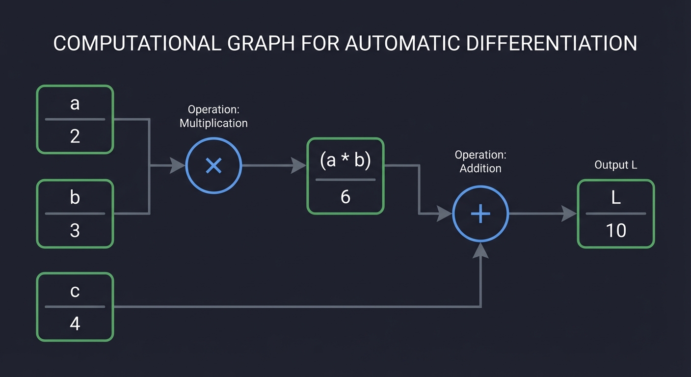
Forward Pass: Compute values from inputs to outputs (left to right) Backward Pass: Compute gradients from outputs to inputs (right to left)

3. Forward Mode vs Reverse Mode Automatic Differentiation

There are two ways to apply the chain rule automatically:

Forward Mode: Compute dx/da for all outputs x with respect to one input a

• Good when: many outputs, few inputs
• Compute: $\frac{\partial y_1}{\partial x}, \frac{\partial y_2}{\partial x}, \ldots$ in one pass

Reverse Mode: Compute dL/dx for one output L with respect to all inputs x

• Good when: one output (loss), many inputs (weights)
• Compute: $\frac{\partial L}{\partial x_1}, \frac{\partial L}{\partial x_2}, \ldots$ in one pass

Why ML Uses Reverse Mode: Neural networks have millions of parameters (inputs) and one scalar loss (output). Reverse mode computes all gradients in one backward pass. Forward mode would require one pass per parameter.

4. Python Magic Methods (add, mul, etc.)

Python’s operator overloading lets you define what +, *, -, /, ** mean for your objects:

class Value:
    def __init__(self, data):
        self.data = data

    def __add__(self, other):
        # Called when you write: a + b
        return Value(self.data + other.data)

    def __mul__(self, other):
        # Called when you write: a * b
        return Value(self.data * other.data)

    def __radd__(self, other):
        # Called when you write: 5 + a (other on left)
        return self + other

This is how we intercept math operations to build the graph.

5. Topological Sorting of DAGs

To compute gradients, we must process nodes in the correct order: children before parents (reverse topological order).

Forward order (topological):    a, b, c → (a*b) → ((a*b)+c) = L
Backward order (reverse topo):  L → (a*b)+c → (a*b) → a, b, c

Why this order for backward?
- We need dL/d(a*b) before we can compute dL/da and dL/db
- Gradients flow from the loss toward the inputs

Algorithm (Kahn’s or DFS-based):

1. Start at output node
2. Visit all children before visiting a node
3. Process in reverse of visit order

6. Gradient Accumulation

When a variable is used multiple times, its gradient is the SUM of all contributions:

Expression: L = a * a  (a is used twice!)

         ┌───────────┐
    a ───┤           ├──► [*] ──► L
         │   (same   │
    a ───┤    node)  │
         └───────────┘

dL/da = dL/d(first a) + dL/d(second a)
      = a + a = 2a

This is why we use:  self.grad += local_grad * upstream_grad
Not:                 self.grad = local_grad * upstream_grad

---

Deep Theoretical Foundation

A Brief History of Backpropagation

The chain rule is centuries old (Leibniz, 1676). But its application to neural networks has a fascinating history:

• 1960s: Control theory uses similar ideas (Pontryagin, Bryson, Dreyfus)
• 1970: Linnainmaa describes reverse mode AD for computer programs
• 1974: Werbos applies it to neural networks (PhD thesis, largely ignored)
• 1986: Rumelhart, Hinton, Williams publish “Learning representations by back-propagating errors” - This time, the world pays attention
• 2012: AlexNet uses GPUs to train deep networks with backprop. The deep learning revolution begins.

The key insight of the 1986 paper: we can train multi-layer networks by propagating error signals backward using the chain rule. Before this, people thought training deep networks was impossible.

The Mathematics of Reverse-Mode AD

Let’s formalize what we’re building. Consider a computational graph with:

• Input nodes: $x_1, x_2, \ldots, x_n$ (our parameters)
• Intermediate nodes: Results of operations
• Output node: $L$ (the loss)

Forward Pass: Compute each node’s value from its inputs, in topological order.

Backward Pass: For the output node: $\frac{\partial L}{\partial L} = 1$ (The output’s derivative with respect to itself)

For each node $v$ in reverse topological order: \(\frac{\partial L}{\partial v} = \sum_{u \in \text{children}(v)} \frac{\partial L}{\partial u} \cdot \frac{\partial u}{\partial v}\)

Where:

• $\frac{\partial L}{\partial u}$ is the gradient already computed for child $u$
• $\frac{\partial u}{\partial v}$ is the local derivative of the operation that created $u$

This is the key formula. The gradient of a node equals the sum over all children of (child’s gradient times local derivative).

Local Gradients for Common Operations

Each operation has a “local gradient” - the derivative of its output with respect to each input:

Operation	Output	$\frac{\partial \text{out}}{\partial a}$	$\frac{\partial \text{out}}{\partial b}$
a + b	$a + b$	$1$	$1$
a - b	$a - b$	$1$	$-1$
a * b	$a \cdot b$	$b$	$a$
a / b	$a / b$	$1/b$	$-a/b^2$
a ** n	$a^n$	$n \cdot a^{n-1}$	-
-a	$-a$	$-1$	-
exp(a)	$e^a$	$e^a$	-
log(a)	$\ln(a)$	$1/a$	-
tanh(a)	$\tanh(a)$	$1 - \tanh^2(a)$	-
relu(a)	$\max(0, a)$	$1$ if $a > 0$ else $0$	-

Why Reverse Mode is O(1) per Output

Forward mode AD computes $\frac{\partial L}{\partial x_i}$ for one $x_i$ at a time.

• To get all $n$ gradients: $O(n)$ forward passes
• Total work: $O(n \cdot \text{graph size})$

Reverse mode AD computes all $\frac{\partial L}{\partial x_i}$ in one backward pass.

• All $n$ gradients: $O(1)$ backward passes
• Total work: $O(\text{graph size})$

For a network with 100 million parameters, this is a 100-million-fold improvement!

Why This Is Called “Backpropagation”

“Backpropagation” = “Backward propagation of errors”

The gradient at each node represents “how much is this node responsible for the error?” This “error signal” propagates backward through the network.

Forward: inputs → predictions
Backward: error ← error signal flows backward ← loss

At each node:
  "How much should I blame myself for the final error?"
  = "How much did my children blame me?" (upstream gradient)
  × "How much did I contribute to my children?" (local gradient)

Comparison with Numerical Differentiation

You could compute gradients numerically: \(\frac{\partial L}{\partial x} \approx \frac{L(x + \epsilon) - L(x - \epsilon)}{2\epsilon}\)

Problems:

1. Requires $2n$ forward passes for $n$ parameters
2. Numerical precision issues (choose $\epsilon$ too small → floating point errors; too large → approximation errors)
3. Slow for large networks

When to Use: Numerical differentiation is excellent for testing. Compute gradients both ways and compare.

---

Real World Outcome

After building your autograd engine, you will be able to write code like this:

from my_engine import Value

# Create input values
x = Value(2.0)
y = Value(-3.0)
z = Value(10.0)

# Build a computational expression (this builds the graph!)
f = x * y + z  # f = 2.0 * (-3.0) + 10.0 = 4.0

# Compute all gradients with one call
f.backward()

# Access the gradients
print(f"Value of f: {f.data}")     # 4.0
print(f"x.grad: {x.grad}")         # -3.0 (Because df/dx = y = -3)
print(f"y.grad: {y.grad}")         # 2.0  (Because df/dy = x = 2)
print(f"z.grad: {z.grad}")         # 1.0  (Because df/dz = 1)

Expected Output:

Value of f: 4.0
x.grad: -3.0
y.grad: 2.0
z.grad: 1.0

And you can train actual neural networks:

from my_engine import Value, Neuron, Layer, MLP

# Create a simple MLP
model = MLP(3, [4, 4, 1])  # 3 inputs, two hidden layers of 4, 1 output

# Training data
xs = [
    [2.0, 3.0, -1.0],
    [3.0, -1.0, 0.5],
    [0.5, 1.0, 1.0],
    [1.0, 1.0, -1.0],
]
ys = [1.0, -1.0, -1.0, 1.0]  # targets

# Training loop
for epoch in range(100):
    # Forward pass
    predictions = [model(x) for x in xs]
    loss = sum((pred - target)**2 for pred, target in zip(predictions, ys))

    # Backward pass
    model.zero_grad()
    loss.backward()

    # Update weights
    for param in model.parameters():
        param.data -= 0.05 * param.grad

    if epoch % 10 == 0:
        print(f"Epoch {epoch}: Loss = {loss.data:.4f}")

# Test
print("\nPredictions after training:")
for x, y in zip(xs, ys):
    pred = model(x)
    print(f"Input: {x} Target: {y} Prediction: {pred.data:.4f}")

---

Solution Architecture

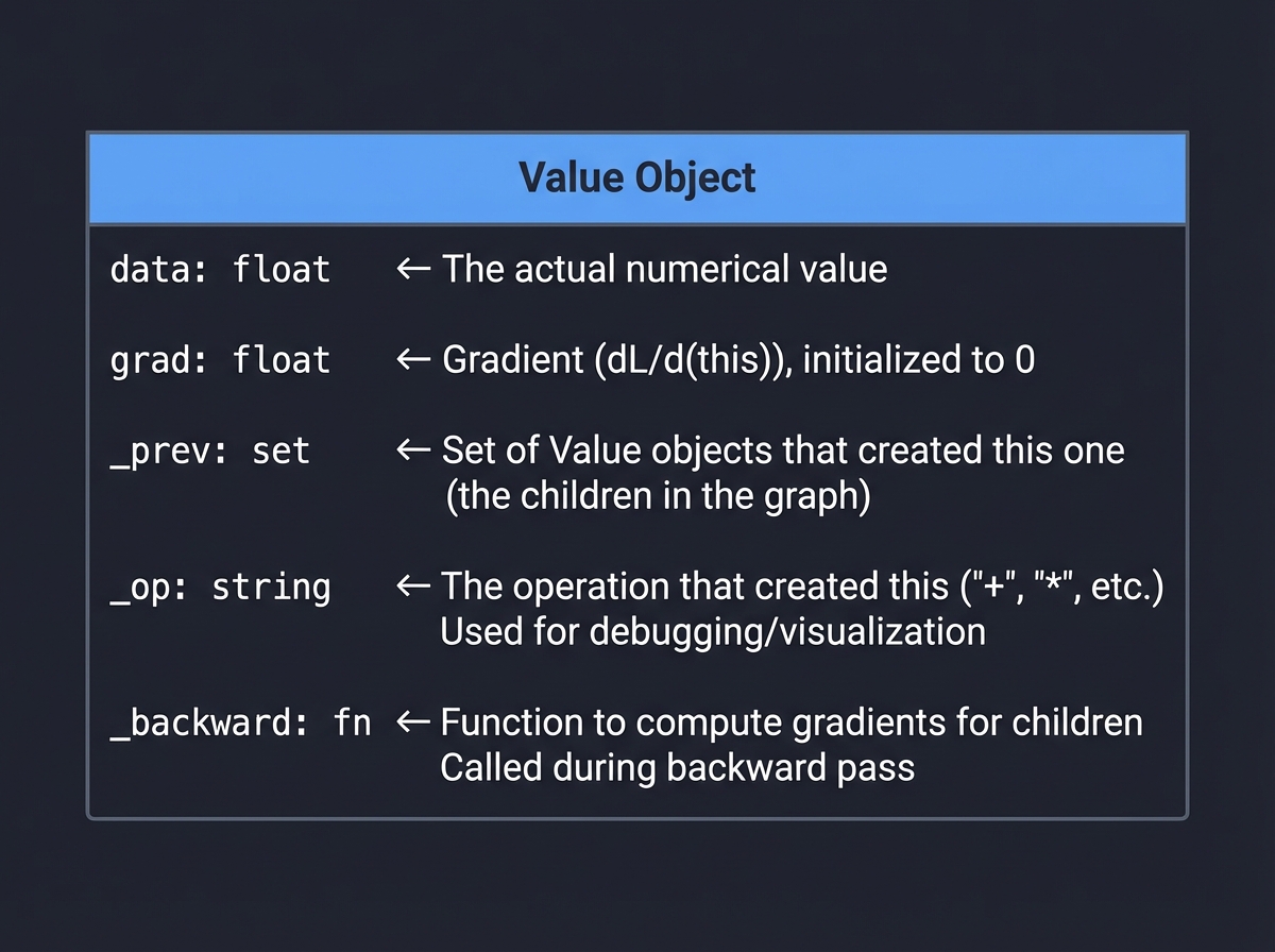
The Value Class Design

The Value class is the heart of your autograd engine. Each Value wraps a number and tracks:

┌────────────────────────────────────────────────────────────────────────────┐
│                              Value Object                                   │
├────────────────────────────────────────────────────────────────────────────┤
│                                                                             │
│  ┌─────────────────┐                                                        │
│  │  data: float    │ ← The actual numerical value                           │
│  ├─────────────────┤                                                        │
│  │  grad: float    │ ← Gradient (dL/d(this)), initialized to 0             │
│  ├─────────────────┤                                                        │
│  │  _prev: set     │ ← Set of Value objects that created this one          │
│  ├─────────────────┤    (the children in the graph)                         │
│  │  _op: string    │ ← The operation that created this ('+', '*', etc.)    │
│  ├─────────────────┤    Used for debugging/visualization                    │
│  │  _backward: fn  │ ← Function to compute gradients for children           │
│  └─────────────────┘    Called during backward pass                         │
│                                                                             │
└────────────────────────────────────────────────────────────────────────────┘

The Computational Graph

When you write f = x * y + z, this builds:

EXPRESSION: f = (x * y) + z
─────────────────────────────────────────────────────────────────────────────

                    ┌─────────────┐
   x ──────────────►│             │
   (data=2.0)       │     *       │──────► (x*y) ─────────┐
   (grad=?)         │             │        (data=-6.0)    │
                    └─────────────┘        (grad=?)       │    ┌─────────────┐
                           ▲                               │    │             │
                           │                               ├───►│     +       │──► f
   y ──────────────────────┘                               │    │             │   (data=4.0)
   (data=-3.0)                                             │    └─────────────┘   (grad=1.0)
   (grad=?)                                                │           ▲
                                                           │           │
   z ──────────────────────────────────────────────────────┘───────────┘
   (data=10.0)
   (grad=?)

FORWARD PASS (left to right):
  1. x*y = 2.0 * (-3.0) = -6.0
  2. (x*y)+z = -6.0 + 10.0 = 4.0

BACKWARD PASS (right to left):
  1. f.grad = 1.0 (output gradient is always 1)
  2. (x*y).grad = f.grad * d(f)/d(x*y) = 1.0 * 1 = 1.0
     z.grad = f.grad * d(f)/dz = 1.0 * 1 = 1.0
  3. x.grad = (x*y).grad * d(x*y)/dx = 1.0 * y = 1.0 * (-3.0) = -3.0
     y.grad = (x*y).grad * d(x*y)/dy = 1.0 * x = 1.0 * 2.0 = 2.0

The Backward Function Pattern

Each operation stores a _backward function that knows how to propagate gradients:

def __mul__(self, other):
    out = Value(self.data * other.data, (self, other), '*')

    def _backward():
        # d(self * other)/d(self) = other
        # d(self * other)/d(other) = self
        self.grad += other.data * out.grad
        other.grad += self.data * out.grad

    out._backward = _backward
    return out

Critical Pattern:

• out.grad is the upstream gradient (gradient of loss w.r.t. this node)
• other.data and self.data are local gradients
• We accumulate (+=) because a node might be used multiple times

Topological Sort for Backward Order

The backward pass must visit nodes in reverse topological order:

TOPOLOGICAL SORT ALGORITHM (using DFS):
─────────────────────────────────────────────────────────────────────────────

def build_topo(v, visited, topo):
    if v not in visited:
        visited.add(v)
        for child in v._prev:      # Visit all children first
            build_topo(child, visited, topo)
        topo.append(v)             # Then add self
    return topo

# For f = (x*y) + z:
topo = build_topo(f, set(), [])
# topo = [x, y, (x*y), z, f]

# Backward processes in REVERSE:
for v in reversed(topo):           # [f, z, (x*y), y, x]
    v._backward()


VISUALIZATION OF BACKWARD ORDER:
─────────────────────────────────────────────────────────────────────────────

    Order:   1st      2nd       3rd      4th      5th
             ▼        ▼         ▼        ▼        ▼
           ┌───┐    ┌───┐    ┌─────┐  ┌───┐    ┌───┐
           │ f │ ←─ │ z │    │ x*y │  │ y │    │ x │
           └───┘    └───┘    └─────┘  └───┘    └───┘
             │                   │        │        │
        grad=1.0            grad=1.0  grad=2.0  grad=-3.0
        (start)             (from +)  (from *) (from *)

---

Phased Implementation Guide

Phase 1: The Value Class Foundation (Day 1)

Goal: Create a Value class that stores data and gradient

class Value:
    def __init__(self, data, _children=(), _op=''):
        self.data = data
        self.grad = 0.0
        self._prev = set(_children)
        self._op = _op
        self._backward = lambda: None

    def __repr__(self):
        return f"Value(data={self.data}, grad={self.grad})"

Test:

x = Value(5.0)
print(x)  # Value(data=5.0, grad=0.0)

Checkpoint: You can create Value objects and they store data and grad.

Phase 2: Addition with Graph Building (Day 2)

Goal: Implement __add__ that builds the graph and backward function

def __add__(self, other):
    other = other if isinstance(other, Value) else Value(other)
    out = Value(self.data + other.data, (self, other), '+')

    def _backward():
        self.grad += 1.0 * out.grad   # d(a+b)/da = 1
        other.grad += 1.0 * out.grad  # d(a+b)/db = 1

    out._backward = _backward
    return out

def __radd__(self, other):  # Handles: 5 + Value
    return self + other

Explanation of the backward function:

For addition: out = a + b
  - d(out)/d(a) = 1    (local gradient for a)
  - d(out)/d(b) = 1    (local gradient for b)

Chain rule:
  - d(L)/d(a) = d(L)/d(out) * d(out)/d(a) = out.grad * 1
  - d(L)/d(b) = d(L)/d(out) * d(out)/d(b) = out.grad * 1

Test:

a = Value(2.0)
b = Value(3.0)
c = a + b
print(c)  # Value(data=5.0, grad=0.0)
print(c._prev)  # {a, b}

Phase 3: Multiplication, Subtraction, Power (Days 3-4)

Goal: Implement remaining arithmetic operations

def __mul__(self, other):
    other = other if isinstance(other, Value) else Value(other)
    out = Value(self.data * other.data, (self, other), '*')

    def _backward():
        self.grad += other.data * out.grad  # d(a*b)/da = b
        other.grad += self.data * out.grad  # d(a*b)/db = a

    out._backward = _backward
    return out

def __rmul__(self, other):
    return self * other

def __neg__(self):
    return self * -1

def __sub__(self, other):
    return self + (-other)

def __rsub__(self, other):
    return other + (-self)

def __pow__(self, n):
    assert isinstance(n, (int, float)), "only supporting int/float powers"
    out = Value(self.data ** n, (self,), f'**{n}')

    def _backward():
        # d(x^n)/dx = n * x^(n-1)
        self.grad += n * (self.data ** (n - 1)) * out.grad

    out._backward = _backward
    return out

def __truediv__(self, other):
    return self * (other ** -1)

def __rtruediv__(self, other):
    return other * (self ** -1)

Visualization of multiplication backward:

MULTIPLICATION: out = a * b
─────────────────────────────────────────────────────────────────────────────

Forward:
    a ─────┐
    (2.0)  │
           ├──► [*] ──► out
    b ─────┘          (6.0)
    (3.0)

Backward:
    a.grad += b.data * out.grad
           += 3.0 * 1.0
           += 3.0

    b.grad += a.data * out.grad
           += 2.0 * 1.0
           += 2.0

Why?
  - If you wiggle 'a' by 1, 'out' wiggles by b = 3
  - If you wiggle 'b' by 1, 'out' wiggles by a = 2

Test:

a = Value(2.0)
b = Value(3.0)
c = a * b
d = a ** 2
print(c.data)  # 6.0
print(d.data)  # 4.0

Phase 4: The Backward Pass Infrastructure (Day 5)

Goal: Implement topological sort and the backward() method

def backward(self):
    # Build topological order
    topo = []
    visited = set()

    def build_topo(v):
        if v not in visited:
            visited.add(v)
            for child in v._prev:
                build_topo(child)
            topo.append(v)

    build_topo(self)

    # Initialize output gradient to 1
    self.grad = 1.0

    # Apply chain rule in reverse order
    for node in reversed(topo):
        node._backward()

Trace through example:

Expression: f = (x * y) + z where x=2, y=-3, z=10

Step 1: Build topological order
  build_topo(f)
    build_topo(x*y)
      build_topo(x)         → topo = [x]
      build_topo(y)         → topo = [x, y]
      append(x*y)           → topo = [x, y, x*y]
    build_topo(z)           → topo = [x, y, x*y, z]
    append(f)               → topo = [x, y, x*y, z, f]

Step 2: Process in reverse: [f, z, x*y, y, x]
  f.grad = 1.0              (initialize)
  f._backward()             → (x*y).grad += 1.0, z.grad += 1.0
  z._backward()             → (nothing, z is a leaf)
  (x*y)._backward()         → x.grad += y.data * 1.0 = -3.0
                            → y.grad += x.data * 1.0 = 2.0
  y._backward()             → (nothing, y is a leaf)
  x._backward()             → (nothing, x is a leaf)

Result:
  x.grad = -3.0
  y.grad = 2.0
  z.grad = 1.0

Test:

x = Value(2.0)
y = Value(-3.0)
z = Value(10.0)
f = x * y + z

f.backward()

assert x.grad == -3.0
assert y.grad == 2.0
assert z.grad == 1.0
print("Phase 4 tests passed!")

Phase 5: Handling Repeated Variables (Day 6)

Goal: Ensure gradient accumulation works for variables used multiple times

# Test case: L = a * a (same variable used twice)
a = Value(3.0)
L = a * a

L.backward()
print(a.grad)  # Should be 6.0 (dL/da = 2a = 2*3 = 6)

The issue: If a is used twice, both usages contribute to the gradient.

Visualization:

REPEATED VARIABLE: L = a * a
─────────────────────────────────────────────────────────────────────────────

The computational graph:

          ┌─────────────────┐
    a ────┤   same node     ├────► [*] ────► L
    (3.0) │   referenced    │      (9.0)
          │   twice!        │
          └─────────────────┘

This is NOT two separate nodes. The single 'a' node has two edges leading to '*'.

During backward:
  _backward() for multiplication is called once
  BUT it adds to a.grad TWICE (once for each input position):

    a.grad += other.data * out.grad   # other IS a here! = 3.0 * 1.0
    other.grad += self.data * out.grad # self IS a here! = 3.0 * 1.0

  Both lines update a.grad because self == other == a
  Final: a.grad = 3.0 + 3.0 = 6.0 ✓

This is why we use += and not = for gradients!

Test:

# Test 1: a * a
a = Value(3.0)
L = a * a
L.backward()
assert a.grad == 6.0, f"Expected 6.0, got {a.grad}"

# Test 2: a + a
a = Value(3.0)
L = a + a
L.backward()
assert a.grad == 2.0, f"Expected 2.0, got {a.grad}"

# Test 3: a * a + a
a = Value(3.0)
L = a * a + a  # dL/da = 2a + 1 = 7
L.backward()
assert a.grad == 7.0, f"Expected 7.0, got {a.grad}"

print("Phase 5 tests passed!")

Phase 6: Activation Functions (Day 7)

Goal: Implement tanh and relu activation functions

import math

def tanh(self):
    x = self.data
    t = (math.exp(2*x) - 1) / (math.exp(2*x) + 1)
    out = Value(t, (self,), 'tanh')

    def _backward():
        # d(tanh(x))/dx = 1 - tanh^2(x)
        self.grad += (1 - t**2) * out.grad

    out._backward = _backward
    return out

def relu(self):
    out = Value(max(0, self.data), (self,), 'ReLU')

    def _backward():
        # d(relu(x))/dx = 1 if x > 0 else 0
        self.grad += (1.0 if self.data > 0 else 0.0) * out.grad

    out._backward = _backward
    return out

def exp(self):
    x = self.data
    out = Value(math.exp(x), (self,), 'exp')

    def _backward():
        # d(e^x)/dx = e^x
        self.grad += out.data * out.grad

    out._backward = _backward
    return out

Visualization of tanh backward:

TANH ACTIVATION:
─────────────────────────────────────────────────────────────────────────────

               tanh function               derivative of tanh
                   ▲ y                          ▲ dy/dx
               1.0 ├────────────────         1.0├───┐
                   │        ═══════              │   │
                   │      ╱                      │   │
                   │    ╱                        │   └───┐
               0.0 ├──╱────────────          0.5├       └───┐
                   │╱                            │           └───────
                   │                         0.0├───────────────────
              -1.0 ├═══════                     └───┬───┬───┬───► x
                   └───────────► x               -3  -1   1   3

tanh squashes values to [-1, 1]
Derivative is highest at x=0 (=1), lowest at extremes (→0)

In code:
  forward:  out.data = tanh(self.data)
  backward: self.grad += (1 - out.data**2) * out.grad

Test:

x = Value(0.5)
y = x.tanh()
y.backward()
print(f"tanh(0.5) = {y.data:.4f}")  # ~0.4621
print(f"d(tanh)/dx at 0.5 = {x.grad:.4f}")  # ~0.7864

# Verify with numerical gradient
eps = 1e-5
numerical = (math.tanh(0.5 + eps) - math.tanh(0.5 - eps)) / (2 * eps)
print(f"Numerical gradient: {numerical:.4f}")

Phase 7: Building a Neural Network (Days 8-10)

Goal: Create Neuron, Layer, and MLP classes using your Value objects

import random

class Neuron:
    def __init__(self, num_inputs):
        self.w = [Value(random.uniform(-1, 1)) for _ in range(num_inputs)]
        self.b = Value(random.uniform(-1, 1))

    def __call__(self, x):
        # w * x + b
        act = sum((wi * xi for wi, xi in zip(self.w, x)), self.b)
        return act.tanh()

    def parameters(self):
        return self.w + [self.b]


class Layer:
    def __init__(self, num_inputs, num_outputs):
        self.neurons = [Neuron(num_inputs) for _ in range(num_outputs)]

    def __call__(self, x):
        outs = [n(x) for n in self.neurons]
        return outs[0] if len(outs) == 1 else outs

    def parameters(self):
        return [p for neuron in self.neurons for p in neuron.parameters()]


class MLP:
    def __init__(self, num_inputs, layer_sizes):
        sizes = [num_inputs] + layer_sizes
        self.layers = [Layer(sizes[i], sizes[i+1]) for i in range(len(layer_sizes))]

    def __call__(self, x):
        for layer in self.layers:
            x = layer(x)
        return x

    def parameters(self):
        return [p for layer in self.layers for p in layer.parameters()]

    def zero_grad(self):
        for p in self.parameters():
            p.grad = 0.0

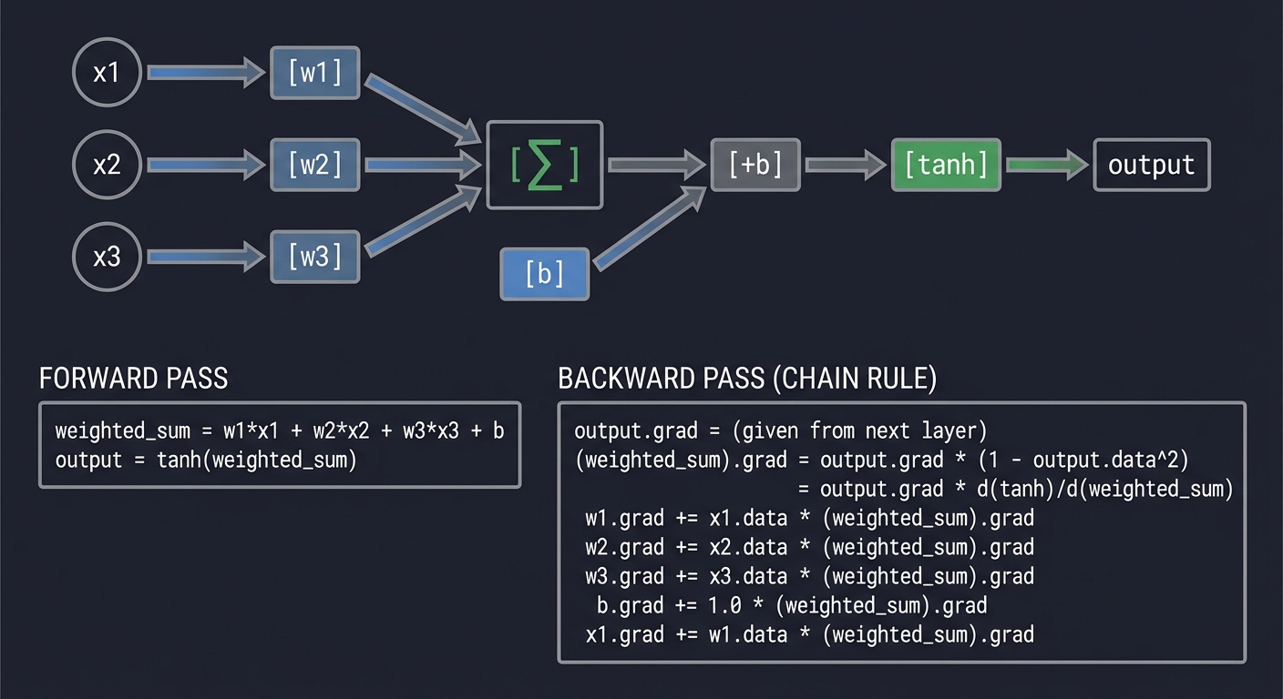
Visualization of a Neuron:

NEURON: out = tanh(w1*x1 + w2*x2 + w3*x3 + b)
─────────────────────────────────────────────────────────────────────────────

  x1 ──►[w1]──┐
              │
  x2 ──►[w2]──┼──►[Σ]──►[+b]──►[tanh]──► output
              │
  x3 ──►[w3]──┘

Forward:
  weighted_sum = w1*x1 + w2*x2 + w3*x3 + b
  output = tanh(weighted_sum)

Backward (chain rule flows back):
  output.grad = (given from next layer)

  (weighted_sum).grad = output.grad * (1 - output.data^2)
                      = output.grad * d(tanh)/d(weighted_sum)

  w1.grad += x1.data * (weighted_sum).grad
  w2.grad += x2.data * (weighted_sum).grad
  w3.grad += x3.data * (weighted_sum).grad
  b.grad += 1.0 * (weighted_sum).grad

  x1.grad += w1.data * (weighted_sum).grad
  (etc.)

Test:

# Create a small network
model = MLP(3, [4, 4, 1])
print(f"Number of parameters: {len(model.parameters())}")

# Forward pass
x = [Value(1.0), Value(2.0), Value(-1.0)]
output = model(x)
print(f"Output: {output.data:.4f}")

# Backward pass
output.backward()
print(f"First weight gradient: {model.parameters()[0].grad:.4f}")

Phase 8: Training Loop (Days 11-14)

Goal: Train your MLP on a simple dataset

# Binary classification dataset
xs = [
    [2.0, 3.0, -1.0],
    [3.0, -1.0, 0.5],
    [0.5, 1.0, 1.0],
    [1.0, 1.0, -1.0],
]
ys = [1.0, -1.0, -1.0, 1.0]

# Create model
model = MLP(3, [4, 4, 1])
print(f"Training with {len(model.parameters())} parameters")

# Training hyperparameters
learning_rate = 0.1
epochs = 100

for epoch in range(epochs):
    # Forward pass: compute predictions
    predictions = [model(x) for x in xs]

    # Compute loss (mean squared error)
    loss = sum((pred - target)**2 for pred, target in zip(predictions, ys))

    # Zero gradients (IMPORTANT: must do before backward!)
    model.zero_grad()

    # Backward pass: compute gradients
    loss.backward()

    # Update weights (gradient descent)
    for p in model.parameters():
        p.data -= learning_rate * p.grad

    if epoch % 10 == 0:
        print(f"Epoch {epoch:3d}: Loss = {loss.data:.4f}")

# Final predictions
print("\nFinal predictions:")
for x, y in zip(xs, ys):
    pred = model(x)
    print(f"  Input: {x}, Target: {y:+.1f}, Prediction: {pred.data:+.4f}")

Expected Output:

Training with 41 parameters
Epoch   0: Loss = 4.3127
Epoch  10: Loss = 0.8234
Epoch  20: Loss = 0.1245
Epoch  30: Loss = 0.0312
Epoch  40: Loss = 0.0089
Epoch  50: Loss = 0.0034
...

Final predictions:
  Input: [2.0, 3.0, -1.0], Target: +1.0, Prediction: +0.9823
  Input: [3.0, -1.0, 0.5], Target: -1.0, Prediction: -0.9756
  Input: [0.5, 1.0, 1.0], Target: -1.0, Prediction: -0.9812
  Input: [1.0, 1.0, -1.0], Target: +1.0, Prediction: +0.9734

---

Questions to Guide Your Design

Before writing code, think through these design decisions:

Value Class Design

• How will you handle operations with Python scalars? e.g., Value(3) + 5
  • Answer: Check if other is a Value; if not, wrap it in Value(other)
• Should _backward be None or a no-op lambda by default?
  • Answer: A no-op lambda: None simplifies the backward loop
• How do you prevent backward() from being called twice?
  • Consider: Karpathy’s micrograd allows this, but PyTorch raises an error

Gradient Management

• When should gradients be zeroed?
  • Answer: Before each backward pass, call model.zero_grad()
• What happens if you call backward() twice?
  • Answer: Gradients accumulate. Sometimes desired (RNNs), sometimes not.
• Should leaf nodes have _backward functions?
  • Answer: Yes, but they do nothing (no-op)

Numerical Stability

• What happens with exp(1000)?
  • Problem: Overflow! Consider clamping or using stable implementations
• What about division by zero in power?
  • Example: Value(0) ** -1 = division by zero

---

Thinking Exercise: Trace the Backward Pass by Hand

Before implementing, trace this example completely by hand:

Expression: L = ((a * b) + c) * (a + d)

Values: a=2, b=3, c=4, d=5

Step 1: Draw the computational graph

YOUR TASK: Complete this diagram
─────────────────────────────────────────────────────────────────────────────

     a ──────┬─────────────────────────────────────┐
     (2)     │                                     │
             ▼                                     ▼
     b ──► [ * ] ──► t1 ──┐                     [   ] ──► t3 ──┐
     (3)            (?)    │                    (?)      (?)    │
                           ▼                                    ▼
     c ─────────────► [ + ] ──► t2 ────────────────────────► [ * ] ──► L
     (4)                   (?)                                    (?)

     d ────────────────────────────────────────────────────────┘
     (5)

Fill in:
  t1 = a * b = ?
  t2 = t1 + c = ?
  t3 = a + d = ?
  L = t2 * t3 = ?

Step 2: Compute forward pass values

t1 = a * b = 2 * 3 = 6
t2 = t1 + c = 6 + 4 = 10
t3 = a + d = 2 + 5 = 7
L = t2 * t3 = 10 * 7 = 70

Step 3: Compute backward pass (fill in the gradients)

YOUR TASK: Complete the gradient computation
─────────────────────────────────────────────────────────────────────────────

L.grad = 1.0 (start)

For L = t2 * t3:
  t2.grad += t3.data * L.grad = ? * 1.0 = ?
  t3.grad += t2.data * L.grad = ? * 1.0 = ?

For t2 = t1 + c:
  t1.grad += 1.0 * t2.grad = 1.0 * ? = ?
  c.grad += 1.0 * t2.grad = 1.0 * ? = ?

For t3 = a + d:
  (contribution to a.grad) += 1.0 * t3.grad = 1.0 * ? = ?
  d.grad += 1.0 * t3.grad = 1.0 * ? = ?

For t1 = a * b:
  (contribution to a.grad) += b.data * t1.grad = ? * ? = ?
  b.grad += a.data * t1.grad = ? * ? = ?

FINAL GRADIENTS (remember a is used twice!):
  a.grad = (from t1) + (from t3) = ? + ? = ?
  b.grad = ?
  c.grad = ?
  d.grad = ?

Solution:

L.grad = 1.0

For L = t2 * t3:
  t2.grad = 7 * 1.0 = 7
  t3.grad = 10 * 1.0 = 10

For t2 = t1 + c:
  t1.grad = 1.0 * 7 = 7
  c.grad = 1.0 * 7 = 7

For t3 = a + d:
  a.grad += 1.0 * 10 = 10
  d.grad = 1.0 * 10 = 10

For t1 = a * b:
  a.grad += 3 * 7 = 21
  b.grad = 2 * 7 = 14

FINAL:
  a.grad = 10 + 21 = 31  (used in both t1 and t3!)
  b.grad = 14
  c.grad = 7
  d.grad = 10

Verify: Compute dL/da numerically

def f(a, b, c, d):
    return ((a * b) + c) * (a + d)

a, b, c, d = 2, 3, 4, 5
eps = 1e-5
numerical_grad = (f(a+eps, b, c, d) - f(a-eps, b, c, d)) / (2*eps)
# numerical_grad ≈ 31.0 ✓

---

Testing Strategy

1. Unit Tests for Each Operation

Test each operation’s forward and backward independently:

def test_add():
    a = Value(2.0)
    b = Value(3.0)
    c = a + b
    c.backward()
    assert c.data == 5.0
    assert a.grad == 1.0
    assert b.grad == 1.0

def test_mul():
    a = Value(2.0)
    b = Value(3.0)
    c = a * b
    c.backward()
    assert c.data == 6.0
    assert a.grad == 3.0  # d(a*b)/da = b
    assert b.grad == 2.0  # d(a*b)/db = a

def test_pow():
    a = Value(3.0)
    b = a ** 2
    b.backward()
    assert b.data == 9.0
    assert a.grad == 6.0  # d(x^2)/dx = 2x = 6

2. Numerical Gradient Verification

Compare your gradients with numerical approximations:

def numerical_gradient(f, x, eps=1e-5):
    """Compute gradient numerically using central difference"""
    original = x.data

    x.data = original + eps
    f_plus = f().data

    x.data = original - eps
    f_minus = f().data

    x.data = original  # restore
    return (f_plus - f_minus) / (2 * eps)

def test_numerical_vs_autograd():
    a = Value(2.0)
    b = Value(3.0)

    def loss_fn():
        return (a * b + a**2).tanh()

    # Autograd gradient
    loss = loss_fn()
    loss.backward()
    autograd_grad_a = a.grad

    # Numerical gradient
    a.grad = 0  # reset
    numerical_grad_a = numerical_gradient(loss_fn, a)

    assert abs(autograd_grad_a - numerical_grad_a) < 1e-4, \
        f"Mismatch: autograd={autograd_grad_a}, numerical={numerical_grad_a}"

3. Comparison with PyTorch

The gold standard - compare with PyTorch:

import torch

def test_against_pytorch():
    # Create values in both systems
    x_mine = Value(2.0)
    y_mine = Value(3.0)
    z_mine = x_mine * y_mine + x_mine**2
    z_mine.backward()

    x_torch = torch.tensor(2.0, requires_grad=True)
    y_torch = torch.tensor(3.0, requires_grad=True)
    z_torch = x_torch * y_torch + x_torch**2
    z_torch.backward()

    # Compare
    assert abs(z_mine.data - z_torch.item()) < 1e-6
    assert abs(x_mine.grad - x_torch.grad.item()) < 1e-6
    assert abs(y_mine.grad - y_torch.grad.item()) < 1e-6

    print("Matches PyTorch! ✓")

4. Complex Expression Tests

Test complicated expressions that exercise multiple paths:

def test_complex_expression():
    a = Value(2.0)
    b = Value(3.0)
    c = Value(-1.0)

    # Complex expression with repeated variables
    d = a * b
    e = d + c
    f = e * a  # a is used again!
    g = f.tanh()

    g.backward()

    # Verify with numerical gradients
    def compute(a_val, b_val, c_val):
        import math
        d = a_val * b_val
        e = d + c_val
        f = e * a_val
        return math.tanh(f)

    eps = 1e-5
    numerical_a = (compute(2.0+eps, 3.0, -1.0) - compute(2.0-eps, 3.0, -1.0)) / (2*eps)

    assert abs(a.grad - numerical_a) < 1e-4

---

Common Pitfalls and Debugging Tips

Pitfall 1: Forgetting to Zero Gradients

Problem:

for epoch in range(100):
    loss = model(x)
    loss.backward()  # Gradients ACCUMULATE!
    # ... update weights

Gradients keep growing because they accumulate across epochs.

Solution:

for epoch in range(100):
    model.zero_grad()  # Clear gradients before backward
    loss = model(x)
    loss.backward()
    # ... update weights

Pitfall 2: Using = Instead of += in Backward

Problem:

def _backward():
    self.grad = other.data * out.grad  # WRONG!

If a variable is used twice, the second assignment overwrites the first.

Solution:

def _backward():
    self.grad += other.data * out.grad  # Correct: accumulate

Pitfall 3: Not Handling Python Scalars

Problem:

a = Value(5)
b = a + 3  # TypeError: unsupported operand types

Solution:

def __add__(self, other):
    other = other if isinstance(other, Value) else Value(other)
    # ...

def __radd__(self, other):  # For: 3 + a
    return self + other

Pitfall 4: Wrong Topological Order

Problem: Processing nodes in wrong order gives wrong gradients.

Symptom: Gradients are zero or NaN for some variables.

Debugging:

def backward(self):
    topo = []
    visited = set()

    def build_topo(v):
        if v not in visited:
            visited.add(v)
            for child in v._prev:
                build_topo(child)
            topo.append(v)
            print(f"Added to topo: {v._op or 'leaf'} = {v.data}")  # DEBUG

    build_topo(self)
    print(f"Topo order: {[n._op or 'leaf' for n in topo]}")  # DEBUG
    # ...

Pitfall 5: Numerical Instability

Problem: Operations like exp(100) or log(0) cause overflow/underflow.

Solutions:

def exp(self):
    # Clamp to prevent overflow
    x = max(min(self.data, 88), -88)  # exp(88) ≈ 1.6e38, close to float max
    out = Value(math.exp(x), (self,), 'exp')
    # ...

def log(self):
    # Prevent log(0)
    x = max(self.data, 1e-8)
    out = Value(math.log(x), (self,), 'log')
    # ...

Debugging Checklist

When gradients are wrong:

1. Print the computational graph:

   def trace_graph(root, indent=0):
    print(" " * indent + f"{root._op or 'leaf'}: data={root.data:.4f}, grad={root.grad:.4f}")
    for child in root._prev:
        trace_graph(child, indent + 2)
   

2. Verify individual operations:

   # Isolate the operation
   a = Value(2.0)
   b = Value(3.0)
   c = a * b
   c.backward()
   print(f"Expected: a.grad=3.0, b.grad=2.0")
   print(f"Got: a.grad={a.grad}, b.grad={b.grad}")
   

3. Compare with numerical gradient:

   eps = 1e-5
   a = Value(2.0)
   def f(val):
    a.data = val
    result = (a * Value(3.0)).data
    a.data = 2.0  # restore
    return result
   numerical = (f(2.0 + eps) - f(2.0 - eps)) / (2 * eps)
   print(f"Numerical: {numerical}")
   

---

Interview Questions

If you build an autograd engine, expect these questions in ML interviews:

Understanding Questions

1. “Explain automatic differentiation. How is it different from symbolic or numerical differentiation?”

   • Symbolic: Manipulates formulas (like Wolfram Alpha). d/dx(x^2) = 2x. Exact but can create expression explosion.
   • Numerical: Finite differences. (f(x+h) - f(x-h)) / 2h. Simple but slow and numerically unstable.
   • Automatic: Tracks operations during execution and applies chain rule. Exact and efficient.

2. “Why do we use reverse-mode AD instead of forward-mode for neural networks?”

   • Neural nets have millions of inputs (weights) and one output (loss).
   • Reverse mode computes all gradients in one pass (O(1) w.r.t. number of inputs).
   • Forward mode requires one pass per input (O(n) passes for n inputs).

3. “What is the computational graph and why does PyTorch build it dynamically?”

   • Graph is a DAG where nodes are values and edges are operations.
   • Dynamic (define-by-run): Graph is built as code executes.
   • Allows control flow (if/else, loops) to affect graph structure.
   • TensorFlow v1 was static; TensorFlow v2 and PyTorch are dynamic.

Implementation Questions

1. “Why do we accumulate gradients with += instead of =?”

   • A variable might be used multiple times in an expression.
   • Each usage contributes to the total gradient.
   • L = x * x means dL/dx = x + x = 2x (two contributions).

2. “What happens when you call backward() twice?”

   • Gradients accumulate, giving wrong results.
   • PyTorch raises: “Trying to backward through the graph a second time”
   • Solution: retain_graph=True or recompute forward pass.

3. “How do you handle non-differentiable operations like ReLU at x=0?”

   • ReLU’s derivative is undefined at exactly 0.
   • We define it as 0 (subgradient) by convention.
   • In practice, hitting exactly 0 is rare.

Design Questions

1. “How would you add GPU support?”

   • Store data as GPU tensors (cupy, PyTorch CUDA tensors).
   • Operations become kernel launches.
   • Graph structure stays the same.

2. “How would you implement checkpointing to save memory?”

   • Don’t store intermediate activations.
   • Recompute during backward pass.
   • Trade computation for memory.

---

Hints in Layers

Stuck? Read only the hint level you need:

Challenge: Backward function captures wrong values

Hint Level 1 (Conceptual): The _backward function needs to reference values that exist when it’s called, not when it’s defined.

Hint Level 2 (Direction): Python closures capture variables by reference, not by value. This can cause issues if variables change.

Hint Level 3 (Specific): In the _backward function, use self.data and other.data, not captured local variables that might change.

Hint Level 4 (Code):

# WRONG - 'other' might change before _backward is called
def __add__(self, other):
    out = Value(self.data + other.data, (self, other), '+')
    captured_other = other  # This might not be what you expect!

# CORRECT - reference actual objects that won't change
def __add__(self, other):
    other = other if isinstance(other, Value) else Value(other)
    out = Value(self.data + other.data, (self, other), '+')

    def _backward():
        self.grad += out.grad   # self and other are the actual Value objects
        other.grad += out.grad  # They're in _prev, so they're stable
    out._backward = _backward
    return out

Challenge: Topological sort isn’t working

Hint Level 1 (Conceptual): The order matters. You need to process children before parents in the backward pass.

Hint Level 2 (Direction): Use DFS. Mark nodes as visited, process children first, then append self to list.

Hint Level 3 (Specific): The tricky part is handling the output node. Initialize output.grad = 1.0 AFTER building topo but BEFORE iterating.

Hint Level 4 (Code):

def backward(self):
    topo = []
    visited = set()

    def build_topo(v):
        if v not in visited:
            visited.add(v)
            for child in v._prev:
                build_topo(child)
            topo.append(v)

    build_topo(self)

    # IMPORTANT: Set gradient of output to 1.0
    self.grad = 1.0

    # Process in reverse (output first)
    for v in reversed(topo):
        v._backward()

Challenge: Training loss isn’t decreasing

Hint Level 1 (Conceptual): If loss isn’t decreasing, gradients might be wrong or updates might be wrong.

Hint Level 2 (Direction): Print gradients after backward. Are they reasonable? Non-zero? Not NaN?

Hint Level 3 (Specific): Common issues:

• Not calling zero_grad() before backward
• Learning rate too high (loss oscillates) or too low (loss barely moves)
• Wrong sign in update (should be -= learning_rate * grad, not +=)

Hint Level 4 (Code):

for epoch in range(100):
    # 1. Zero gradients
    model.zero_grad()

    # 2. Forward
    pred = model(x)
    loss = (pred - y) ** 2

    # 3. Backward
    loss.backward()

    # 4. Debug - print some gradients
    if epoch == 0:
        for i, p in enumerate(model.parameters()[:3]):
            print(f"Param {i}: grad = {p.grad}")

    # 5. Update (minus sign!)
    for p in model.parameters():
        p.data -= 0.1 * p.grad

---

Extensions and Challenges

Extension 1: Add More Operations

Implement these additional operations:

def log(self):
    """Natural logarithm"""
    out = Value(math.log(self.data), (self,), 'log')
    def _backward():
        self.grad += (1.0 / self.data) * out.grad  # d(log x)/dx = 1/x
    out._backward = _backward
    return out

def sin(self):
    """Sine function"""
    out = Value(math.sin(self.data), (self,), 'sin')
    def _backward():
        self.grad += math.cos(self.data) * out.grad  # d(sin x)/dx = cos x
    out._backward = _backward
    return out

def sigmoid(self):
    """Sigmoid activation"""
    s = 1 / (1 + math.exp(-self.data))
    out = Value(s, (self,), 'sigmoid')
    def _backward():
        self.grad += (s * (1 - s)) * out.grad  # d(sigmoid)/dx = sigmoid * (1-sigmoid)
    out._backward = _backward
    return out

Extension 2: Implement an Optimizer

Create an SGD optimizer class:

class SGD:
    def __init__(self, parameters, lr=0.01):
        self.parameters = parameters
        self.lr = lr

    def step(self):
        for p in self.parameters:
            p.data -= self.lr * p.grad

    def zero_grad(self):
        for p in self.parameters:
            p.grad = 0.0


class Adam:
    def __init__(self, parameters, lr=0.001, beta1=0.9, beta2=0.999, eps=1e-8):
        self.parameters = parameters
        self.lr = lr
        self.beta1 = beta1
        self.beta2 = beta2
        self.eps = eps
        self.t = 0
        self.m = [0.0 for _ in parameters]  # First moment
        self.v = [0.0 for _ in parameters]  # Second moment

    def step(self):
        self.t += 1
        for i, p in enumerate(self.parameters):
            self.m[i] = self.beta1 * self.m[i] + (1 - self.beta1) * p.grad
            self.v[i] = self.beta2 * self.v[i] + (1 - self.beta2) * (p.grad ** 2)

            m_hat = self.m[i] / (1 - self.beta1 ** self.t)
            v_hat = self.v[i] / (1 - self.beta2 ** self.t)

            p.data -= self.lr * m_hat / (math.sqrt(v_hat) + self.eps)

    def zero_grad(self):
        for p in self.parameters:
            p.grad = 0.0

Extension 3: Graph Visualization

Use graphviz to visualize the computational graph:

from graphviz import Digraph

def draw_graph(root):
    """Visualize the computational graph"""
    dot = Digraph(format='svg', graph_attr={'rankdir': 'LR'})

    nodes, edges = set(), set()

    def build(v):
        if v not in nodes:
            nodes.add(v)
            label = f"data={v.data:.4f}\ngrad={v.grad:.4f}"
            dot.node(str(id(v)), label, shape='record')

            if v._op:
                op_id = str(id(v)) + v._op
                dot.node(op_id, v._op, shape='circle')
                dot.edge(op_id, str(id(v)))

                for child in v._prev:
                    edges.add((str(id(child)), op_id))
                    build(child)

    build(root)
    for src, dst in edges:
        dot.edge(src, dst)

    return dot

# Usage:
x = Value(2.0)
y = Value(3.0)
z = x * y + x
z.backward()
graph = draw_graph(z)
graph.render('computation_graph', view=True)

Extension 4: Support for Tensors

Extend Value to support vectors and matrices:

import numpy as np

class Tensor:
    def __init__(self, data, _children=(), _op=''):
        self.data = np.array(data, dtype=np.float64)
        self.grad = np.zeros_like(self.data)
        self._prev = set(_children)
        self._op = _op
        self._backward = lambda: None

    def __add__(self, other):
        other = other if isinstance(other, Tensor) else Tensor(other)
        out = Tensor(self.data + other.data, (self, other), '+')

        def _backward():
            # Handle broadcasting
            self.grad += np.ones_like(self.data) * out.grad
            other.grad += np.ones_like(other.data) * out.grad

        out._backward = _backward
        return out

    def __matmul__(self, other):
        """Matrix multiplication"""
        out = Tensor(self.data @ other.data, (self, other), '@')

        def _backward():
            # d(A@B)/dA = grad @ B.T
            # d(A@B)/dB = A.T @ grad
            self.grad += out.grad @ other.data.T
            other.grad += self.data.T @ out.grad

        out._backward = _backward
        return out

---

Real-World Connections

How PyTorch Works Internally

Your micrograd is a minimal version of PyTorch’s autograd. Here’s how they compare:

Feature	Your Engine	PyTorch
Value type	Scalar	Tensor (multi-dimensional)
Device	CPU only	CPU + GPU (CUDA)
Operations	~10	2000+
Graph	Python objects	C++ ATen
Backward	Python	C++ (faster)

PyTorch’s torch.Tensor is essentially your Value class, but:

• Supports multi-dimensional data
• Implements thousands of operations
• Has GPU acceleration
• Is written in C++ for speed

PyTorch’s torch.autograd is essentially your backward() mechanism, but:

• More sophisticated gradient tracking
• Supports higher-order gradients
• Has memory optimizations
• Handles edge cases (in-place ops, no_grad, etc.)

How JAX Differs

JAX takes a different approach:

import jax
import jax.numpy as jnp

def f(x):
    return jnp.sin(x) ** 2

# JAX computes gradients via function transformation
df = jax.grad(f)
print(df(1.0))  # Gradient at x=1.0

Key differences:

• JAX transforms functions, not values
• jax.grad(f) returns a new function that computes gradients
• No explicit computational graph
• Supports forward-mode AD too: jax.jvp
• Can compile to XLA for GPU/TPU

The Evolution of AD Systems

1960s: Backpropagation invented (Kelley, Bryson)
        ↓
1970: Linnainmaa formalizes reverse-mode AD
        ↓
1986: Rumelhart et al. popularize for neural networks
        ↓
2006: Theano (first modern deep learning framework)
        ↓
2015: TensorFlow (static graph, Google)
        ↓
2016: PyTorch (dynamic graph, Facebook)
        ↓
2018: JAX (functional transformations, Google)
        ↓
2020+: Everything converges toward dynamic graphs + JIT compilation

---

Books That Will Help

Book	Relevant Chapters	What You’ll Learn
Deep Learning by Goodfellow, Bengio, Courville	Ch. 6.5: Back-Propagation	Mathematical foundations, historical context. The definitive academic treatment.
Grokking Deep Learning by Andrew Trask	Ch. 4-5	Intuitive explanations with code. Builds up from basic gradients.
Neural Networks and Deep Learning by Michael Nielsen	Ch. 2: How backprop works	Free online. Excellent visualizations and step-by-step derivations.
Automatic Differentiation in Machine Learning: A Survey (Baydin et al., 2018)	Entire paper	Academic paper covering forward/reverse mode, history, and modern systems.

Essential Video Resources

• Andrej Karpathy’s micrograd lecture: https://www.youtube.com/watch?v=VMj-3S1tku0
  • 2.5 hours, builds micrograd from scratch
  • This is the definitive resource for this project
• 3Blue1Brown - Backpropagation: https://www.youtube.com/watch?v=Ilg3gGewQ5U
  • Visual intuition for the chain rule
  • Watch before implementing

---

Self-Assessment Checklist

Before considering this project complete, verify you can:

Core Understanding

• Explain the chain rule and why it enables backpropagation
• Describe the difference between forward and reverse mode AD
• Explain why we accumulate gradients with +=
• Draw a computational graph for any mathematical expression

Implementation

• Value class stores data, grad, children, and backward function
• All basic operations work: +, -, *, /, **
• At least one activation function works (tanh or relu)
• backward() computes correct gradients for complex expressions
• Repeated variables get accumulated gradients

Testing

• Unit tests pass for each operation
• Numerical gradient checks pass within tolerance (1e-5)
• Comparison with PyTorch matches
• Training a simple MLP shows decreasing loss

Application

• Can build a Neuron class using Value
• Can build a Layer and MLP class
• Can train an MLP on a toy dataset
• Understand why zero_grad() is necessary

Extensions (Optional)

• Implemented at least one additional operation (log, exp, sin)
• Created an optimizer class (SGD or Adam)
• Generated a graph visualization
• Explained how this relates to PyTorch/JAX

---

Complete Implementation Reference

Here is the complete, minimal implementation for reference:

import math

class Value:
    """A scalar value with automatic differentiation support."""

    def __init__(self, data, _children=(), _op=''):
        self.data = float(data)
        self.grad = 0.0
        self._prev = set(_children)
        self._op = _op
        self._backward = lambda: None

    def __repr__(self):
        return f"Value(data={self.data:.4f}, grad={self.grad:.4f})"

    def __add__(self, other):
        other = other if isinstance(other, Value) else Value(other)
        out = Value(self.data + other.data, (self, other), '+')

        def _backward():
            self.grad += out.grad
            other.grad += out.grad
        out._backward = _backward
        return out

    def __mul__(self, other):
        other = other if isinstance(other, Value) else Value(other)
        out = Value(self.data * other.data, (self, other), '*')

        def _backward():
            self.grad += other.data * out.grad
            other.grad += self.data * out.grad
        out._backward = _backward
        return out

    def __pow__(self, n):
        assert isinstance(n, (int, float))
        out = Value(self.data ** n, (self,), f'**{n}')

        def _backward():
            self.grad += n * (self.data ** (n - 1)) * out.grad
        out._backward = _backward
        return out

    def __neg__(self):
        return self * -1

    def __sub__(self, other):
        return self + (-other)

    def __truediv__(self, other):
        return self * (other ** -1)

    def __radd__(self, other):
        return self + other

    def __rmul__(self, other):
        return self * other

    def __rsub__(self, other):
        return other + (-self)

    def __rtruediv__(self, other):
        return other * (self ** -1)

    def tanh(self):
        x = self.data
        t = (math.exp(2*x) - 1) / (math.exp(2*x) + 1)
        out = Value(t, (self,), 'tanh')

        def _backward():
            self.grad += (1 - t**2) * out.grad
        out._backward = _backward
        return out

    def relu(self):
        out = Value(max(0, self.data), (self,), 'ReLU')

        def _backward():
            self.grad += (1.0 if self.data > 0 else 0.0) * out.grad
        out._backward = _backward
        return out

    def exp(self):
        x = self.data
        out = Value(math.exp(x), (self,), 'exp')

        def _backward():
            self.grad += out.data * out.grad
        out._backward = _backward
        return out

    def backward(self):
        topo = []
        visited = set()

        def build_topo(v):
            if v not in visited:
                visited.add(v)
                for child in v._prev:
                    build_topo(child)
                topo.append(v)

        build_topo(self)
        self.grad = 1.0
        for v in reversed(topo):
            v._backward()

---

Key Insights

The graph is built during the forward pass. Every operation creates a node and connects it to its inputs. You’re building a data structure as a side effect of doing math.

Backward is just a graph traversal. Once the graph exists, computing gradients is mechanical: visit nodes in order, apply the chain rule at each step. The complexity is in building the graph, not traversing it.

Automatic differentiation is not approximation. Unlike numerical gradients, AD computes exact derivatives (within floating-point precision). It’s the chain rule, applied systematically.

This is what makes deep learning possible. Without automatic differentiation, you’d need to derive gradients by hand for every architecture. AD lets you experiment freely - define any computation, get gradients for free.

---

After completing this project, you will understand deep learning frameworks at a fundamental level. When PyTorch gives you a cryptic autograd error, you’ll know exactly what it means. You’ll see neural networks not as black boxes, but as computational graphs where gradients flow backward. This is the most important project in this learning path.