Project 2: The Gradient Descent Visualizer
The Core Question: “How does the machine know which way to change the weights?”
Metadata
| Property | Value |
|---|---|
| Difficulty | Level 2: Intermediate |
| Time Estimate | Weekend (8-12 hours) |
| Main Language | Python (Matplotlib + NumPy) |
| Knowledge Area | Optimization / Calculus |
| Main Book | “Deep Learning” by Goodfellow, Bengio, Courville - Chapter 4 |
| Prerequisites | Basic Python, Calculus basics (derivatives), Project 1 (Manual Neuron) recommended |
| Fun Factor | High - watching the ball roll downhill is deeply satisfying |
Learning Objectives
By the end of this project, you will be able to:
- Explain why optimization is the heart of machine learning
- Calculate partial derivatives (gradients) for multivariable functions
- Implement the gradient descent update rule from scratch
- Visualize loss surfaces in 2D (contour plots) and 3D
- Diagnose common problems: overshooting, stalling, oscillation
- Tune learning rates empirically and explain why they matter
- Extend vanilla gradient descent to momentum-based methods
- Connect this toy example to actual neural network training
The Core Question You’re Answering
“How does the machine know which way to change the weights?”
Imagine you’re blindfolded in a hilly landscape, and your goal is to find the lowest valley. You can’t see, but you CAN feel the ground beneath your feet. You notice the slope - which direction is “downhill” - and take a step that way. Repeat. Eventually, you reach a low point where every direction feels uphill.
This is gradient descent. The “slope you feel” is the gradient. The “step you take” is controlled by the learning rate. In neural networks, the “landscape” is the loss function defined over millions of weight parameters, and the “lowest valley” is where your model makes the best predictions.
This project makes that abstract concept visible and tangible.
Concepts You Must Understand First
1. Derivatives and What They Represent Geometrically
A derivative tells you the slope of a function at a point. If you have f(x) = x^2, the derivative is f'(x) = 2x.
    y = x^2

    │
  4 ┤         *
    │       *   *
  2 ┤     *       *
    │   *           *
  0 ┼─*───────────────*──► x
   -2   -1   0   1   2

At x=1: slope = 2(1) = 2  (going uphill to the right)
At x=-1: slope = 2(-1) = -2 (going downhill to the right)
At x=0: slope = 0 (the bottom of the bowl!)
Key insight: Where the slope is positive, the function is increasing. Where it’s negative, it’s decreasing. Where it’s zero, you’re at a minimum (or maximum, or saddle point).
2. Partial Derivatives for Multivariable Functions
When you have more than one variable, like f(x, y) = x^2 + y^2, you take the derivative with respect to each variable while treating the others as constants.
f(x, y) = x^2 + y^2

Partial with respect to x:  df/dx = 2x  (treat y as constant)
Partial with respect to y:  df/dy = 2y  (treat x as constant)
3. The Gradient Vector as Direction of Steepest Ascent
The gradient is a vector containing all partial derivatives:
Gradient = nabla f = [df/dx, df/dy] = [2x, 2y]

At point (3, 4):
    Gradient = [2*3, 2*4] = [6, 8]
This vector points in the direction of steepest ascent - the direction where the function increases fastest. Its magnitude tells you how steep the slope is.
        y
        ^
        |      The gradient at (3,4)
        |      points toward (6,8) direction
    4   +-----> [6, 8]
        |   *
        |
    ────┼──────────> x
        0      3
4. Why We Go NEGATIVE Gradient (Descent, Not Ascent)
If the gradient points uphill (steepest ascent), then the negative gradient points downhill (steepest descent). We want to minimize the loss, so we go the opposite direction of the gradient.
new_position = old_position - gradient

Think of it as:
  "I'm at point X. The fastest way up is direction G.
   So I'll go direction -G to get down faster."
5. Learning Rate as Step Size
The learning rate (often called alpha or eta) controls how big each step is.
new_x = old_x - (learning_rate * gradient_x)
new_y = old_y - (learning_rate * gradient_y)
Learning Rate Too Small (lr = 0.001):

    Step 1: x=3.0 -> x=2.994 (barely moved!)
    Step 100: x=2.4 (still far from minimum)
    -> Takes forever to converge

Learning Rate Too Large (lr = 2.0):

    Step 1: x=3.0 -> x=3.0 - 2.0*6 = -9.0 (overshot!)
    Step 2: x=-9.0 -> x=-9.0 - 2.0*(-18) = 27.0 (bounced back even further!)
    -> Diverges to infinity

Learning Rate Just Right (lr = 0.1):

    Step 1: x=3.0 -> x=2.4
    Step 2: x=2.4 -> x=1.92
    ...
    Step 20: x=0.001 (converged!)
Deep Theoretical Foundation
The Optimization Problem in ML
Every machine learning model is, at its core, an optimization problem:
Find weights W that minimize Loss(predictions, targets)

Or mathematically:
    W* = argmin_W L(f(X; W), Y)

Where:
    X = input data
    Y = target outputs
    W = model weights (what we're optimizing)
    f(X; W) = model predictions
    L = loss function
The loss function creates a surface over the weight space. Training is just finding the lowest point on that surface.
Convex vs Non-Convex Functions
Convex functions have a single minimum - any downhill path leads to the same place:
Convex: f(x) = x^2 (a bowl)

            │
         *  │  *
           *│*
        *   │   *
       *    │    *
    ────────┼────────
            │
         One global
          minimum
Non-convex functions have multiple local minima - you might get stuck in a suboptimal valley:
Non-Convex: f(x) = x^4 - 2x^2 + 0.5 (two valleys)

        *   │   *
         *  │  *
          * │ *
           *│*
        *   │   *
       *    │    *
    ────────┼────────
            │
      Two local minima
      (one might be worse)
Why this matters: Neural network loss surfaces are highly non-convex with billions of dimensions. We can’t guarantee finding the global minimum, but fortunately, many local minima work well enough in practice.
Local Minima, Global Minima, and Saddle Points
                    Saddle Point
                        (slope = 0, but not a minimum)
                           │
                           ▼
    Loss                 * * *
      │                *       *
      │               *    ↑    *
      │              *     │     *
      │    Local    *      │      *    Global
      │    Minimum *  Gradient    *    Minimum
      │       ↓   *   points      *       ↓
      │       *  *    away!        *  *   *
      │         *                    *
      └──────────────────────────────────────► Weights

Saddle Point:
- Gradient is zero (looks like a minimum)
- But it's a maximum in one direction, minimum in another
- Like sitting on a horse saddle

In high dimensions, saddle points are MORE common than local minima!
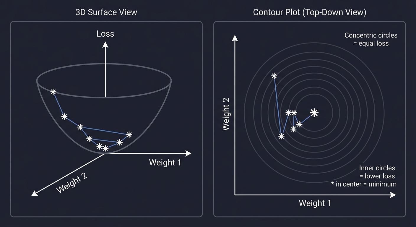
The Loss Landscape Visualization
For a simple 2-weight model, we can visualize the loss surface:
3D Surface View (Bowl Shape):

              Loss
               │
               │    * *
               │   *   *
               │  *     *
               │ *       *
               │*         *
               *───────────*──► Weight 1
              /
             /
            ▼
         Weight 2


Contour Plot View (Top-Down):

        Weight 2
           ^
           │    ....
           │  .      .
           │ .  ....  .
           │.  .    .  .
           │  .  ..  .  .
           │ .  .  .  .  .
           │.  .    .  .
           │ .  ....  .
           │  .      .
           │    ....
           └────────────────► Weight 1

           Concentric circles = equal loss
           Inner circles = lower loss
           * in center = minimum
Mathematical Derivation of Gradient Descent
Starting from a point x_0, we want to move to reduce f(x).
Taylor series approximation (first order):
f(x + delta) ≈ f(x) + gradient(f) . delta
We want f(x + delta) < f(x), so we want:
gradient(f) . delta < 0
The most negative value of a dot product is achieved when the vectors point in opposite directions. So:
delta = -alpha * gradient(f)
Where alpha > 0 is the learning rate.
The Update Rule:
x_new = x_old - alpha * gradient_f(x_old)

Or in component form for f(x, y):
    x_new = x_old - alpha * (df/dx)
    y_new = y_old - alpha * (df/dy)
Convergence Conditions
Gradient descent converges when:
- The function is convex (guarantees unique minimum)
- The gradient is Lipschitz continuous (bounded rate of change)
- The learning rate is small enough:
alpha < 2 / Lwhere L is the Lipschitz constant
For non-convex functions (like neural networks), we can only guarantee finding a stationary point (gradient = 0), which might be a local minimum or saddle point.
Convergence Check in Practice:

    if |gradient| < epsilon:
        print("Converged!")

    Or:

    if |loss_new - loss_old| < epsilon:
        print("Loss stopped changing!")
Real World Outcome
When you complete this project, running your visualizer will produce:
$ python descent.py --func "x^2 + y^2" --lr 0.1 --start "3,4"

=== GRADIENT DESCENT VISUALIZER ===
Function: f(x, y) = x^2 + y^2
Learning Rate: 0.1
Starting Point: (3.000, 4.000)
Convergence Threshold: 1e-6

Step | x        | y        | Loss      | Gradient       | Grad Magnitude
-----|----------|----------|-----------|----------------|---------------
  0  | 3.000000 | 4.000000 | 25.000000 | [6.00, 8.00]   | 10.000000
  1  | 2.400000 | 3.200000 | 16.000000 | [4.80, 6.40]   | 8.000000
  2  | 1.920000 | 2.560000 | 10.240000 | [3.84, 5.12]   | 6.400000
  3  | 1.536000 | 2.048000 | 6.553600  | [3.07, 4.10]   | 5.120000
  4  | 1.228800 | 1.638400 | 4.194304  | [2.46, 3.28]   | 4.096000
  5  | 0.983040 | 1.310720 | 2.684355  | [1.97, 2.62]   | 3.276800
  ...
 45  | 0.000347 | 0.000463 | 0.000000  | [0.00, 0.00]   | 0.000001

CONVERGED after 45 steps!
Final position: x=0.000347, y=0.000463
Final loss: 0.000000335

[Opening visualization window...]
The Visualization:
+------------------------------------------------------------------+
|  3D Surface Plot                |  Contour Plot with Path         |
|                                 |                                  |
|         /\                      |       . . . .                    |
|        /  \                     |     .   * * *   .                |
|       /    \                    |    .  * START *  .               |
|      /  **  \                   |   . *   \       *  .             |
|     /  *  *  \                  |  . *     \       *  .            |
|    / *    * \ \                 |  .*       \       *.             |
|   / *      *  \ \               |  .*        \      *.             |
|  /*          *\ \               |  . *        \    * .             |
| *------------*---\              |   . *       END * .              |
|                                 |    .  * * * *   .                |
|                                 |      . . . . .                   |
+------------------------------------------------------------------+
|  Learning Rate Comparison                                         |
|                                                                    |
|  lr=0.01: ------> very slow, many steps                          |
|  lr=0.1:  -> -> -> good convergence                              |
|  lr=0.5:  <-><-><-> oscillating, overshooting                    |
|  lr=1.0:  <-----> DIVERGING!                                      |
+------------------------------------------------------------------+
Solution Architecture
Before writing code, design the system:
┌─────────────────────────────────────────────────────────────────────┐
│                     GRADIENT DESCENT VISUALIZER                      │
├─────────────────────────────────────────────────────────────────────┤
│                                                                      │
│   ┌─────────────────┐     ┌─────────────────┐     ┌──────────────┐ │
│   │  Function       │     │   Gradient      │     │   Descent    │ │
│   │  Parser         │────▶│   Calculator    │────▶│   Engine     │ │
│   └─────────────────┘     └─────────────────┘     └──────────────┘ │
│          │                        │                      │          │
│          │                        │                      │          │
│          ▼                        ▼                      ▼          │
│   ┌─────────────────────────────────────────────────────────────┐  │
│   │                    History Collector                         │  │
│   │   [ (x0,y0,z0,grad0), (x1,y1,z1,grad1), ... ]                │  │
│   └─────────────────────────────────────────────────────────────┘  │
│                               │                                     │
│                               ▼                                     │
│   ┌─────────────────────────────────────────────────────────────┐  │
│   │                    Visualization Engine                      │  │
│   │   ┌─────────────┐  ┌─────────────┐  ┌─────────────────────┐ │  │
│   │   │ 3D Surface  │  │ Contour     │  │ Learning Rate       │ │  │
│   │   │ Plot        │  │ with Path   │  │ Comparison          │ │  │
│   │   └─────────────┘  └─────────────┘  └─────────────────────┘ │  │
│   └─────────────────────────────────────────────────────────────┘  │
│                                                                      │
└─────────────────────────────────────────────────────────────────────┘
Core Components
| Component | Responsibility | Input | Output |
|---|---|---|---|
| FunctionParser | Parse string like “x^2 + y^2” into callable function | String | Callable[[float, float], float] |
| GradientCalculator | Compute gradient numerically or symbolically | Function, Point | Gradient vector |
| DescentEngine | Execute the descent loop | Function, Gradient, Start, LR | History of points |
| Visualizer | Plot surfaces, contours, paths | History, Function | Matplotlib figures |
Data Structures
Point:
    x: float
    y: float

GradientVector:
    dx: float
    dy: float

HistoryEntry:
    step: int
    point: Point
    loss: float
    gradient: GradientVector
    gradient_magnitude: float

DescentHistory:
    entries: List[HistoryEntry]
    converged: bool
    final_step: int
Phased Implementation Guide
Phase 1: Function Definition and Parsing
Goal: Accept a mathematical expression and convert it to executable code.
Approach 1: Hardcoded Functions (Simpler)
FUNCTIONS = {
    "bowl": lambda x, y: x**2 + y**2,
    "rosenbrock": lambda x, y: (1-x)**2 + 100*(y-x**2)**2,
    "saddle": lambda x, y: x**2 - y**2,
}
Approach 2: Simple Parser (Intermediate)
- Replace
^with** - Use
eval()with safety restrictions - Parse into an AST for the brave
Key Questions:
- How will you handle invalid input?
- What functions will you support initially?
- How will you make the gradient calculation work with custom functions?
Deliverable: A module that takes a string and returns a callable f(x, y) -> z.
Phase 2: Gradient Calculation
Goal: Compute the gradient vector at any point.
Two Approaches:
Numerical Gradient (Finite Differences):
df/dx ≈ (f(x + h, y) - f(x - h, y)) / (2h)
df/dy ≈ (f(x, y + h) - f(x, y - h)) / (2h)

Where h is a small number like 1e-5
Pros: Works for ANY function Cons: Approximate, slow, numerical stability issues
Analytical Gradient (Symbolic): For known functions, compute the derivative by hand:
f(x, y) = x^2 + y^2
gradient = [2x, 2y]  <- you code this directly
Pros: Exact, fast Cons: You must derive and code each function’s gradient
Deliverable: A function gradient(f, x, y) -> (dx, dy) that returns the gradient vector.
Phase 3: The Descent Loop
Goal: Implement the core algorithm.
Pseudocode:
function gradient_descent(f, start, lr, max_steps, tolerance):
    x, y = start
    history = []

    for step in range(max_steps):
        loss = f(x, y)
        grad = gradient(f, x, y)
        grad_magnitude = sqrt(grad[0]^2 + grad[1]^2)

        history.append({step, x, y, loss, grad, grad_magnitude})

        if grad_magnitude < tolerance:
            return history, CONVERGED

        x = x - lr * grad[0]
        y = y - lr * grad[1]

    return history, NOT_CONVERGED
Key Decisions:
- When to stop? (Max steps? Gradient < threshold? Loss change < threshold?)
- How to handle divergence (loss -> infinity)?
- Should you track momentum? (Extension topic)
Deliverable: A function that runs descent and returns the full history.
Phase 4: Visualization with Matplotlib
Goal: Create stunning plots that reveal what’s happening.
Plot 1: 3D Surface
# Create a grid of x, y values
# Compute z = f(x, y) for each
# Use ax.plot_surface()
# Overlay the descent path with ax.plot()
Plot 2: Contour Map with Path
# Create contour lines with ax.contour() or ax.contourf()
# Plot the path as points + line
# Add arrows showing gradient direction
Plot 3: Loss Over Steps
# Simple line plot of loss vs step number
# Shows convergence behavior
Pro Tips:
- Use
plt.ion()for interactive mode during debugging - Save figures as PNG for the CLI workflow
- Add annotations (start point, end point, step numbers)
Deliverable: A visualization module that takes history and produces figures.
Phase 5: Learning Rate Experiments
Goal: Show how learning rate affects convergence.
Experiments to Implement:
- Side-by-Side Comparison
- Run descent with lr=0.01, 0.1, 0.5, 1.0
- Plot all paths on the same contour map
- Show which converges fastest
- Loss Curves Overlay
- Plot loss vs step for each learning rate
- Observe: slow convergence, good convergence, oscillation, divergence
- Animation (Bonus)
- Create a GIF or video of the ball rolling
- Use matplotlib.animation
Deliverable: A comparison mode that demonstrates learning rate effects.
Questions to Guide Your Design
Before you start coding, answer these in writing:
-
Why does taking the NEGATIVE gradient lead to the minimum? Hint: What does the gradient vector point toward?
-
If the gradient at (3, 4) for f(x,y) = x^2 + y^2 is [6, 8], what’s the magnitude? Follow-up: What’s the unit vector pointing downhill?
-
What happens if learning rate = 1.0 for f(x,y) = x^2 + y^2 starting at (1, 0)? Try it manually: x_new = 1 - 1.0 * 21 = ?*
-
Why can’t we just use learning_rate = infinity and get to the minimum in one step? Think about the Taylor approximation’s validity…
-
For f(x,y) = x^2 + 10y^2, should x and y converge at the same rate? This relates to conditioning and why Adam optimizer exists.
-
How would you detect if the algorithm is oscillating instead of converging? What pattern would you see in the history?
Thinking Exercise: Manual Gradient Descent on Paper
Before coding, work through this by hand:
Function: f(x, y) = x^2 + y^2
Starting point: (2.0, 3.0)
Learning rate: 0.1

STEP 0:
    Current: x=2.0, y=3.0
    Loss: f(2, 3) = 4 + 9 = 13
    Gradient: [2*2, 2*3] = [4, 6]
    Update: x_new = 2.0 - 0.1*4 = ____
            y_new = 3.0 - 0.1*6 = ____

STEP 1:
    Current: x=____, y=____
    Loss: f(__, __) = ____
    Gradient: [2*__, 2*__] = [__, __]
    Update: x_new = ____ - 0.1*____ = ____
            y_new = ____ - 0.1*____ = ____

STEP 2:
    Continue...

Questions:
- Is the loss decreasing each step?
- What's the pattern in how x and y change?
- Roughly how many steps to get loss < 0.01?
Answers to verify your work:
Step 0: (2.0, 3.0) -> (1.6, 2.4), loss 13 -> 8.32
Step 1: (1.6, 2.4) -> (1.28, 1.92), loss 8.32 -> 5.33
Step 2: (1.28, 1.92) -> (1.024, 1.536), loss 5.33 -> 3.41
Notice: Loss decreases by factor of 0.64 each step (for this function with this lr).
Testing Strategy
Unit Tests
Test 1: Gradient Calculation
    Input: f = x^2 + y^2, point = (1, 2)
    Expected: gradient = [2, 4]
    Tolerance: 1e-5 (for numerical gradient)

Test 2: Single Descent Step
    Input: f = x^2 + y^2, point = (1, 0), lr = 0.5
    Expected: new point = (0, 0)  # Happens to hit minimum exactly!

Test 3: Convergence on Simple Bowl
    Input: f = x^2 + y^2, start = (5, 5), lr = 0.1
    Expected: converges to (0, 0) within 100 steps

Test 4: Divergence Detection
    Input: f = x^2 + y^2, start = (1, 1), lr = 2.0
    Expected: loss > 1000 within 10 steps (diverging!)

Test 5: Saddle Point Behavior
    Input: f = x^2 - y^2, start = (0.1, 0.1), lr = 0.1
    Expected: converges to (0, ?) but y keeps growing
Visual Validation
Create these known test cases and verify they look right:
- Bowl (x^2 + y^2): Straight path to center
- Ellipse (x^2 + 10*y^2): Zig-zag path (y converges faster)
- Rosenbrock: Curved path following the banana valley
- Saddle (x^2 - y^2): Approaches origin, then escapes
Edge Cases
- Start at the minimum: Should immediately converge
- Start at a saddle point: Gradient is zero, might get stuck
- Very large starting point: Numerical overflow possible
- Zero learning rate: No movement at all
Common Pitfalls and Debugging Tips
Pitfall 1: Numerical Gradient Instability
Symptom: Gradient values seem wrong or noisy
Cause: Finite difference step size h is too large or too small
Fix:
# Too small: floating point cancellation
h = 1e-15  # BAD!

# Too large: approximation is inaccurate
h = 1.0    # BAD!

# Just right: balance precision and accuracy
h = 1e-5   # GOOD
Pitfall 2: Forgetting the Negative
Symptom: The ball rolls UPHILL
Cause: x = x + lr * grad instead of x = x - lr * grad
Check: After one step, loss should decrease (for convex functions).
Pitfall 3: Mutating Instead of Creating New Values
Symptom: History shows same point repeated
Cause:
# BAD: modifying list in place
point[0] -= lr * grad[0]
history.append(point)  # Appends reference to same list!

# GOOD: create new values
x_new = point[0] - lr * grad[0]
history.append((x_new, y_new))
Pitfall 4: Overflow with Aggressive Learning Rate
Symptom: inf or nan values appear
Cause: Learning rate too high, values explode
Fix:
if loss > 1e10:
    print("DIVERGENCE DETECTED! Reduce learning rate.")
    break
Pitfall 5: Convergence Check Too Strict
Symptom: Never reports convergence despite loss being tiny
Cause: Checking gradient == 0 exactly (floating point never equals exactly 0)
Fix:
# BAD
if gradient_magnitude == 0:

# GOOD
if gradient_magnitude < 1e-6:
The Interview Questions They’ll Ask
When you understand this project, you can answer these common interview questions:
Q1: “What is gradient descent?”
Answer: Gradient descent is an iterative optimization algorithm that finds local minima of differentiable functions by repeatedly taking steps in the direction opposite to the gradient (steepest descent direction).
Q2: “How do you choose the learning rate?”
Answer: The learning rate is typically chosen empirically. Too small = slow convergence. Too large = oscillation or divergence. Common strategies include: starting with 0.01 or 0.001, learning rate schedules (decay over time), adaptive methods like Adam that adjust per-parameter.
Q3: “What’s the difference between batch, mini-batch, and stochastic gradient descent?”
Answer:
- Batch GD: Compute gradient using ALL training examples
- Mini-batch GD: Compute gradient using a subset (e.g., 32 examples)
- Stochastic GD (SGD): Compute gradient using ONE example at a time Mini-batch is most common as it balances computation efficiency and gradient noise.
Q4: “What is a local minimum vs global minimum?”
Answer: A local minimum is a point where all nearby points have higher values, but there may be lower points elsewhere. A global minimum is the absolute lowest point. Neural networks have many local minima, but research suggests many are “good enough.”
Q5: “What is the problem with vanilla gradient descent, and how does momentum help?”
Answer: Vanilla GD can oscillate in “ravines” (directions with steep vs gentle slopes) and get stuck. Momentum accumulates past gradients like a rolling ball, helping it power through oscillations and flat regions.
Q6: “Why do we use automatic differentiation instead of numerical differentiation?”
Answer: Numerical differentiation is: (1) approximate due to finite differences, (2) slow because it requires function evaluations per variable, (3) numerically unstable. Autodiff is exact, efficient, and stable by applying chain rule symbolically.
Hints in Layers
If you get stuck, reveal these hints one at a time:
Hint 1: Function Structure
Your main file should have this structure:
def f(x, y):
    # The function to minimize
    pass

def gradient(x, y):
    # Returns [df/dx, df/dy]
    pass

def descent(f, grad, start_x, start_y, lr, max_steps):
    # The main loop
    pass

def visualize(history):
    # Matplotlib code
    pass

if __name__ == "__main__":
    # Parse args, run descent, show plots
    pass
Hint 2: Numerical Gradient Implementation
def numerical_gradient(f, x, y, h=1e-5):
    df_dx = (f(x + h, y) - f(x - h, y)) / (2 * h)
    df_dy = (f(x, y + h) - f(x, y - h)) / (2 * h)
    return [df_dx, df_dy]
Hint 3: Descent Loop Core
x, y = start_x, start_y
history = [(x, y, f(x, y))]

for step in range(max_steps):
    grad = gradient(x, y)
    x = x - lr * grad[0]
    y = y - lr * grad[1]
    history.append((x, y, f(x, y)))

    if abs(grad[0]) < 1e-6 and abs(grad[1]) < 1e-6:
        break

return history
Hint 4: Basic Contour Plot
import numpy as np
import matplotlib.pyplot as plt

# Create grid
x_vals = np.linspace(-5, 5, 100)
y_vals = np.linspace(-5, 5, 100)
X, Y = np.meshgrid(x_vals, y_vals)
Z = X**2 + Y**2  # Your function

# Contour plot
plt.contour(X, Y, Z, levels=20)

# Path overlay
path_x = [h[0] for h in history]
path_y = [h[1] for h in history]
plt.plot(path_x, path_y, 'r.-', markersize=10)

plt.show()
Hint 5: 3D Surface Plot
from mpl_toolkits.mplot3d import Axes3D

fig = plt.figure()
ax = fig.add_subplot(111, projection='3d')

# Surface
ax.plot_surface(X, Y, Z, alpha=0.5, cmap='viridis')

# Path
path_z = [h[2] for h in history]
ax.plot(path_x, path_y, path_z, 'r.-', markersize=10, linewidth=2)

plt.show()
Extensions and Challenges
Once basic gradient descent works, try these:
Extension 1: Implement Momentum
velocity = 0
for each step:
    velocity = momentum * velocity + lr * gradient
    x = x - velocity
Momentum helps the optimizer “roll through” flat regions and oscillations.
Extension 2: Add the Rosenbrock Function
f(x, y) = (1 - x)^2 + 100 * (y - x^2)^2
This banana-shaped function is a classic optimization test. It has a narrow curved valley - watch how vanilla GD struggles!
Rosenbrock Contour (The Banana):

     y
     ^
     |    * * * * * * *
     |   *           *
     |  *           *
     | *           *    <- The valley curves
     |*  Minimum  *
     | *   here  *
     |  * * * * *
     └──────────────────► x
Extension 3: Side-by-Side Learning Rate Comparison
Run 4 experiments with lr = [0.001, 0.01, 0.1, 0.5] and plot all paths on the same figure with a legend.
Extension 4: Implement Adam Optimizer
Adam combines momentum with per-parameter adaptive learning rates:
m = beta1 * m + (1 - beta1) * gradient
v = beta2 * v + (1 - beta2) * gradient^2
m_hat = m / (1 - beta1^t)
v_hat = v / (1 - beta2^t)
x = x - lr * m_hat / (sqrt(v_hat) + epsilon)
Compare Adam to vanilla GD on the Rosenbrock function.
Extension 5: Animation
Use matplotlib.animation.FuncAnimation to create a GIF of the descent process.
Extension 6: N-Dimensional Generalization
Extend your code to work with functions of N variables (e.g., f(x1, x2, …, xn)). You won’t be able to visualize it, but you can plot loss vs steps.
Real-World Connections
This IS How Neural Networks Train
When you call model.fit() in TensorFlow or loss.backward() in PyTorch, this is exactly what’s happening:
- Forward pass: compute predictions and loss
- Backward pass: compute gradients (via backpropagation)
- Update step:
weights -= learning_rate * gradients
The only differences are:
- Millions of parameters instead of 2
- Automatic differentiation instead of manual/numerical gradients
- Sophisticated optimizers (Adam, SGD with momentum)
- Mini-batches instead of full dataset
Loss Landscapes in Practice
Real neural network loss landscapes have been visualized:
What we imagine:        What it actually looks like:

    Nice bowl               Chaotic terrain

      /\                       /\  /\
     /  \                   /\/  \/  \/\
    /    \                 /            \
   /      \               /    ___       \
  /        \             /    /   \       \

Good news: Many local minima are "good enough" in practice!
Why Learning Rate Matters in Production
- Too high: Training diverges, model is useless
- Too low: Training takes days instead of hours ($$$)
- Just right: Fast convergence to good solution
This is why hyperparameter tuning (finding the right lr) is a major part of ML engineering.
Books That Will Help
| Book | Chapter | What You’ll Learn |
|---|---|---|
| “Deep Learning” by Goodfellow et al. | Ch. 4: Numerical Computation | Mathematical foundations of optimization |
| “Deep Learning” by Goodfellow et al. | Ch. 8: Optimization | Adam, momentum, learning rate schedules |
| “Grokking Deep Learning” by Andrew Trask | Ch. 4-5 | Intuitive explanations with Python code |
| “Calculus Made Easy” by Silvanus Thompson | All | If you need a calculus refresher |
Online Resources:
- Andrej Karpathy’s CS231n lecture notes on optimization
- Distill.pub articles on momentum and Adam
- 3Blue1Brown’s “Essence of Calculus” YouTube series
Self-Assessment Checklist
Before considering this project complete, verify:
Understanding
- I can explain why the gradient points uphill
- I can manually compute the gradient of
f(x,y) = x^2 + 3xy + y^2 - I understand why learning rate = 1.0 causes problems for
f(x) = x^2 - I can explain the difference between local and global minima
- I know what a saddle point is and why it’s problematic
Implementation
- My gradient calculation matches analytical derivatives (within tolerance)
- Descent converges to (0, 0) for
f(x, y) = x^2 + y^2within 100 steps - My code detects and reports divergence
- I can visualize the descent path on a contour plot
- I can show side-by-side comparison of different learning rates
Extensions
- I implemented momentum and observed the difference
- I tested on the Rosenbrock function
- I can explain why Adam works better than vanilla GD in most cases
Interview Ready
- I can whiteboard the gradient descent algorithm
- I can discuss trade-offs of batch vs stochastic gradient descent
- I can explain how this relates to neural network training
What’s Next?
After completing this project, you’re ready for:
- Project 3: Linear Regression Engine - Apply gradient descent to actual data
- Project 5: Autograd Engine - Automate the gradient calculation
- Deep dive into optimizers - Study Adam, RMSprop, AdaGrad
The gradient descent visualizer is your foundation. Every future project builds on the intuition you’ve developed here: loss surfaces, gradients, learning rates, and convergence. When you train a 100-million parameter model and it diverges, you’ll know exactly what went wrong - because you watched the ball roll off the edge of the bowl.
“The gradient is not just a number. It’s a compass pointing toward failure. Go the opposite direction.”