Project 8: Symbolic Derivative Calculator

A program that takes a mathematical expression like x^3 + sin(x*2) and outputs its exact symbolic derivative: 3*x^2 + 2*cos(x*2).

Quick Reference

Attribute	Value
Difficulty	Level 2: Intermediate (The Developer)
Main Programming Language	Python
Alternative Programming Languages	Haskell, Lisp, Rust
Coolness Level	Level 3: Genuinely Clever
Business Potential	1. The “Resume Gold” (Educational/Personal Brand)
Knowledge Area	Symbolic Computation / Calculus
Software or Tool	Symbolic Differentiator
Main Book	“Structure and Interpretation of Computer Programs” by Abelson & Sussman

---

1. Learning Objectives

By completing this project, you will:

1. Translate math definitions into deterministic implementation steps.
2. Build validation checks that make correctness observable.
3. Diagnose numerical, logical, and data-shape failures early.
4. Explain tradeoffs in interviews using evidence from your own build.

---

2. All Theory Needed (Per-Concept Breakdown)

This project applies the following theory clusters:

• Symbolic-to-numeric translation (expressions, data shapes, invariants)
• Stability constraints (precision, scaling, stopping criteria)
• Optimization or inference logic (depending on project objective)
• Evaluation discipline (error analysis, test coverage, reproducibility)

Concept A: Mathematical Representation Discipline

Fundamentals A math expression is not executable until you define representation, ordering, and domain constraints. The same equation can be represented as a token stream, tree, matrix pipeline, or probability graph. Choosing representation determines what bugs you can catch early.

Deep Dive into the concept Most project failures begin before algorithm selection: they start with ambiguous representation. If your parser cannot distinguish unary minus from subtraction, your calculator fails. If your matrix dimensions are implicit rather than validated, your linear algebra pipeline fails silently. If your probabilistic assumptions (independence, stationarity, or class priors) are not explicit, your inference can look accurate on one split and collapse on another. The core implementation move is to treat representation as a contract. Define each object with shape, domain, and semantic intent. Then enforce invariants at boundaries: input parser, preprocessing, training loop, evaluation stage. This makes debugging local instead of global.

How this fits this project You will encode each operation with explicit contracts and invariant checks.

Definitions & key terms

• Invariant: Property that must hold before and after each operation.
• Shape contract: Expected dimensional structure of vectors/matrices/tensors.
• Domain constraint: Allowed value range (for example log input > 0).

Mental model diagram

User Input -> Representation Layer -> Validated Operation -> Observable Output
              (tokens/shapes)        (invariants pass)       (tests/plots/logs)

How it works

1. Parse/ingest data into typed structures.
2. Validate shape/domain invariants.
3. Execute operation.
4. Compare observed output with expected behavior.
5. Record failure signature if mismatch appears.

Minimal concrete example

PSEUDOCODE
read expression
tokenize with precedence rules
if token sequence invalid -> return syntax error
evaluate tree
if domain violation -> return bounded diagnostic
print value and confidence check

Common misconceptions

• “If it runs once, representation is correct.” -> false.
• “Type checks are enough without shape checks.” -> false.

Check-your-understanding questions

1. Which invariant catches division-by-zero earliest?
2. Why does shape validation belong at boundaries rather than only in core logic?
3. Predict failure if tokenization ignores unary minus.

Check-your-understanding answers

1. Domain check on denominator before operation execution.
2. Boundary validation keeps errors local and diagnostic.
3. Expressions like -2^2 get misinterpreted and produce wrong precedence behavior.

Real-world applications Feature preprocessing, model-serving input validation, and experiment-tracking schema enforcement.

Where you’ll apply it This project and every downstream project in the sprint.

References

• CSAPP (Bryant & O’Hallaron), floating-point chapter
• Math for Programmers (Paul Orland), representation-oriented chapters

Key insight Correct representation reduces the complexity of every later decision.

Summary Stable ML math implementations start with explicit contracts, not implicit assumptions.

Homework/Exercises

1. Write five invariants for your project.
2. Build a failing test input for each invariant.

Solutions

1. Include at least one shape, one domain, one convergence, one reproducibility, and one output-range invariant.
2. Each failing input should trigger exactly one diagnostic to keep root-cause analysis clean.

---

3. Build Blueprint

1. Scope the smallest end-to-end slice that produces visible output.
2. Add deterministic tests and edge-case probes.
3. Layer complexity only after baseline behavior is stable.
4. Add metrics logging before optimization.
5. Run failure drills: perturb inputs, scale values, and check stability.

---

4. Real-World Outcome (Target)

$ python derivative.py "x^3"
d/dx(x³) = 3·x²

$ python derivative.py "sin(x) * cos(x)"
d/dx(sin(x)·cos(x)) = cos(x)·cos(x) + sin(x)·(-sin(x))
                    = cos²(x) - sin²(x)
                    = cos(2x)  [after simplification]

$ python derivative.py "exp(x^2)"
d/dx(exp(x²)) = exp(x²) · 2x  [chain rule applied!]

$ python derivative.py "log(sin(x))"
d/dx(log(sin(x))) = (1/sin(x)) · cos(x) = cos(x)/sin(x) = cot(x)

Implementation Hints: Represent expressions as trees. For x^3 + sin(x):

        +
       / \
      ^   sin
     / \    \
    x   3    x

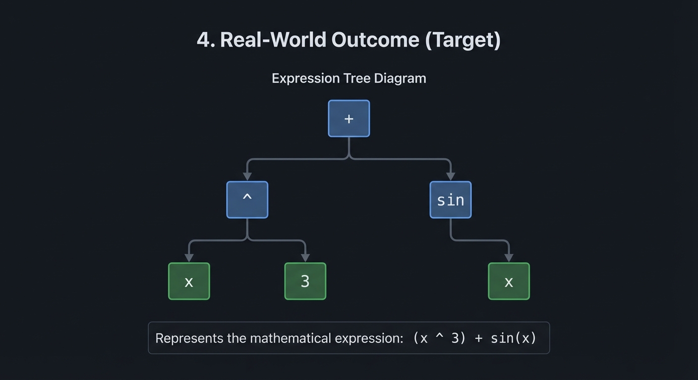
Derivative rules become recursive tree transformations:

• deriv(x) = 1
• deriv(constant) = 0
• deriv(a + b) = deriv(a) + deriv(b)
• deriv(a * b) = deriv(a)*b + a*deriv(b) [product rule]
• deriv(f(g(x))) = deriv_f(g(x)) * deriv(g(x)) [chain rule]

The chain rule is crucial for ML: backpropagation is just the chain rule applied repeatedly!

Learning milestones:

1. Polynomial derivatives work → You’ve mastered the power rule
2. Product and quotient rules work → You understand how derivatives distribute
3. Chain rule handles nested functions → You understand composition (critical for backprop!)

---

5. Core Design Notes from Main Guide

Core Question

How can a computer manipulate mathematical symbols rather than just numbers, and why is the chain rule the secret to computing derivatives of any composed function?

Numeric computation deals with specific values; symbolic computation deals with abstract expressions. When you implement symbolic differentiation, you are teaching a computer to apply the rules of calculus that you learned by hand. The chain rule is the master key: any complicated function is just simple functions nested inside each other, and the chain rule tells you how to peel back the layers. This is not just an exercise–automatic differentiation (used in every deep learning framework) is a descendant of these ideas.

Concepts You Must Understand First

Stop and research these before coding:

1. Expression trees and recursive structure of mathematical expressions
   • Why is 3 + 4 * 5 naturally represented as a tree?
   • How does the tree structure encode operator precedence?
   • Why is recursion the natural way to evaluate and transform expression trees?
   • Book Reference: “SICP” Section 2.3.2 - Abelson & Sussman
2. The derivative rules and when to apply each
   • Power rule: d/dx[x^n] = n*x^(n-1)
   • Sum rule: d/dx[f+g] = df/dx + dg/dx
   • Product rule: d/dx[f*g] = f’g + fg’
   • Quotient rule: d/dx[f/g] = (f’g - fg’)/g^2
   • Book Reference: “Calculus” Chapter 3 - James Stewart
3. The chain rule: the key to composed functions
   • If y = f(g(x)), then dy/dx = f’(g(x)) * g’(x)
   • Why multiply the derivatives? Think about rates of change.
   • How to apply the chain rule to triple composition f(g(h(x)))?
   • Book Reference: “Calculus” Chapter 3.4 - James Stewart
4. Derivatives of transcendental functions
   • d/dx[sin(x)] = cos(x)
   • d/dx[cos(x)] = -sin(x)
   • d/dx[exp(x)] = exp(x)
   • d/dx[ln(x)] = 1/x
   • Book Reference: “Math for Programmers” Chapter 8 - Paul Orland
5. Expression simplification: a hard problem
   • Why does derivative output often look ugly (0x + 1y)?
   • What simplification rules help? (0x = 0, 1x = x, x+0 = x)
   • Why is full algebraic simplification actually very hard?
   • Book Reference: “Computer Algebra” Chapter 1 - Geddes et al.

Questions to Guide Your Design

Before implementing, think through these:

1. How will you represent expressions? Classes for each operator type? Nested tuples? Strings with parsing? Each has trade-offs.

2. How will you distinguish x from constants? You need to know that d/dx[x] = 1 but d/dx[3] = 0. How is this represented?

3. How will you handle the chain rule? When you encounter sin(2x), you need to recognize it as sin(u) where u = 2x, compute d/du[sin(u)] = cos(u), then multiply by du/dx = 2.

4. What is your simplification strategy? Simplify during differentiation? After? Recursively? How much simplification is “enough”?

5. How will you output the result? As a new expression tree? As a string? In what notation?

6. How will you test correctness? Compare symbolic result to numerical derivative at random points?

Thinking Exercise

Before writing any code, manually trace the derivative of sin(x^2):

Expression tree:
    sin
     |
    pow
    / \
   x   2

Step 1: Recognize this is sin(u) where u = x^2
        Need chain rule: d/dx[sin(u)] = cos(u) * du/dx

Step 2: Compute d/du[sin(u)] = cos(u) = cos(x^2)

Step 3: Compute du/dx = d/dx[x^2]
        This is pow(x, 2), apply power rule: 2*x^1 = 2*x

Step 4: Apply chain rule: cos(x^2) * 2*x

Step 5: Simplify (optional): 2*x*cos(x^2)

Result tree:
        *
       / \
      2   *
         / \
        x  cos
            |
           pow
           / \
          x   2

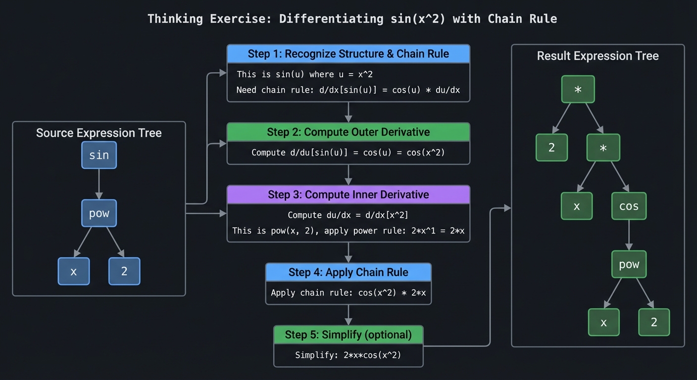
Now verify numerically: at x=1, derivative should be 21cos(1) = 1.08. Numerical approximation: (sin(1.001^2) - sin(0.999^2)) / 0.002 = 1.08. Correct!

Interview Questions

1. “How would you implement a symbolic derivative calculator?” Expected answer: Represent expressions as trees, apply derivative rules recursively. The chain rule handles function composition.

2. “Walk me through differentiating exp(x^2) symbolically.” Expected answer: This is exp(u) where u = x^2. Derivative of exp(u) is exp(u). Derivative of x^2 is 2x. By chain rule: exp(x^2) * 2x = 2x*exp(x^2).

3. “What is the chain rule and why is it fundamental?” Expected answer: d/dx[f(g(x))] = f’(g(x)) * g’(x). It lets us differentiate any composed function by breaking it into inner and outer parts.

4. “How does symbolic differentiation differ from numerical differentiation?” Expected answer: Symbolic gives an exact formula; numerical gives an approximation at specific points. Symbolic is more general but harder to implement. Symbolic can be simplified; numerical cannot.

5. “What is the connection between symbolic differentiation and backpropagation?” Expected answer: Both apply the chain rule to compute derivatives of composed functions. Backprop is a form of automatic differentiation, which is related to but different from symbolic differentiation.

6. “How do you handle the product rule in an expression tree?” Expected answer: For ab, create a new tree: (deriv(a)b) + (a*deriv(b)). Recursively differentiate the subexpressions.

Hints in Layers (Treat as pseudocode guidance)

Hint 1: Use Python classes for your expression tree:

class Var:  # Represents x
    pass
class Const:  # Represents a number
    def __init__(self, value): self.value = value
class Add:
    def __init__(self, left, right): ...
class Mul:
    def __init__(self, left, right): ...
class Sin:
    def __init__(self, arg): ...

Hint 2: The derivative function is a big recursive pattern match:

def deriv(expr):
    if isinstance(expr, Var):
        return Const(1)
    elif isinstance(expr, Const):
        return Const(0)
    elif isinstance(expr, Add):
        return Add(deriv(expr.left), deriv(expr.right))
    elif isinstance(expr, Mul):
        # Product rule
        return Add(
            Mul(deriv(expr.left), expr.right),
            Mul(expr.left, deriv(expr.right))
        )
    # etc.

Hint 3: For chain rule (e.g., sin(f(x))):

elif isinstance(expr, Sin):
    # d/dx[sin(f)] = cos(f) * f'
    return Mul(Cos(expr.arg), deriv(expr.arg))

Hint 4: Basic simplification:

def simplify(expr):
    if isinstance(expr, Mul):
        left, right = simplify(expr.left), simplify(expr.right)
        if isinstance(left, Const) and left.value == 0:
            return Const(0)
        if isinstance(left, Const) and left.value == 1:
            return right
        # ... more rules

Hint 5: Test with numerical differentiation:

def numerical_deriv(f, x, eps=1e-7):
    return (f(x + eps) - f(x - eps)) / (2 * eps)

# Compare to your symbolic result evaluated at x

Books That Will Help

Topic	Book	Chapter
Expression Trees	“SICP” - Abelson & Sussman	Section 2.3
Derivative Rules	“Calculus” - James Stewart	Chapter 3
Chain Rule Deep Dive	“Calculus” - James Stewart	Chapter 3.4
Symbolic Computation	“Computer Algebra” - Geddes et al.	Chapter 1
Pattern Matching	“Language Implementation Patterns” - Terence Parr	Chapter 4
Automatic Differentiation	“Deep Learning” - Goodfellow et al.	Chapter 6
Practical Applications	“Math for Programmers” - Paul Orland	Chapter 8

---

---

6. Validation, Pitfalls, and Completion

Common Pitfalls and Debugging

Problem 1: “Outputs drift after a few iterations”

• Why: Hidden numerical instability (unscaled features, aggressive step size, or repeated subtraction of nearly equal values).
• Fix: Normalize inputs, reduce step size, and track relative error rather than only absolute error.
• Quick test: Run the same task with two scales of input (for example x and 10x) and compare normalized error curves.

Problem 2: “Results are inconsistent across runs”

• Why: Random seeds, data split randomness, or non-deterministic ordering are uncontrolled.
• Fix: Set seeds, log configuration, and store split indices and hyperparameters with each run.
• Quick test: Re-run three times with the same seed and confirm metrics remain inside a tight tolerance band.

Problem 3: “The project works on the demo case but fails on edge cases”

• Why: Tests only cover happy-path inputs.
• Fix: Add adversarial inputs (empty values, extreme ranges, near-singular matrices, rare classes).
• Quick test: Build an edge-case test matrix and ensure every scenario reports expected behavior.

Definition of Done

• Core functionality works on reference inputs
• Edge cases are tested and documented
• Results are reproducible (seeded and versioned configuration)
• Performance or convergence behavior is measured and explained
• A short retrospective explains what failed first and how you fixed it

---

7. Extension Ideas

1. Add a stress-test mode with adversarial inputs.
2. Add a short benchmark report (runtime + memory + error trend).
3. Add a reproducibility bundle (seed, config, and fixed test corpus).

8. Why This Project Matters

Not specified

This project is valuable because it creates observable evidence of mathematical reasoning under real implementation constraints.