Sprint: Math for Machine Learning Mastery - Real World Projects
Goal: Build deep, implementation-level mathematical intuition for machine learning by moving from symbolic reasoning to numerical reasoning and finally to model training decisions. You will learn why each math concept exists, where it breaks in practice, and how it surfaces in real ML systems. By the end, you will be able to explain and implement core ML math workflows without treating libraries as black boxes. You will also develop the judgment to debug instability, pick appropriate loss/optimization strategies, and defend your model choices in interviews or production reviews.
Introduction
Math for machine learning is the language that connects data, models, and decisions under uncertainty. In this guide, you will build projects that start with expression parsing and end with full pipeline evaluation, so each abstract concept becomes an observable artifact.
- What this solves today: Teams often ship models that “work” but fail under shift, scale, or noisy data because foundational math assumptions were never validated.
- What you will build: 31 projects covering algebra, linear algebra, calculus, probability/statistics, optimization, matrix calculus, information theory, numerical stability, convex optimization, and advanced ML math extensions.
- In scope: Mathematical modeling, numerical behavior, optimization dynamics, and model evaluation.
- Out of scope: Framework-specific production deployment infrastructure (Kubernetes, feature stores, CI/CD for ML services).
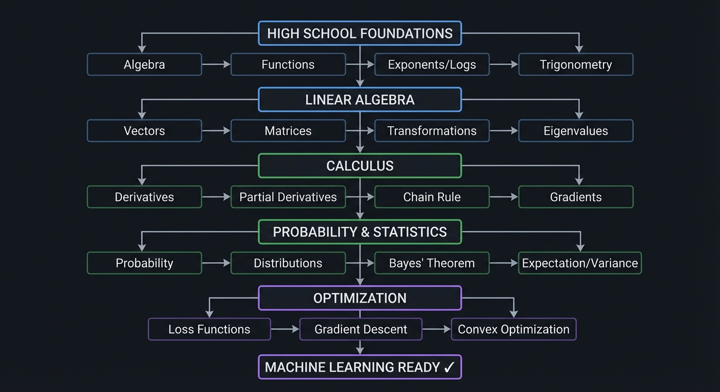
HIGH SCHOOL FOUNDATIONS
    ↓
    Algebra → Functions → Exponents/Logs → Trigonometry
    ↓
LINEAR ALGEBRA
    ↓
    Vectors → Matrices → Transformations → Eigenvalues
    ↓
CALCULUS
    ↓
    Derivatives → Partial Derivatives → Chain Rule → Gradients
    ↓
PROBABILITY & STATISTICS
    ↓
    Probability → Distributions → Bayes' Theorem → Expectation/Variance
    ↓
OPTIMIZATION
    ↓
    Loss Functions → Gradient Descent → Convex Optimization
    ↓
MACHINE LEARNING READY ✓
How to Use This Guide
- Read the Theory Primer first, concept by concept, and take notes on failure modes and invariants.
- Do projects in order unless you already have mastery in a cluster; each later cluster assumes execution confidence from earlier ones.
- For each project, answer the Core Question before implementation.
- Validate with the Definition of Done checklists and keep a project log (inputs, configs, errors, fixes, outcomes).
- Treat all snippets as pseudocode or implementation guides; translate them deliberately to your language/runtime.
Prerequisites & Background Knowledge
Essential Prerequisites (Must Have)
- Basic programming in one language (Python recommended for speed of iteration)
- Comfort with loops, conditionals, arrays/lists, and functions
- Basic CLI usage and package management
- Recommended Reading: “Math for Programmers” by Paul Orland - Chapters 1-3
Helpful But Not Required
- Basic plotting and data manipulation tools (Matplotlib, Pandas, GNUplot, or equivalents)
- Introductory statistics vocabulary
- Familiarity with Git and reproducible experiments
Self-Assessment Questions
- Can you explain why
log(exp(x)) = xbut domain constraints still matter in implementation? - Can you solve a 2x2 linear system and interpret the geometry of the solution?
- Can you explain what a gradient means in plain language and how it affects parameter updates?
Development Environment Setup Required Tools:
- Python 3.11+ or equivalent language runtime
- Plotting library (Matplotlib or equivalent)
- CSV/JSON parsing support
- Test runner (pytest or equivalent)
Recommended Tools:
- Jupyter Notebook or Quarto for experiment logs
jqfor result-file inspection- A fixed random seed utility and simple benchmarking script
Testing Your Setup:
$ python --version
Python 3.11.x
$ python -c "print('env ok')"
env ok
Time Investment
- Simple projects: 4-8 hours each
- Moderate projects: 10-20 hours each
- Complex projects: 20-40 hours each
- Total sprint: ~8-12 months (part-time)
Important Reality Check Progress is non-linear. The hardest part is not syntax; it is learning to map symbolic equations to robust numerical procedures under finite precision and noisy data.
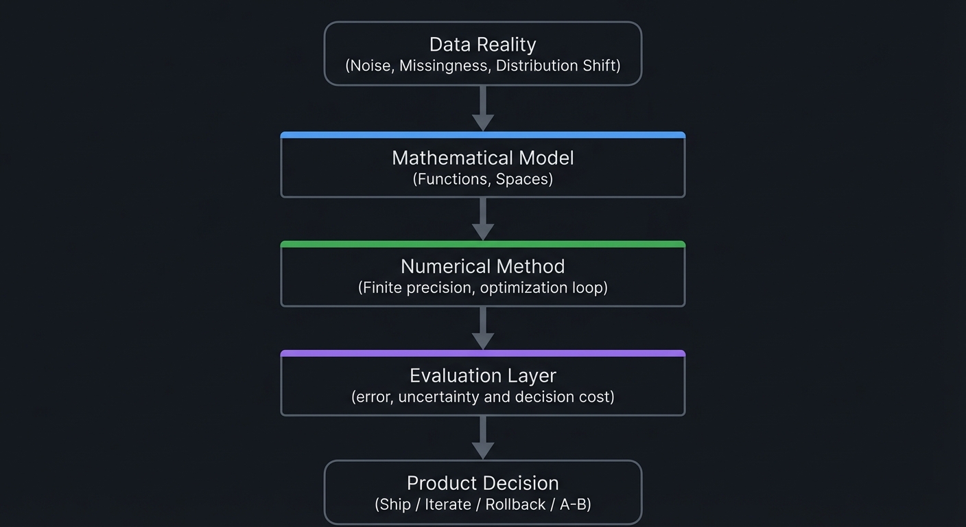
Big Picture / Mental Model
   Data Reality
(Noise, Missingness,
 Distribution Shift)
        |
        v
+--------------------+
| Mathematical Model |
| (Functions, Spaces)|
+--------------------+
        |
        v
+--------------------+
| Numerical Method   |
| (Finite precision, |
| optimization loop) |
+--------------------+
        |
        v
+--------------------+
| Evaluation Layer   |
| (error, uncertainty|
| and decision cost) |
+--------------------+
        |
        v
  Product Decision
 (Ship / Iterate /
   Rollback / A-B)
Theory Primer
This primer keeps theory and implementation coupled. Every concept includes mental models, invariants, and failure modes so you can diagnose behavior in real training workflows.
This section provides detailed explanations of the core mathematical concepts that all 31 projects in this guide teach. Understanding these concepts deeply—not just procedurally—will transform you from someone who uses ML libraries to someone who truly understands what happens inside them.
\1
Before diving into each mathematical area, let’s understand why these specific topics are essential:
┌─────────────────────────────────────────────────────────────────────────┐
│                    THE ML MATHEMATICS ECOSYSTEM                         │
├─────────────────────────────────────────────────────────────────────────┤
│                                                                         │
│  ALGEBRA                    LINEAR ALGEBRA              CALCULUS        │
│  ────────                   ──────────────              ────────        │
│  Variables as              Vectors & Matrices          Derivatives      │
│  unknowns we solve     ──▶ as data containers     ──▶  measure change   │
│  for in equations          & transformations          in predictions   │
│        │                         │                          │          │
│        │                         │                          │          │
│        ▼                         ▼                          ▼          │
│  ┌─────────────────────────────────────────────────────────────────┐   │
│  │                    OPTIMIZATION (GRADIENT DESCENT)              │   │
│  │         The algorithm that makes neural networks "learn"        │   │
│  │               by minimizing prediction errors                   │   │
│  └─────────────────────────────────────────────────────────────────┘   │
│        ▲                         ▲                          ▲          │
│        │                         │                          │          │
│  FUNCTIONS                 PROBABILITY              EXPONENTS/LOGS     │
│  ─────────                 ───────────              ──────────────     │
│  Map inputs to            Quantify uncertainty      Scale data,        │
│  outputs (the core        in predictions,           measure info,      │
│  of all ML models)        model noise               enable learning    │
│                                                                         │
└─────────────────────────────────────────────────────────────────────────┘
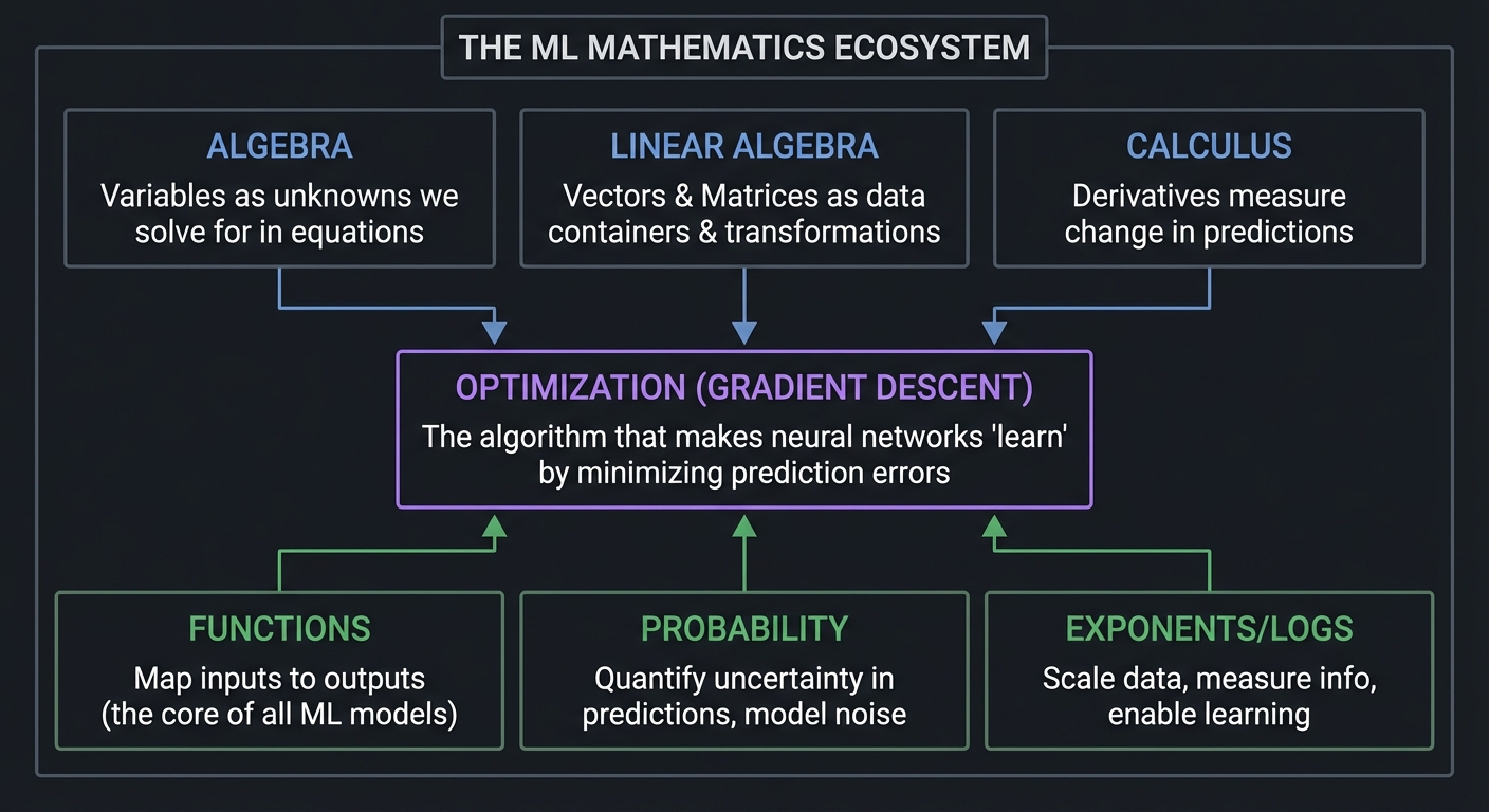
Every neural network is fundamentally:
- A composition of functions (algebra)
- Represented by matrices of weights (linear algebra)
- Trained by computing gradients (calculus)
- Making probabilistic predictions (probability)
- Optimized by gradient descent (optimization)
The math is not abstract theory—it is the actual implementation. When you run model.fit() in PyTorch or TensorFlow, these mathematical operations are exactly what happens inside.
\1
Algebra is the foundation upon which all higher mathematics rests. At its core, algebra is about expressing relationships between quantities using symbols, then manipulating those symbols to discover new truths.
Variables: Placeholders for Unknown or Changing Quantities
In ML, we use variables constantly:
xrepresents input features (a single number or a vector of thousands)yrepresents the target we want to predictw(weights) andb(bias) are the parameters we learnθ(theta) represents all learnable parameters
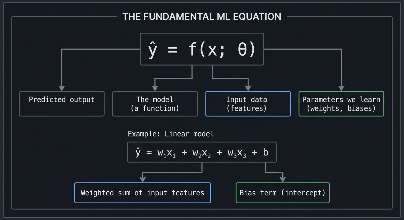
THE FUNDAMENTAL ML EQUATION

     ŷ = f(x; θ)
     │   │  │  │
     │   │  │  └── Parameters we learn (weights, biases)
     │   │  └───── Input data (features)
     │   └──────── The model (a function)
     └──────────── Predicted output

Example: Linear model
     ŷ = w₁x₁ + w₂x₂ + w₃x₃ + b
         └────────┬─────────┘   │
                  │             │
         Weighted sum of    Bias term
         input features     (intercept)
Equations: Statements of Equality We Solve
An equation states that two expressions are equal. Solving equations means finding values that make this true.
SOLVING A LINEAR EQUATION

Find x such that: 3x + 7 = 22

Step 1: Subtract 7 from both sides
        3x + 7 - 7 = 22 - 7
        3x = 15

Step 2: Divide both sides by 3
        3x/3 = 15/3
        x = 5

Verification: 3(5) + 7 = 15 + 7 = 22 ✓
In ML, we don’t solve single equations—we solve systems of equations represented as matrices, or we use iterative methods (gradient descent) to find approximate solutions.
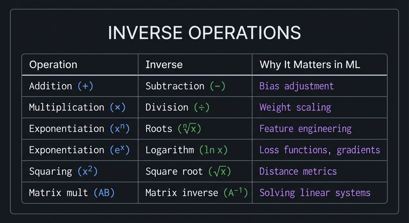
Inverse Operations: The Key to Solving
Every operation has an inverse that “undoes” it:
INVERSE OPERATIONS

Operation           Inverse              Why It Matters in ML
─────────────────────────────────────────────────────────────────
Addition (+)        Subtraction (−)      Bias adjustment
Multiplication (×)  Division (÷)         Weight scaling
Exponentiation (xⁿ) Roots (ⁿ√x)          Feature engineering
Exponentiation (eˣ) Logarithm (ln x)     Loss functions, gradients
Squaring (x²)       Square root (√x)     Distance metrics
Matrix mult (AB)    Matrix inverse (A⁻¹) Solving linear systems
Reference: “Math for Programmers” by Paul Orland, Chapter 2, provides an excellent programmer-focused treatment of algebraic fundamentals.
\1
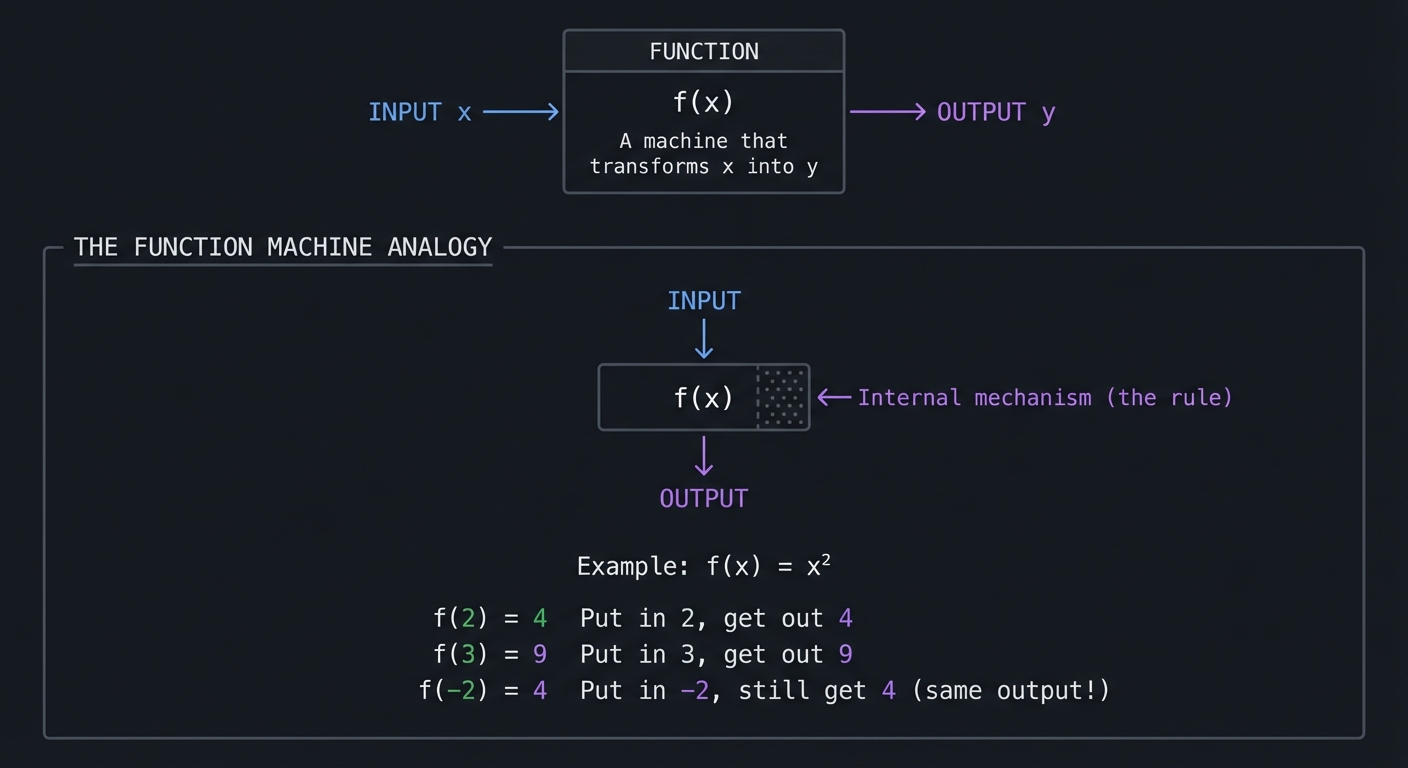
A function is a rule that takes an input and produces exactly one output. This is the most important concept for ML because every ML model is a function.
                    ┌─────────────────────┐
                    │                     │
    INPUT ────────▶ │      FUNCTION       │ ────────▶ OUTPUT
      x             │       f(x)          │             y
                    │                     │
                    │  "A machine that    │
                    │   transforms x      │
                    │   into y"           │
                    └─────────────────────┘

┌────────────────────────────────────────────────────────────────────────┐
│                                                                        │
│  THE FUNCTION MACHINE ANALOGY                                          │
│  ═══════════════════════════                                           │
│                                                                        │
│           INPUT                                                        │
│             │                                                          │
│             ▼                                                          │
│      ┌──────────────┐                                                  │
│      │   ░░░░░░░░   │  ◄── Internal mechanism (the rule)               │
│      │   ░ f(x) ░   │                                                  │
│      │   ░░░░░░░░   │                                                  │
│      └──────────────┘                                                  │
│             │                                                          │
│             ▼                                                          │
│          OUTPUT                                                        │
│                                                                        │
│  Example: f(x) = x²                                                    │
│                                                                        │
│      f(2) = 4       "Put in 2, get out 4"                              │
│      f(3) = 9       "Put in 3, get out 9"                              │
│      f(-2) = 4      "Put in -2, still get 4" (same output!)            │
│                                                                        │
└────────────────────────────────────────────────────────────────────────┘
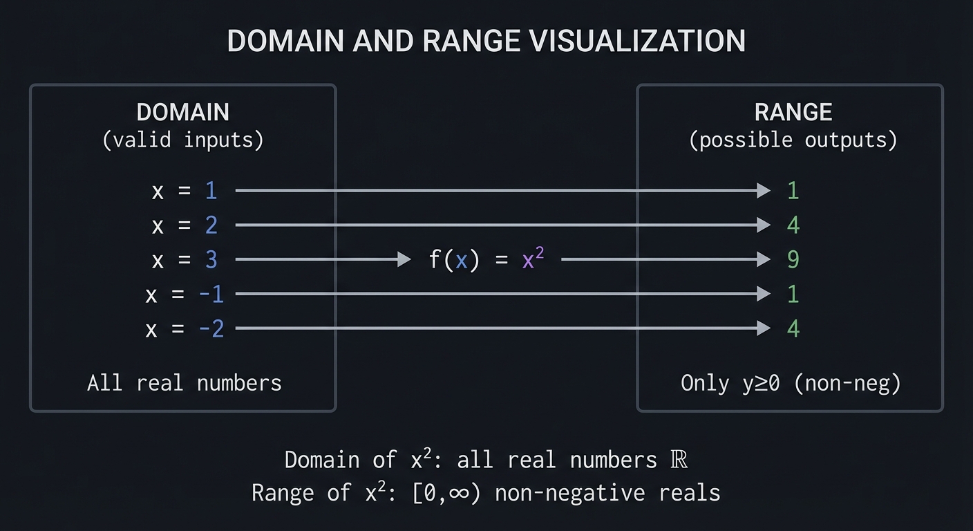
Domain and Range: What Goes In, What Comes Out
DOMAIN AND RANGE VISUALIZATION

         DOMAIN                                    RANGE
    (valid inputs)                            (possible outputs)

    ┌───────────┐                             ┌───────────┐
    │           │                             │           │
    │  x = 1  ──┼──────── f(x) = x² ─────────▶│── 1       │
    │  x = 2  ──┼──────────────────── ───────▶│── 4       │
    │  x = 3  ──┼────────────────────────────▶│── 9       │
    │  x = -1 ──┼────────────────────────────▶│── 1       │
    │  x = -2 ──┼────────────────────────────▶│── 4       │
    │           │                             │           │
    │  All real │                             │  Only y≥0 │
    │  numbers  │                             │  (non-neg)│
    └───────────┘                             └───────────┘

    Domain of x²: all real numbers ℝ
    Range of x²: [0, ∞) non-negative reals
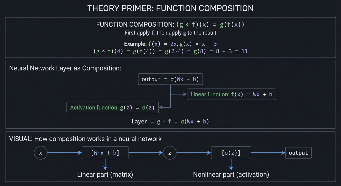
Function Composition: Combining Functions
Machine learning models are compositions of many functions. A neural network layer applies a linear function followed by a non-linear activation:
FUNCTION COMPOSITION: (g ∘ f)(x) = g(f(x))

"First apply f, then apply g to the result"

Example: f(x) = 2x, g(x) = x + 3

    (g ∘ f)(4) = g(f(4))
               = g(2·4)
               = g(8)
               = 8 + 3
               = 11

Neural Network Layer as Composition:
────────────────────────────────────

    output = σ(Wx + b)
             │ └──┬──┘
             │    │
             │    └── Linear function: f(x) = Wx + b
             │
             └─────── Activation function: g(z) = σ(z)

    Layer = g ∘ f = σ(Wx + b)

VISUAL: How composition works in a neural network

    x ──▶ [W·x + b] ──▶ z ──▶ [σ(z)] ──▶ output
          └───┬───┘          └──┬──┘
              │                 │
         Linear part      Nonlinear part
          (matrix)        (activation)
Reference: “Math for Programmers” by Paul Orland, Chapter 3, covers functions from a visual, computational perspective.
\1
Exponents and logarithms are inverse operations that appear throughout ML—in activation functions, loss functions, learning rate schedules, and information theory.
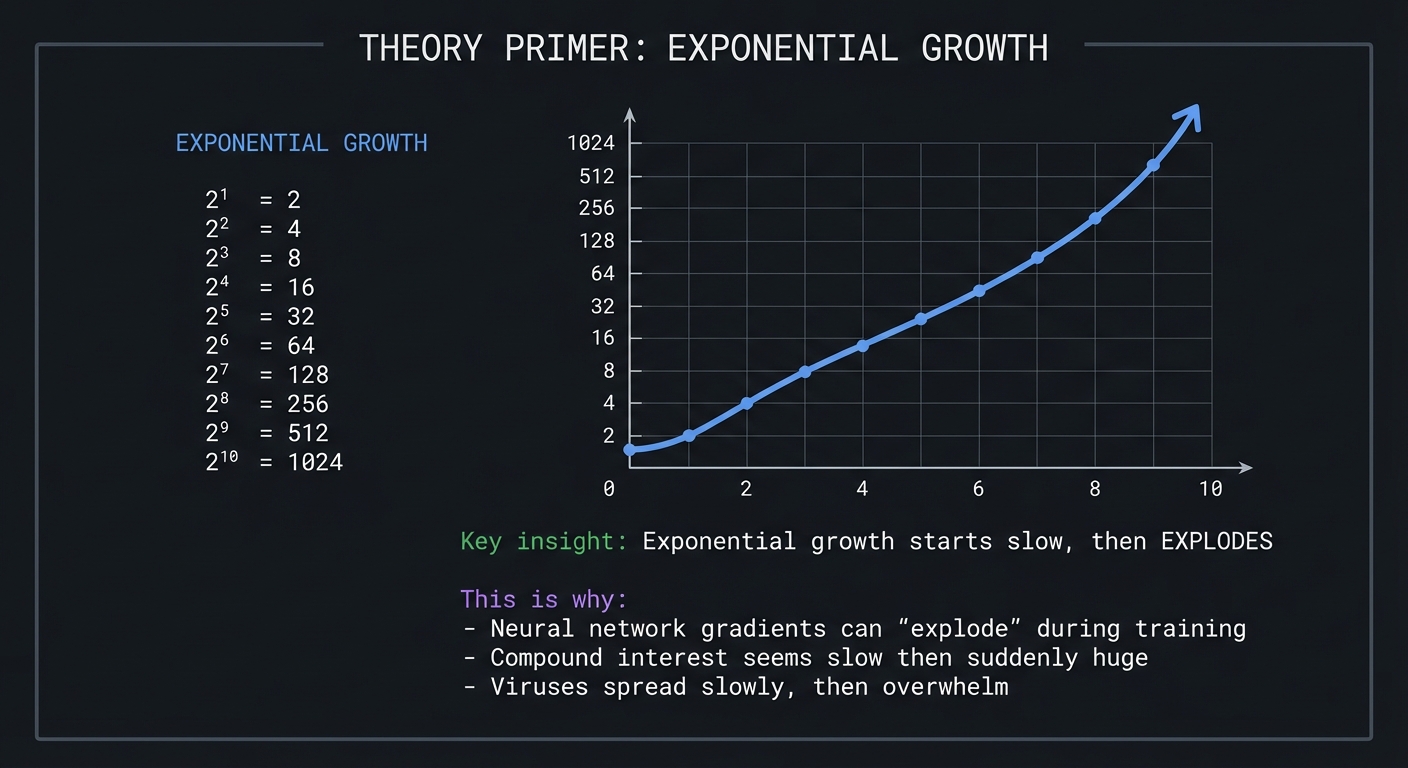
Exponential Growth: The Power of Repeated Multiplication
EXPONENTIAL GROWTH

    2¹ = 2
    2² = 4
    2³ = 8
    2⁴ = 16
    2⁵ = 32
    2⁶ = 64
    2⁷ = 128
    2⁸ = 256
    2⁹ = 512
    2¹⁰ = 1024

              │
         1024 ┼                                           ╭
              │                                          ╱
              │                                         ╱
          512 ┼                                        ╱
              │                                       ╱
          256 ┼                                     ╱
              │                                   ╱
          128 ┼                                 ╱
              │                              ╱
           64 ┼                           ╱
           32 ┼                       ╱╱
           16 ┼                  ╱╱╱
            8 ┼             ╱╱╱
            4 ┼        ╱╱╱
            2 ┼   ╱╱╱
              └───────────────────────────────────────────────
              0    2    4    6    8   10

    Key insight: Exponential growth starts slow, then EXPLODES

    This is why:
    - Neural network gradients can "explode" during training
    - Compound interest seems slow then suddenly huge
    - Viruses spread slowly, then overwhelm
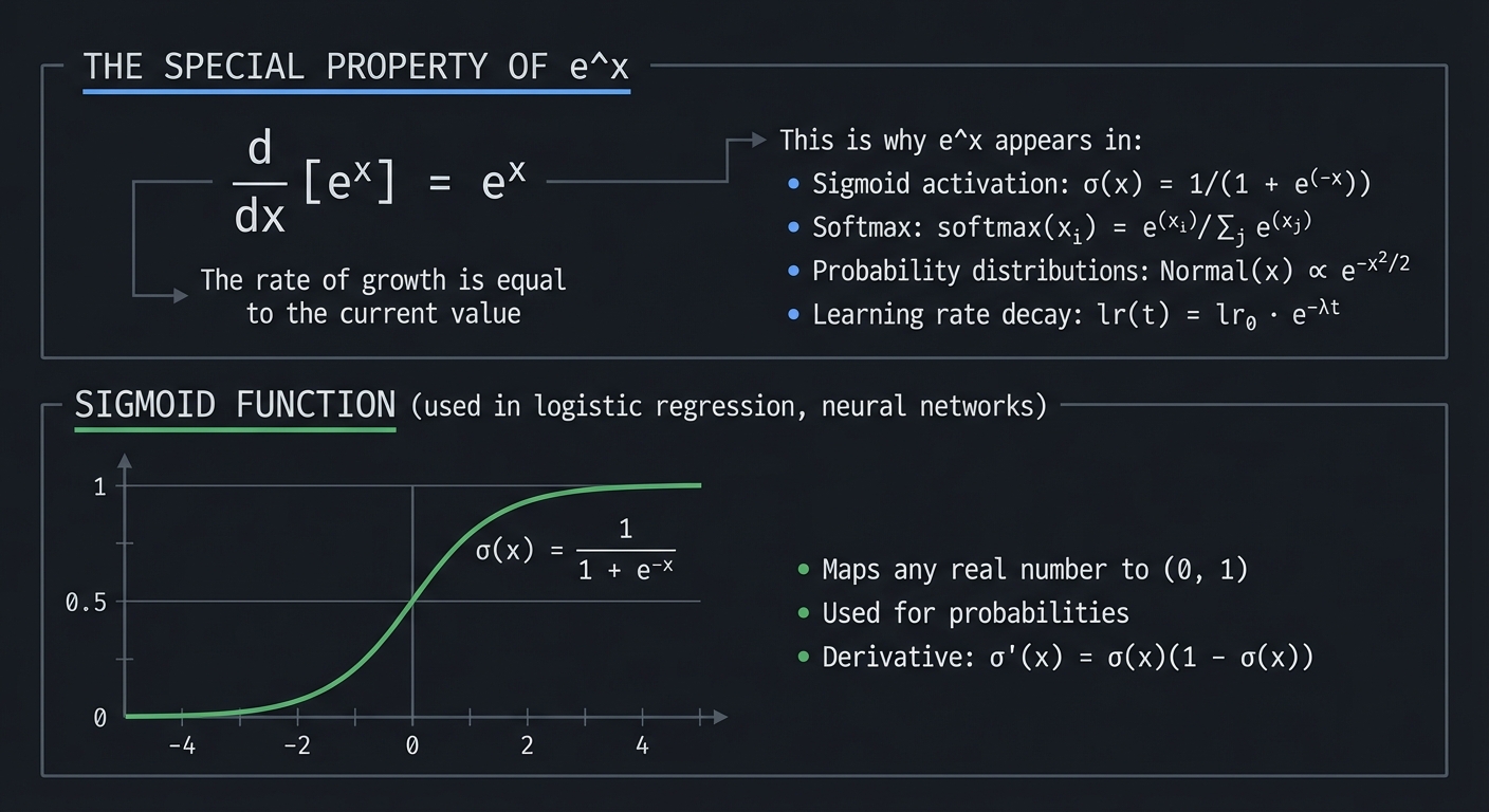
The Natural Exponential: e^x
The number e ≈ 2.71828… is special because the derivative of eˣ is itself:
THE SPECIAL PROPERTY OF e^x

    d/dx [eˣ] = eˣ

    "The rate of growth is equal to the current value"

This is why e^x appears in:
    - Sigmoid activation: σ(x) = 1/(1 + e^(-x))
    - Softmax: softmax(xᵢ) = e^(xᵢ) / Σⱼ e^(xⱼ)
    - Probability distributions: Normal(x) ∝ e^(-x²/2)
    - Learning rate decay: lr(t) = lr₀ · e^(-λt)

SIGMOID FUNCTION (used in logistic regression, neural networks)

         1   ┼─────────────────────────────────────────
             │                           ╭───────────
             │                        ╱╱╱
         0.5 ┼────────────────────╱╱╱───────────────
             │               ╱╱╱
             │          ╱╱╱╱
         0   ┼────╱╱╱──────────────────────────────────
             └──────┼───────┼───────┼───────┼──────────
                   -4      -2       0       2       4

    σ(x) = 1 / (1 + e^(-x))

    - Maps any real number to (0, 1)
    - Used for probabilities
    - Derivative: σ'(x) = σ(x)(1 - σ(x))
Logarithms: The Inverse of Exponentiation
LOGARITHMS AS INVERSE OPERATIONS

    Exponential:    2³ = 8
    Logarithmic:    log₂(8) = 3

    "2 to the power of WHAT equals 8?"
    Answer: 3

THE RELATIONSHIP:

    If b^y = x, then log_b(x) = y

    b^(log_b(x)) = x     (they undo each other)
    log_b(b^x) = x       (they undo each other)

COMMON LOGARITHMS IN ML:

    log₂(x)   - Base 2, used in information theory (bits)
    log₁₀(x)  - Base 10, used for order of magnitude
    ln(x)     - Natural log (base e), used in calculus/ML

    ln(e) = 1
    ln(1) = 0
    ln(0) = -∞  (undefined, approaches negative infinity)
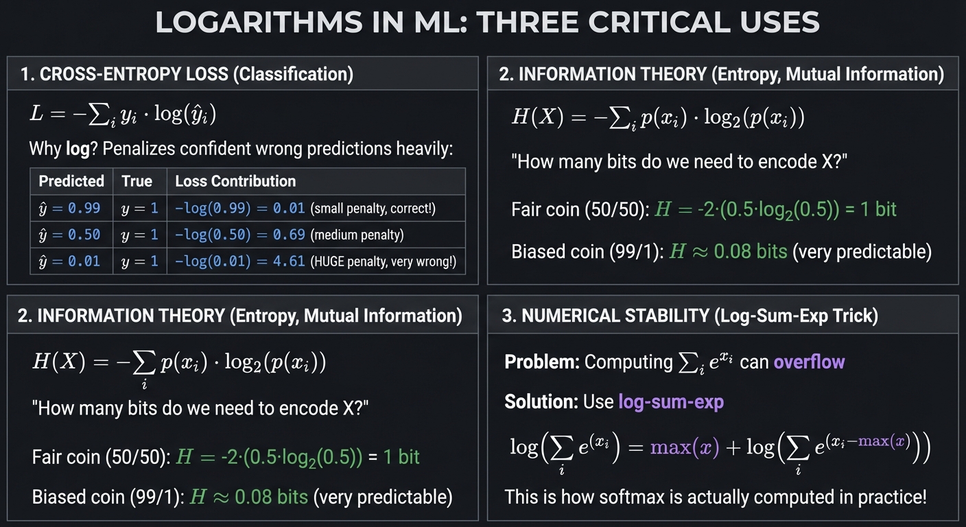
Why Logarithms Appear in Machine Learning
LOGARITHMS IN ML: THREE CRITICAL USES

1. CROSS-ENTROPY LOSS (Classification)
───────────────────────────────────────
    L = -Σᵢ yᵢ · log(ŷᵢ)

    Why log? Penalizes confident wrong predictions heavily:

    Predicted   True    Loss Contribution
    ─────────────────────────────────────
    ŷ = 0.99    y = 1   -log(0.99) = 0.01  (small penalty, correct!)
    ŷ = 0.50    y = 1   -log(0.50) = 0.69  (medium penalty)
    ŷ = 0.01    y = 1   -log(0.01) = 4.61  (HUGE penalty, very wrong!)


2. INFORMATION THEORY (Entropy, Mutual Information)
────────────────────────────────────────────────────
    H(X) = -Σᵢ p(xᵢ) · log₂(p(xᵢ))

    "How many bits do we need to encode X?"

    Fair coin (50/50): H = -2·(0.5·log₂(0.5)) = 1 bit
    Biased coin (99/1): H ≈ 0.08 bits (very predictable)


3. NUMERICAL STABILITY (Log-Sum-Exp Trick)
───────────────────────────────────────────
    Problem: Computing Σᵢ e^(xᵢ) can overflow

    Solution: Use log-sum-exp

    log(Σᵢ e^(xᵢ)) = max(x) + log(Σᵢ e^(xᵢ - max(x)))

    This is how softmax is actually computed in practice!
Reference: “C Programming: A Modern Approach” by K. N. King, Chapter 7, covers the numerical representation of these values, while “Math for Programmers” Chapter 2 provides the mathematical intuition.
\1
Trigonometry connects angles to ratios, circles to waves, and appears in ML through signal processing, attention mechanisms, and positional encodings.
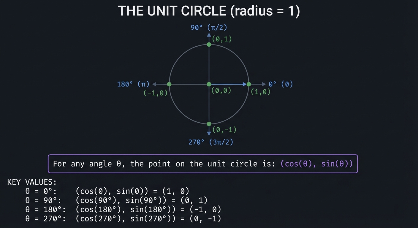
The Unit Circle: Where It All Begins
THE UNIT CIRCLE (radius = 1)

                        90° (π/2)
                           │
                    (0,1)  │
                      ╱╲   │
                     ╱  ╲  │
                    ╱    ╲ │
                   ╱      ╲│
    180° (π) ─────●────────●────────● 0° (0)
              (-1,0)       │(0,0)  (1,0)
                          ╲│╱
                           │
                           │
                        (0,-1)
                        270° (3π/2)

For any angle θ, the point on the unit circle is:
    (cos(θ), sin(θ))

KEY VALUES:
    θ = 0°:    (cos(0), sin(0)) = (1, 0)
    θ = 90°:   (cos(90°), sin(90°)) = (0, 1)
    θ = 180°:  (cos(180°), sin(180°)) = (-1, 0)
    θ = 270°:  (cos(270°), sin(270°)) = (0, -1)
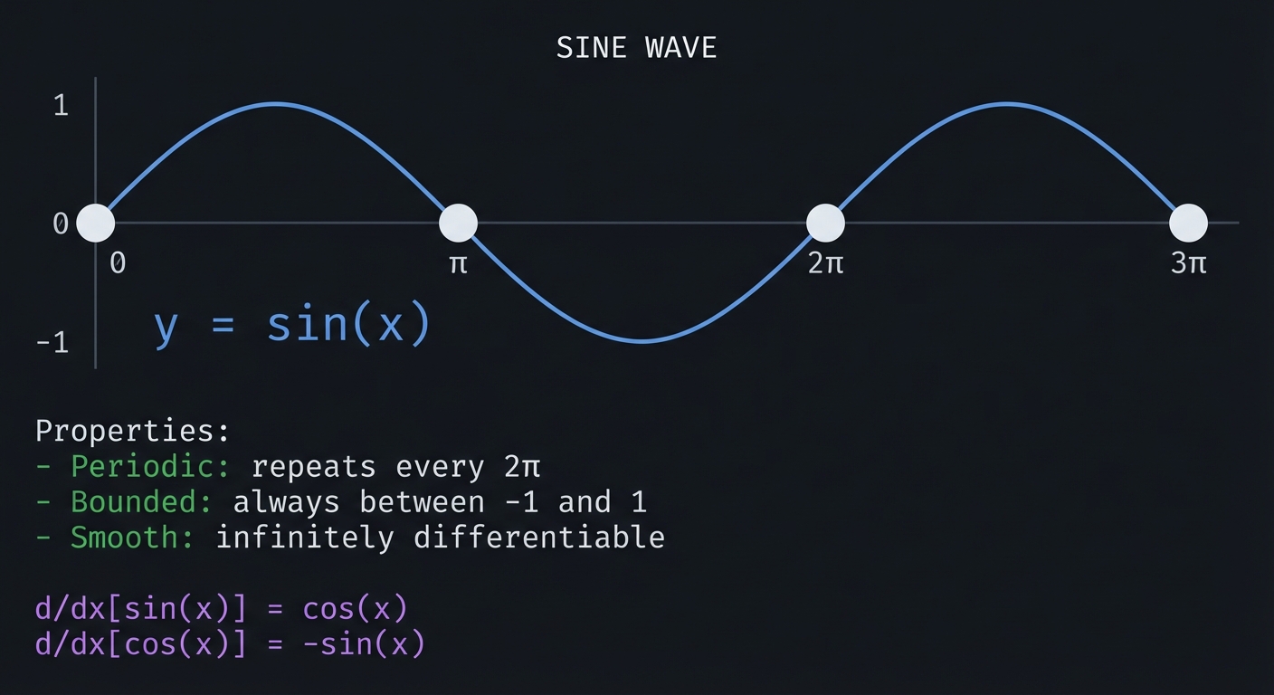
Sine and Cosine as Waves
SINE WAVE

    1 ┼           ╭───╮               ╭───╮
      │          ╱     ╲             ╱     ╲
      │         ╱       ╲           ╱       ╲
    0 ┼────────●─────────●─────────●─────────●────
      │       0          π         2π         3π
      │         ╲       ╱           ╲       ╱
      │          ╲     ╱             ╲     ╱
   -1 ┼           ╰───╯               ╰───╯

    y = sin(x)

    Properties:
    - Periodic: repeats every 2π
    - Bounded: always between -1 and 1
    - Smooth: infinitely differentiable

    d/dx[sin(x)] = cos(x)
    d/dx[cos(x)] = -sin(x)
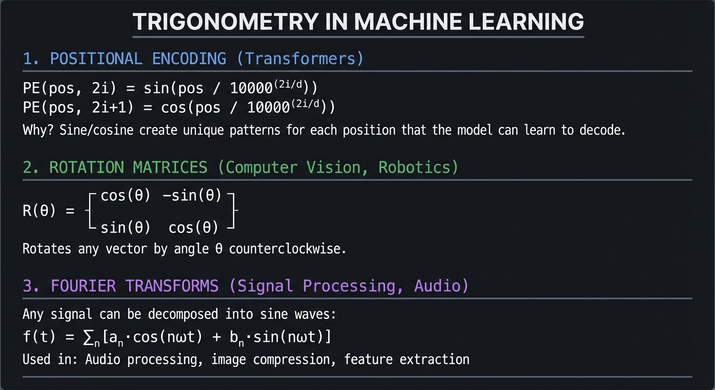
Why Trigonometry Matters for ML
TRIGONOMETRY IN MACHINE LEARNING

1. POSITIONAL ENCODING (Transformers)
─────────────────────────────────────
    PE(pos, 2i) = sin(pos / 10000^(2i/d))
    PE(pos, 2i+1) = cos(pos / 10000^(2i/d))

    Why? Sine/cosine create unique patterns for each position
    that the model can learn to decode.


2. ROTATION MATRICES (Computer Vision, Robotics)
────────────────────────────────────────────────
    R(θ) = ┌ cos(θ)  -sin(θ) ┐
           │                 │
           └ sin(θ)   cos(θ) ┘

    Rotates any vector by angle θ counterclockwise.


3. FOURIER TRANSFORMS (Signal Processing, Audio)
────────────────────────────────────────────────
    Any signal can be decomposed into sine waves:

    f(t) = Σₙ [aₙ·cos(nωt) + bₙ·sin(nωt)]

    Used in: Audio processing, image compression, feature extraction
Reference: “Computer Graphics from Scratch” by Gabriel Gambetta covers trigonometry in the context of rotations and projections.
\1
Linear algebra is not optional for ML—it IS the implementation. Every neural network forward pass is matrix multiplication. Every weight update is vector arithmetic. Every dataset is a matrix.
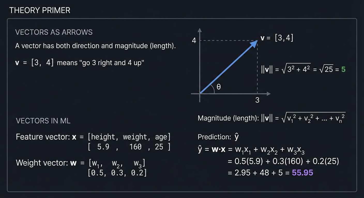
Vectors: Direction and Magnitude
VECTORS AS ARROWS

    A vector has both direction and magnitude (length).

    v = [3, 4]  means "go 3 right and 4 up"

        4 │        ↗ v = [3,4]
          │       ╱
          │      ╱
          │     ╱   ||v|| = √(3² + 4²) = √25 = 5
          │    ╱
          │   ╱
          │  ╱
          │ ╱
          │╱θ
          └────────────────────
                   3

    Magnitude (length):  ||v|| = √(v₁² + v₂² + ... + vₙ²)

VECTORS IN ML:

    Feature vector: x = [height, weight, age]
                        [  5.9,    160,  25 ]

    Weight vector:  w = [w₁, w₂, w₃]
                        [0.5, 0.3, 0.2]

    Prediction:     ŷ = w·x = w₁x₁ + w₂x₂ + w₃x₃
                        = 0.5(5.9) + 0.3(160) + 0.2(25)
                        = 2.95 + 48 + 5 = 55.95
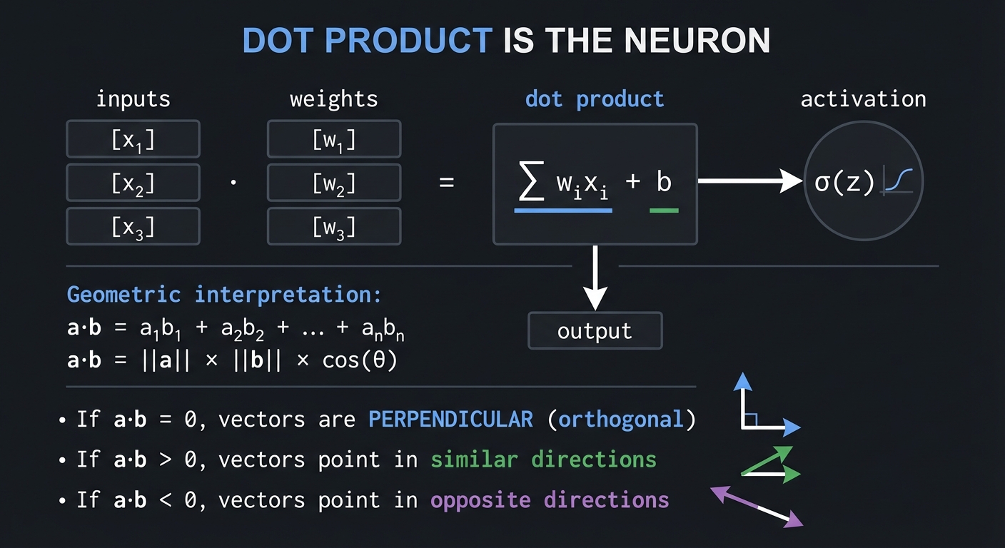
The Dot Product: The Neuron
DOT PRODUCT IS THE NEURON:

    inputs     weights       dot product      activation
    [x₁]   ·   [w₁]    =    Σ wᵢxᵢ + b   →     σ(z)
    [x₂]       [w₂]            │
    [x₃]       [w₃]            ▼
                              output

    a·b = a₁b₁ + a₂b₂ + ... + aₙbₙ

    Geometric interpretation:
    a·b = ||a|| × ||b|| × cos(θ)

    If a·b = 0, vectors are PERPENDICULAR (orthogonal)
    If a·b > 0, vectors point in similar directions
    If a·b < 0, vectors point in opposite directions
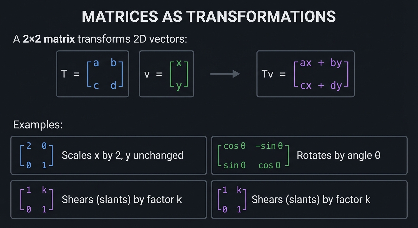
Matrices as Transformations
MATRICES AS TRANSFORMATIONS

    A 2×2 matrix transforms 2D vectors:

    T = ┌ a  b ┐     v = ┌ x ┐
        │      │         │   │
        └ c  d ┘         └ y ┘

    Tv = ┌ ax + by ┐
         │         │
         └ cx + dy ┘

    Examples:

    ┌ 2  0 ┐  Scales x by 2, y unchanged
    │      │
    └ 0  1 ┘

    ┌ cos θ  -sin θ ┐  Rotates by angle θ
    │               │
    └ sin θ   cos θ ┘

    ┌ 1  k ┐  Shears (slants) by factor k
    │      │
    └ 0  1 ┘
Eigenvalues and Eigenvectors: The Key ML Concept
EIGENVECTORS: SPECIAL DIRECTIONS

    For a matrix A, an eigenvector v satisfies:

        A·v = λ·v

    "When A transforms v, v doesn't change direction,
     only scales by factor λ (the eigenvalue)"

WHY EIGENVECTORS MATTER FOR ML:

1. PCA: Eigenvectors of covariance matrix = principal components
        (directions of maximum variance in data)

2. PageRank: The ranking vector is the dominant eigenvector
             of the link matrix

3. Spectral Clustering: Uses eigenvectors of similarity matrix

4. Stability: Eigenvalues tell if gradients will explode/vanish
              |λ| > 1: grows exponentially (exploding gradients)
              |λ| < 1: shrinks exponentially (vanishing gradients)
Reference: “Math for Programmers” by Paul Orland, Chapters 5-7, covers vectors and matrices with visual intuition. “Linear Algebra Done Right” by Sheldon Axler provides deeper theoretical foundations.
\1
Calculus answers the question: “How does the output change when I change the input?” This is fundamental to ML because training is about adjusting parameters to change (reduce) the loss.
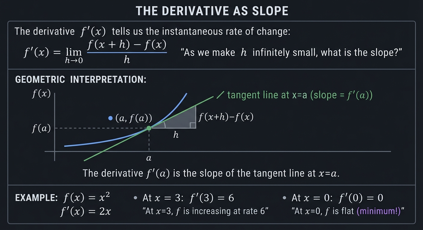
Derivatives: Rate of Change
THE DERIVATIVE AS SLOPE

    The derivative f'(x) tells us the instantaneous rate of change:

        f'(x) = lim    f(x + h) - f(x)
               h→0    ─────────────────
                            h

    "As we make h infinitely small, what is the slope?"

GEOMETRIC INTERPRETATION:

    f(x)
      │             ╱ tangent line at x=a
      │           ╱   (slope = f'(a))
      │          ╱
      │        ●─────────────
      │      ╱╱│
      │    ╱╱  │
      │  ╱╱    │ f(a)
      │╱╱──────┼─────────────────
              a

    The derivative f'(a) is the slope of the tangent line at x=a.

EXAMPLE: f(x) = x²

    f'(x) = 2x

    At x = 3: f'(3) = 6
        "At x=3, f is increasing at rate 6"

    At x = 0: f'(0) = 0
        "At x=0, f is flat (minimum!)"
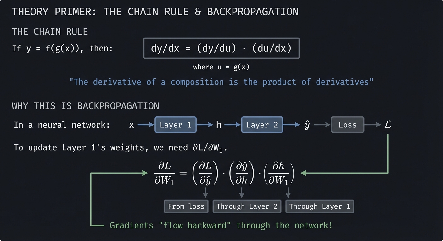
The Chain Rule: The Heart of Backpropagation
THE CHAIN RULE

    If y = f(g(x)), then:

        dy/dx = (dy/du) · (du/dx)

    where u = g(x)

    "The derivative of a composition is the product of derivatives"

WHY THIS IS BACKPROPAGATION:

    In a neural network:

    x → [Layer 1] → h → [Layer 2] → ŷ → [Loss] → L

    To update Layer 1's weights, we need ∂L/∂W₁.

    Chain rule:
    ∂L/∂W₁ = (∂L/∂ŷ) · (∂ŷ/∂h) · (∂h/∂W₁)
             └──┬──┘   └──┬──┘   └──┬──┘
                │         │         │
           From loss  Through  Through
                      Layer 2  Layer 1

    Gradients "flow backward" through the network!
Gradients: Derivatives in Multiple Dimensions
THE GRADIENT

    The gradient ∇f collects all partial derivatives into a vector:

        ∇f = [∂f/∂x, ∂f/∂y, ∂f/∂z, ...]

    For f(x, y) = x² + y²:

        ∇f = [2x, 2y]

        At point (3, 4): ∇f = [6, 8]

    CRITICAL PROPERTY:
    The gradient points in the direction of STEEPEST ASCENT.

    Therefore, to minimize f, we move in direction -∇f (steepest descent).
Reference: “Calculus” by James Stewart provides comprehensive coverage. “Neural Networks and Deep Learning” by Michael Nielsen explains backpropagation beautifully.
\1
ML models don’t just make predictions—they reason about uncertainty. Probability provides the framework for this reasoning.
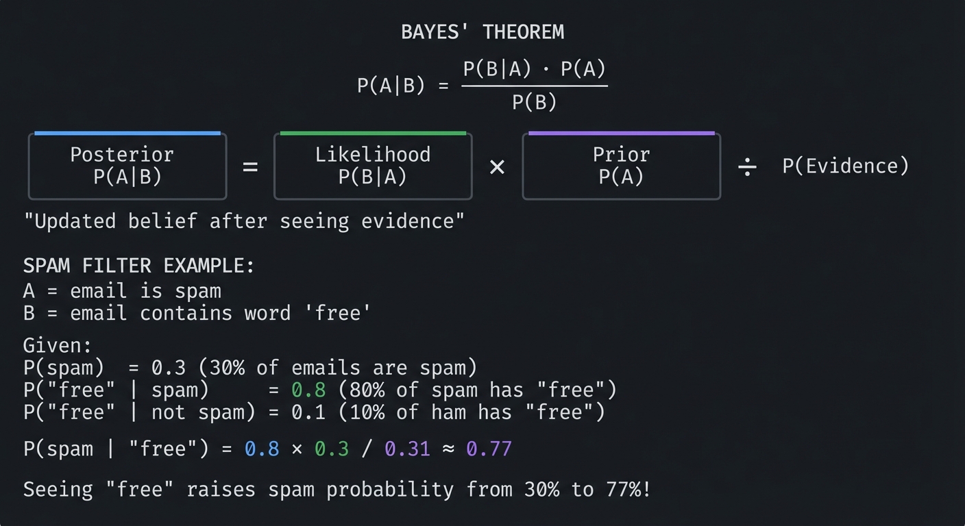
Bayes’ Theorem: Updating Beliefs
BAYES' THEOREM

    P(A|B) = P(B|A) · P(A)
             ─────────────
                P(B)

    ┌─────────┐   ┌─────────┐   ┌─────────┐
    │Posterior│ = │Likelihood│ × │  Prior  │  ÷  P(Evidence)
    │ P(A|B)  │   │  P(B|A) │   │  P(A)   │
    └─────────┘   └─────────┘   └─────────┘

    "Updated belief after seeing evidence"

SPAM FILTER EXAMPLE:

    A = email is spam
    B = email contains word "free"

    Given:
        P(spam) = 0.3                    (30% of emails are spam)
        P("free" | spam) = 0.8           (80% of spam has "free")
        P("free" | not spam) = 0.1       (10% of ham has "free")

    P(spam | "free") = 0.8 × 0.3 / 0.31 ≈ 0.77

    Seeing "free" raises spam probability from 30% to 77%!
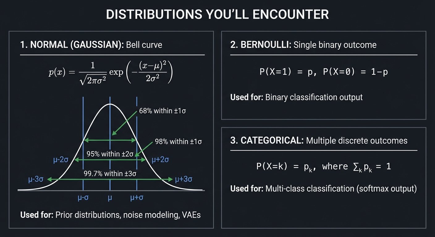
Key Distributions for ML
DISTRIBUTIONS YOU'LL ENCOUNTER

1. NORMAL (GAUSSIAN): Bell curve
   ────────────────────────────────
   p(x) = (1/√(2πσ²)) exp(-(x-μ)²/(2σ²))

         │     ╭───╮
         │    ╱     ╲     68% within ±1σ
         │   ╱       ╲    95% within ±2σ
         │  ╱         ╲   99.7% within ±3σ
         │ ╱           ╲
         └───────────────────
              μ-σ  μ  μ+σ

   Used for: Prior distributions, noise modeling, VAEs


2. BERNOULLI: Single binary outcome
   ────────────────────────────────
   P(X=1) = p, P(X=0) = 1-p

   Used for: Binary classification output


3. CATEGORICAL: Multiple discrete outcomes
   ─────────────────────────────────────────
   P(X=k) = pₖ, where Σₖ pₖ = 1

   Used for: Multi-class classification (softmax output)
Reference: “Think Bayes” by Allen Downey provides an intuitive, computational approach to probability.
\1
All of machine learning reduces to optimization: define a loss function that measures how wrong your model is, then find parameters that minimize it.
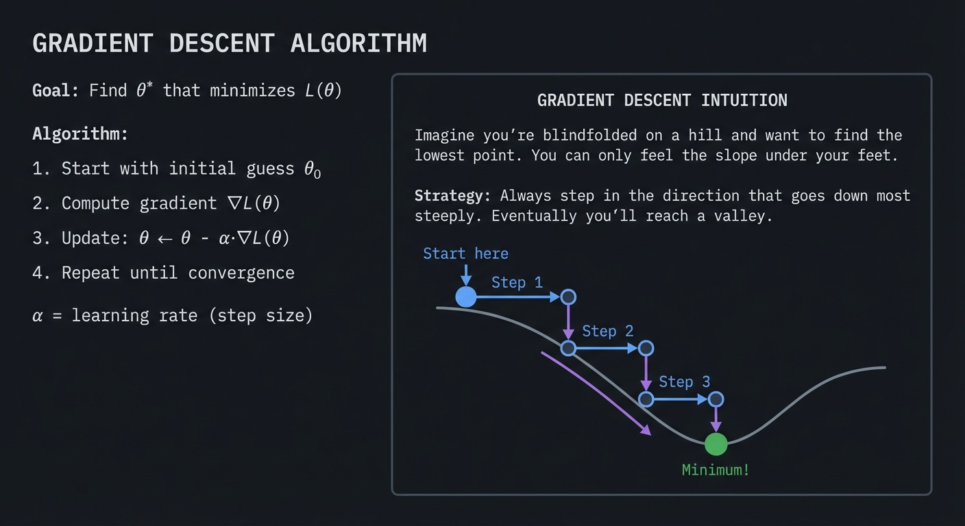
Gradient Descent: Walking Downhill
GRADIENT DESCENT ALGORITHM

    Goal: Find θ* that minimizes L(θ)

    Algorithm:
    1. Start with initial guess θ₀
    2. Compute gradient ∇L(θ)
    3. Update: θ ← θ - α·∇L(θ)
    4. Repeat until convergence

    α = learning rate (step size)

    ┌─────────────────────────────────────────────────────────────┐
    │                                                             │
    │   GRADIENT DESCENT INTUITION                                │
    │                                                             │
    │   Imagine you're blindfolded on a hill and want to find     │
    │   the lowest point. You can only feel the slope under       │
    │   your feet.                                                │
    │                                                             │
    │   Strategy: Always step in the direction that goes down     │
    │   most steeply. Eventually you'll reach a valley.           │
    │                                                             │
    │        Start here                                           │
    │            ↓                                                │
    │          ●───→ Step 1                                       │
    │              ╲                                              │
    │               ●───→ Step 2                                  │
    │                   ╲                                         │
    │                    ●───→ Step 3                             │
    │                        ╲                                    │
    │                         ● Minimum!                          │
    │                                                             │
    └─────────────────────────────────────────────────────────────┘
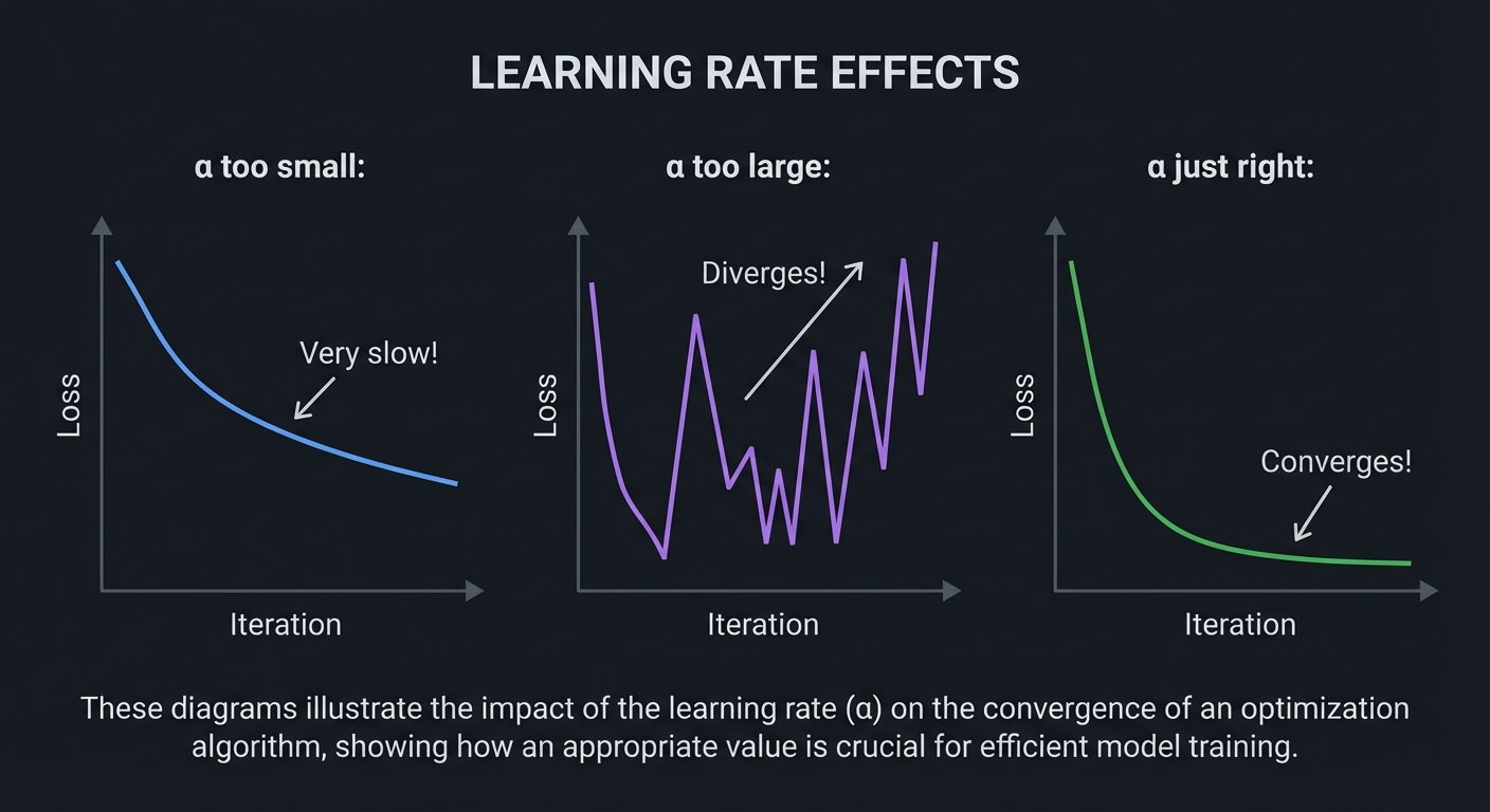
Learning Rate Effects
LEARNING RATE EFFECTS

    α too small:                α too large:

    Loss                        Loss
      │                           │    ╱╲    ╱╲
      │╲                          │   ╱  ╲  ╱  ╲
      │ ╲                         │  ╱    ╲╱    ╲
      │  ╲                        │ ╱            ↗ Diverges!
      │   ╲                       │╱
      │    ╲                      └────────────────
      │     ╲                         Iteration
      │      ╲
      │       ╲    Very slow!
      └────────╲─────────────
                Iteration


    α just right:

    Loss
      │╲
      │ ╲
      │  ╲
      │   ╲
      │    ╲
      │     ╲_______________  Converges!
      └──────────────────────
          Iteration
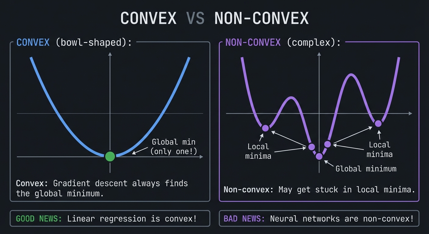
Convexity: When Optimization is Easy
CONVEX VS NON-CONVEX

    CONVEX (bowl-shaped):          NON-CONVEX (complex):

         ╲     ╱                        ╱╲   ╱╲
          ╲   ╱                        ╱  ╲ ╱  ╲
           ╲ ╱                        ╱    ●    ╲
            ●                        ●           ●
       Global min                  Local      Local
    (only one!)                   minima      minima

    Convex: Gradient descent always finds the global minimum.
    Non-convex: May get stuck in local minima.

GOOD NEWS: Linear regression is convex!
BAD NEWS: Neural networks are non-convex!
Reference: “Hands-On Machine Learning” by Aurelien Geron, Chapter 4, provides practical coverage of gradient descent. “Deep Learning” by Goodfellow, Bengio, and Courville gives theoretical depth.
\1
COMPLETE MATHEMATICAL FLOW OF TRAINING

INPUT: x ∈ ℝⁿ (feature vector)
TARGET: y ∈ ℝ (true label)
PARAMETERS: W₁, b₁, W₂, b₂ (weight matrices and bias vectors)

═══════════════════════════════════════════════════════════════════

FORWARD PASS (Linear Algebra + Functions)
──────────────────────────────────────────

Layer 1:
    z₁ = W₁ · x + b₁         ← Matrix multiplication (linear algebra)
    a₁ = σ(z₁)               ← Activation function (functions)

Layer 2 (output):
    z₂ = W₂ · a₁ + b₂        ← Matrix multiplication
    ŷ = σ(z₂)                ← Sigmoid for probability (exp/log)

═══════════════════════════════════════════════════════════════════

LOSS COMPUTATION (Probability)
───────────────────────────────

    L = -[y·log(ŷ) + (1-y)·log(1-ŷ)]    ← Cross-entropy (probability)

═══════════════════════════════════════════════════════════════════

BACKWARD PASS (Calculus - Chain Rule)
──────────────────────────────────────

Output layer gradient:
    ∂L/∂z₂ = ŷ - y           ← Derivative of loss + sigmoid
    ∂L/∂W₂ = a₁ᵀ · ∂L/∂z₂    ← Chain rule
    ∂L/∂b₂ = ∂L/∂z₂

Hidden layer gradient (chain rule through):
    ∂L/∂a₁ = W₂ᵀ · ∂L/∂z₂    ← Gradient flows backward
    ∂L/∂z₁ = ∂L/∂a₁ ⊙ σ'(z₁) ← Element-wise with activation derivative
    ∂L/∂W₁ = xᵀ · ∂L/∂z₁     ← Chain rule
    ∂L/∂b₁ = ∂L/∂z₁

═══════════════════════════════════════════════════════════════════

PARAMETER UPDATE (Optimization)
─────────────────────────────────

    W₁ ← W₁ - α · ∂L/∂W₁     ← Gradient descent
    b₁ ← b₁ - α · ∂L/∂b₁
    W₂ ← W₂ - α · ∂L/∂W₂
    b₂ ← b₂ - α · ∂L/∂b₂

═══════════════════════════════════════════════════════════════════

REPEAT for each batch until loss converges!
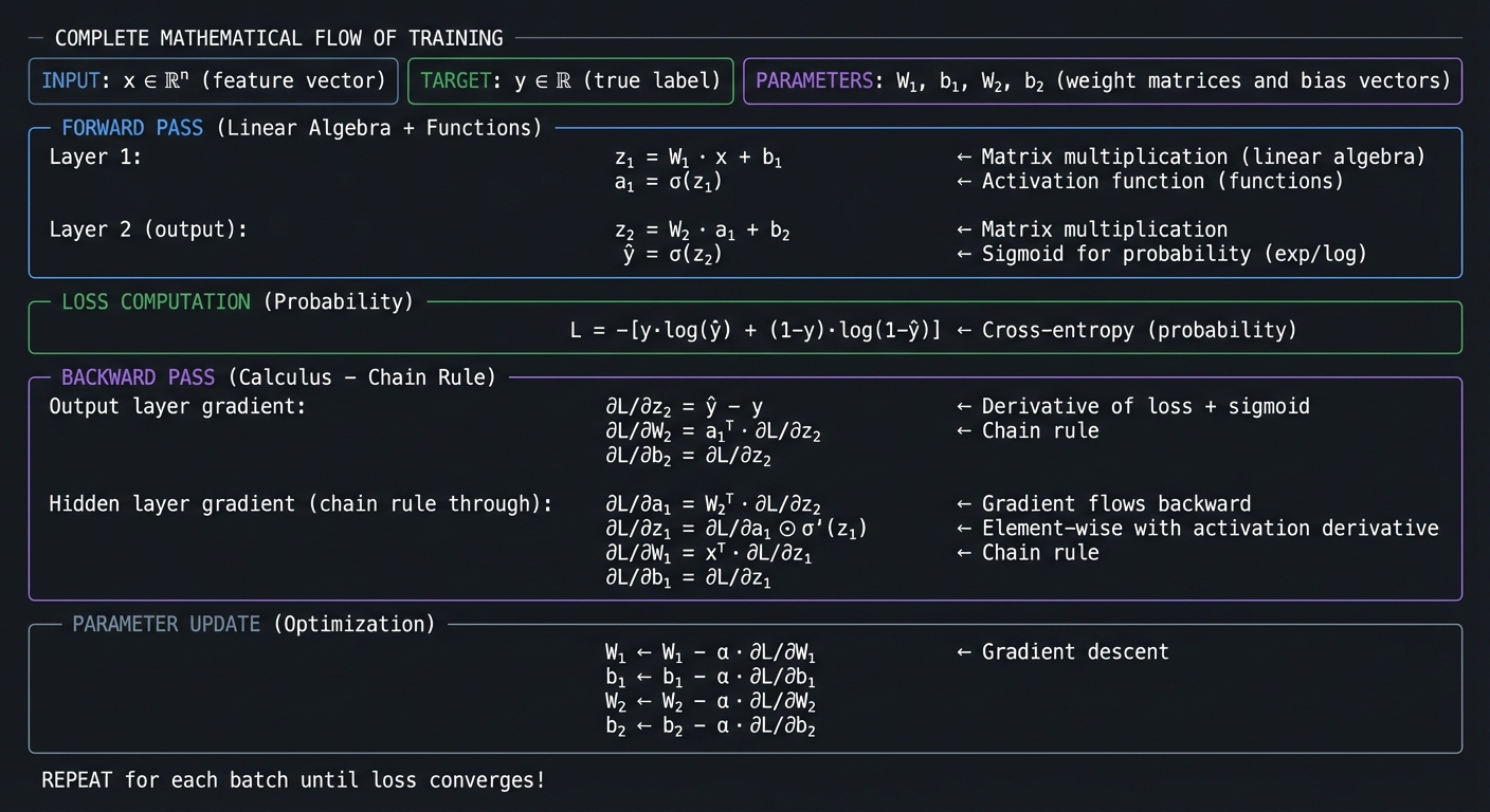
This is what happens inside model.fit(). Every concept we’ve covered—algebra, functions, exponents, linear algebra, calculus, probability, and optimization—comes together in this elegant mathematical dance.
When you complete these 31 projects, you won’t just understand this diagram—you’ll have built every component yourself.
Glossary
- Feature: A measurable input variable used by a model to make predictions.
- Parameter: A learnable value (for example, a weight or bias) updated during training.
- Loss Function: A numeric score that measures prediction error; training minimizes this value.
- Gradient: Vector of partial derivatives indicating the direction of steepest increase in loss.
- Convexity: A shape property where any local minimum is also a global minimum.
- Overfitting: When a model memorizes training data patterns that do not generalize to new data.
- Regularization: A constraint added to reduce overfitting by penalizing complex models.
- Likelihood: Probability of observing the data under a chosen model and parameter set.
- Covariance: Measure of how two variables vary together around their means.
- Condition Number: A measure of how sensitive a numerical problem is to small input perturbations.
Why Math for Machine Learning Matters
Modern ML systems are not bottlenecked by model APIs; they are bottlenecked by data quality, objective design, numerical behavior, and evaluation rigor.
- In 2024, 78% of organizations reported using AI, up from 55% in 2023 (Stanford AI Index 2025).
- The same report notes inference-cost declines for GPT-3.5-class systems of more than 280x between November 2022 and October 2024, which increases pressure to ship faster but safely (Stanford AI Index 2025).
- U.S. labor demand is also strong: Data Scientist employment is projected to grow 36% from 2023 to 2033 (U.S. Bureau of Labor Statistics).
- Developer workflow impact is now mainstream: 84.6% of developers are using or planning to use AI tools (Stack Overflow Developer Survey 2025).
Old "Model-Centric" Loop                 New "Math + Systems" Loop
+-----------------------+                 +------------------------------+
| Pick model            |                 | Define objective + constraints|
| Train quickly         |                 | Validate assumptions          |
| Report single metric  |                 | Stress test numerics          |
| Ship                  |                 | Measure uncertainty + cost    |
+-----------------------+                 +------------------------------+
          |                                             |
          v                                             v
  High hidden failure risk                      Lower operational surprises
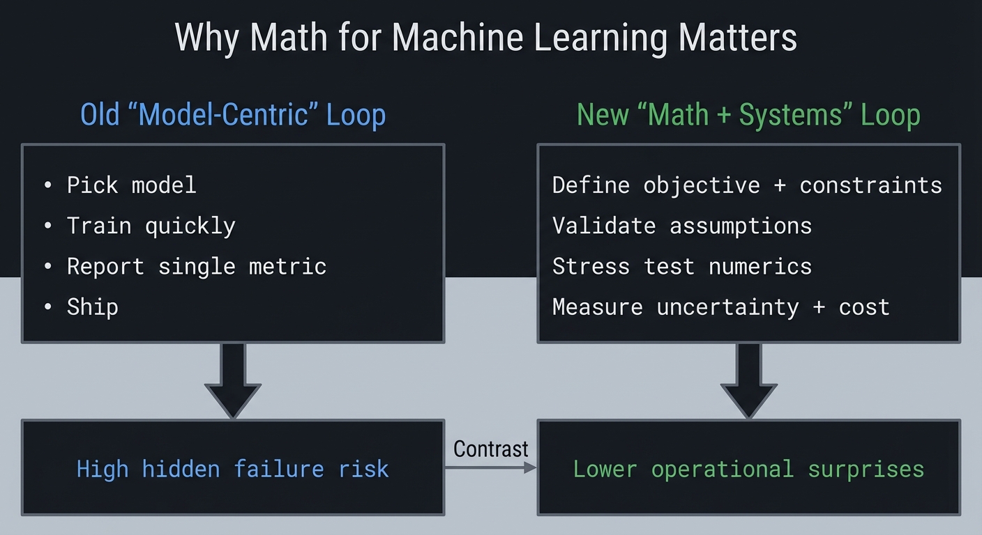
Context and evolution: early ML education emphasized algorithms and libraries; current practice increasingly emphasizes data/metric realism, failure analysis, and reproducibility discipline.
Concept Summary Table
| Concept Cluster | What You Need to Internalize | |||
|---|---|---|---|---|
| Arithmetic & Order of Operations | PEMDAS is not arbitrary - it reflects how mathematical expressions compose. Parentheses group, exponents bind tightest, multiplication/division before addition/subtraction. This hierarchy appears everywhere: in code parsing, in how neural networks process layer-by-layer, in how we decompose complex problems. | |||
| Variables & Algebraic Expressions | Variables are placeholders that let you express relationships abstractly. The power of algebra is generalization - once you solve ax + b = c for x, you’ve solved infinitely many specific problems. In ML, model parameters (weights) are variables we solve for. |
|||
| Equations & Solving Systems | An equation is a constraint that must be satisfied. Solving means finding values that satisfy all constraints simultaneously. Linear systems (Ax = b) are the foundation of regression. The key insight: transforming equations preserves solutions - you can manipulate freely as long as you apply operations to both sides. |
|||
| Functions (Domain, Range, Mapping) | Functions are deterministic input-output machines: each input maps to exactly one output. Domain = valid inputs, Range = possible outputs. ML models ARE functions: they take features as input and produce predictions as output. Understanding functions means understanding that f(x) is a recipe, not a number. |
|||
| Function Composition & Inverse | Composing functions (f(g(x))) chains transformations - this is exactly what neural network layers do. Inverse functions “undo” each other (f(f^{-1}(x)) = x). Log and exp are inverses. Understanding composition is essential for backpropagation - gradients flow backward through composed functions via the chain rule. |
|||
| Exponents & Exponential Functions | Exponents represent repeated multiplication: a^n means “multiply a by itself n times.” Exponential functions (e^x) grow explosively and appear everywhere: compound interest, population growth, neural network activations (softmax, sigmoid). The number e (2.718…) is special because d/dx(e^x) = e^x. |
|||
| Logarithms | Logarithms are inverse of exponentiation: log_b(x) = y means b^y = x. They convert multiplication to addition (log(ab) = log(a) + log(b)), making them invaluable for numerical stability. In ML: log-probabilities prevent underflow, cross-entropy loss uses logs, and we often work in log-space for numerical reasons. |
|||
| Trigonometry (Sine, Cosine, Unit Circle) | Trig functions encode circular relationships: given an angle, sin/cos return coordinates on the unit circle. They’re periodic (repeat every 2pi), which makes them useful for modeling cycles. In ML: positional encodings in transformers use sin/cos, rotation matrices use them, and Fourier transforms decompose signals into sines and cosines. | |||
| Vectors & Vector Spaces | Vectors are ordered lists of numbers that represent points or directions in space. They can be added and scaled. A vector space is the set of all vectors you can create through these operations. In ML, every data point is a vector (feature vector), every word is a vector (embedding), every image is a vector (flattened pixels). | |||
| Vector Operations (Dot Product, Norm) | The dot product a.b = sum(a_i * b_i) measures similarity and alignment between vectors. The norm ||a|| measures vector length. Dot products are everywhere in ML: computing weighted sums, measuring cosine similarity, the forward pass of neurons. The norm appears in regularization and normalization. |
|||
| Matrices & Matrix Operations | Matrices are 2D arrays of numbers that represent linear transformations. Matrix multiplication applies one transformation after another. In ML, weight matrices transform inputs, batch computations use matrices, and images are matrices. Understanding matrix multiplication as “row-column dot products” is essential. | |||
| Linear Transformations | A linear transformation preserves addition and scaling: T(a+b) = T(a) + T(b) and T(ca) = cT(a). Every matrix represents a linear transformation. Neural network layers (before activation) are linear transformations. Understanding this geometric view - matrices rotate, scale, shear, project - builds deep intuition. |
|||
| Gaussian Elimination & Solving Linear Systems | Gaussian elimination systematically solves Ax = b by reducing to row echelon form. It reveals whether solutions exist (consistency), how many (uniqueness vs infinite), and finds them. This is the foundation of understanding when linear systems have solutions - critical for regression and optimization. |
|||
| Determinants | The determinant measures how a matrix transformation scales volume. If det(A) = 0, the matrix squashes space to a lower dimension (singular/non-invertible). Non-zero determinant means the transformation is reversible. In ML, determinants appear in Gaussian distributions, change of variables, and checking matrix invertibility. | |||
| Matrix Inverse | The inverse A^{-1} “undoes” matrix A: A * A^{-1} = I. Only square matrices with non-zero determinant have inverses. The normal equation for linear regression uses matrix inverse: w = (X^T X)^{-1} X^T y. Understanding when inverses exist and how to compute them is fundamental. |
|||
| Eigenvalues & Eigenvectors | Eigenvectors are special directions that don’t change orientation under transformation - they only scale by the eigenvalue: Av = lambda*v. They reveal the “natural axes” of a transformation. In ML: PCA finds eigenvectors of covariance, PageRank is an eigenvector problem, stability analysis uses eigenvalues. This is arguably THE most important linear algebra concept for ML. |
|||
| Eigendecomposition & Diagonalization | When a matrix can be written as A = PDP^{-1} where D is diagonal, we’ve diagonalized it. The columns of P are eigenvectors, diagonal of D are eigenvalues. This simplifies matrix powers: A^n = PD^nP^{-1}. Understanding diagonalization makes PCA, spectral clustering, and matrix analysis tractable. |
|||
| Singular Value Decomposition (SVD) | SVD generalizes eigendecomposition to non-square matrices: A = U*Sigma*V^T. It reveals the fundamental structure of any matrix. In ML: recommendation systems, image compression, noise reduction, and understanding what neural networks learn. SVD shows the “most important” directions in data. |
|||
| Derivatives & Rates of Change | The derivative measures instantaneous rate of change: how fast f(x) changes as x changes. It’s the slope of the tangent line. In ML, derivatives tell us how loss changes as we adjust parameters - the foundation of learning. Without derivatives, we couldn’t train neural networks. | |||
| Differentiation Rules (Power, Product, Quotient) | Rules that make differentiation mechanical: power rule (d/dx(x^n) = nx^{n-1}), product rule (d/dx(fg) = f'g + fg'), quotient rule. Knowing these rules means you can differentiate any algebraic expression. They appear constantly when deriving gradients for optimization. |
|||
| Chain Rule | The chain rule handles function composition: d/dx[f(g(x))] = f'(g(x)) * g'(x). This is THE most important derivative rule for ML because backpropagation IS the chain rule. Every gradient that flows backward through a neural network uses the chain rule. Master this and you understand backprop. |
|||
| Partial Derivatives | When functions have multiple inputs, partial derivatives measure change with respect to one variable while holding others fixed: df/dx. In ML, loss depends on many parameters, and we need to know how changing each one affects the loss. Partial derivatives give us this sensitivity. |
|||
| Gradients | The gradient grad(f) = [df/dx1, df/dx2, ...] collects all partial derivatives into a vector pointing in the direction of steepest increase. In ML, we subtract the gradient to descend toward minima. The gradient is how we navigate loss landscapes. |
|||
| Optimization & Finding Extrema | Optimization finds inputs that minimize or maximize functions. Critical points occur where gradient = 0. Second derivatives tell us if it’s a min, max, or saddle point. All of ML training is optimization: finding parameters that minimize loss. | |||
| Numerical Differentiation | When we can’t derive formulas, we approximate: f'(x) ~ (f(x+h) - f(x-h))/(2h). Understanding numerical differentiation helps you debug gradient implementations and understand autodiff. It’s also how we check if our analytical gradients are correct (gradient checking). |
|||
| Integration & Area Under Curve | Integration is the inverse of differentiation and computes accumulated quantities (area under curve). In ML: computing expected values, normalizing probability distributions, understanding cumulative distributions. Numerical integration (Riemann sums, Simpson’s rule) approximates integrals computationally. | |||
| Probability Fundamentals | Probability quantifies uncertainty: P(A) is between 0 and 1, P(certain) = 1, P(impossible) = 0. Probabilities of mutually exclusive events add. In ML, we model uncertainty in predictions, quantify confidence, and make decisions under uncertainty. | |||
| Conditional Probability | P(A | B) is probability of A given that B occurred. It’s fundamental for updating beliefs with evidence. In ML: P(class | features) for classification, P(next_word | previous_words) for language models. Understanding conditioning is essential for probabilistic reasoning. |
| Bayes’ Theorem | P(A|B) = P(B|A) * P(A) / P(B) - relates forward and backward conditional probabilities. It’s how we update beliefs with evidence: prior belief P(A) becomes posterior P(A |
B) after observing B. Foundation of Bayesian ML, spam filters, medical diagnosis, and probabilistic inference. | ||
| Independence & Conditional Independence | Events are independent if P(A,B) = P(A)P(B). Conditional independence: P(A,B | C) = P(A | C)P(B | C). The “naive” in Naive Bayes assumes feature independence given class. Understanding independence simplifies many probability calculations. |
| Random Variables & Probability Distributions | Random variables map outcomes to numbers. Distributions describe the probability of each value: discrete (PMF: P(X=x)) or continuous (PDF: area under curve gives probability). In ML: model outputs as distributions, understanding data, sampling from distributions. | |||
| Uniform Distribution | Every value in a range is equally likely: P(x) = 1/(b-a) for x in [a,b]. The starting point for random number generation. Understanding uniform distribution is foundational - we transform uniform samples to generate other distributions. | |||
| Normal (Gaussian) Distribution | The bell curve: N(mu, sigma^2) with mean mu and variance sigma^2. Appears everywhere due to Central Limit Theorem (sum of many independent effects -> normal). In ML: weight initialization, regularization (L2 = Gaussian prior), Gaussian processes, maximum likelihood often assumes normality. |
|||
| Exponential & Poisson Distributions | Exponential: time between events, memoryless property. Poisson: count of events in fixed interval. Both model “random arrivals” and appear in survival analysis, queueing, count data. Understanding these connects probability to real-world phenomena. | |||
| Binomial Distribution | Number of successes in n independent trials, each with probability p. The discrete analog of normal for large n. Foundation for A/B testing, understanding conversion rates, and modeling binary outcomes. | |||
| Expectation (Expected Value) | E[X] = sum of x*P(x) - the “average” value weighted by probability. In ML: expected loss is what we minimize, expected reward in reinforcement learning, making decisions under uncertainty. Expectation is the bridge between probability and optimization. | |||
| Variance & Standard Deviation | Var(X) = E[(X - E[X])^2] measures spread around the mean. Standard deviation sigma = sqrt(Var) is in same units as X. In ML: understanding data spread, batch normalization, uncertainty quantification. Low variance = consistent, high variance = spread out. | |||
| Covariance & Correlation | Cov(X,Y) measures how two variables move together. Correlation normalizes to [-1, 1]. Positive = move together, negative = move opposite, zero = no linear relationship. Foundation of PCA, understanding feature relationships, and multivariate analysis. | |||
| Law of Large Numbers | Sample average converges to true mean as sample size increases. This is why Monte Carlo methods work: enough samples -> accurate estimates. In ML: training loss converges to expected loss, sampling-based methods become accurate with enough samples. | |||
| Central Limit Theorem | Sum/average of many independent random variables -> normal distribution, regardless of original distribution. This is why normal is everywhere and why we can use normal-based statistics on averages. Foundation of confidence intervals and hypothesis testing. | |||
| Maximum Likelihood Estimation | Find parameters that maximize probability of observed data: argmax_theta P(data|theta). The principled way to fit models to data. Many ML methods (logistic regression, neural networks) optimize log-likelihood. Understanding MLE connects probability to optimization. |
|||
| Hypothesis Testing & p-values | Test whether observed effect is statistically significant vs random chance. p-value = probability of seeing result this extreme if null hypothesis is true. In ML: A/B testing, model comparison, determining if improvements are real. Critical for scientific validity. | |||
| Confidence Intervals | Range of plausible values for a parameter, with stated confidence (e.g., 95%). Wider = more uncertainty. In ML: uncertainty in predictions, model comparison, communicating results. Confidence intervals quantify what we don’t know. | |||
| Loss Functions | Functions that measure prediction error: MSE = mean squared error for regression, cross-entropy for classification. The loss is what we minimize during training. Understanding loss functions means understanding what the model is optimizing for. | |||
| Mean Squared Error (MSE) | MSE = (1/n) * sum((predicted - actual)^2) - penalizes large errors quadratically. Used in regression. Minimizing MSE = finding mean of conditional distribution. Understanding MSE geometrically (distance in output space) builds intuition. |
|||
| Cross-Entropy Loss | -sum(y * log(p)) - measures difference between true distribution y and predicted distribution p. Used for classification. Cross-entropy = KL divergence + constant, so minimizing cross-entropy = matching distributions. Foundation of probabilistic classification. |
|||
| Gradient Descent | Iterative optimization: theta_new = theta_old - alpha * grad(L(theta)). Move in direction opposite to gradient (downhill). Learning rate alpha controls step size. This is how neural networks learn. Variations: SGD (stochastic), momentum, Adam. Understanding GD = understanding training. |
|||
| Learning Rate | Step size in gradient descent. Too large = overshooting/divergence, too small = slow convergence. Finding good learning rates is crucial for training. Learning rate schedules (decay) help navigate loss landscapes. | |||
| Stochastic & Mini-batch Gradient Descent | Instead of computing gradient on all data, use random subsets (batches). Trades accuracy for speed, adds noise that helps escape local minima. Batch size affects training dynamics. Standard practice in modern ML. | |||
| Convexity | A function is convex if line segment between any two points lies above the curve. Convex optimization has no local minima - any local minimum is global. Linear regression loss is convex; neural network loss is not. Understanding convexity predicts optimization difficulty. | |||
| Local vs Global Minima | Local minimum: lower than nearby points. Global minimum: lowest overall. Non-convex functions have local minima that gradient descent can get stuck in. Neural network training navigates complex landscapes with many local minima (though empirically this works). | |||
| Regularization | Adding penalty to loss to prevent overfitting: L2 (sum of squared weights) encourages small weights, L1 (sum of absolute weights) encourages sparsity. Regularization trades training accuracy for generalization. Mathematically: adding prior beliefs in Bayesian view. |
Project-to-Concept Map
| Project | Concepts Applied |
|---|---|
| Projects 1-3 | Algebraic modeling, function composition, exponentials/logs, numerical parsing |
| Projects 4-7 | Vector spaces, matrix operations, eigendecomposition, SVD intuition |
| Projects 8-11 | Derivatives, chain rule, gradients, numerical integration, backprop mechanics |
| Projects 12-16 | Probability distributions, Bayes theorem, sampling, hypothesis testing, stochastic processes |
| Projects 17-20 | Loss design, optimization dynamics, regularization, model selection, full ML pipeline decisions |
| Projects 21-25 | Sequences/series convergence, matrix calculus, information-theoretic losses, numerical stability, convex optimization and KKT conditions |
| Projects 26-31 | Measure-theoretic foundations, real/functional analysis intuition, graph/spectral methods, and random matrix effects in high dimensions |
Stage-to-Project Coverage Matrix
This table explicitly maps the requested Stage 0–8 roadmap topics to at least one project in this guide.
| Stage | Topic | Covered By |
|---|---|---|
| Stage 0 | Algebra Mastery | Project 1, Project 3 |
| Stage 0 | Function Thinking | Project 2 |
| Stage 0 | Trigonometry | Project 1, Project 2 |
| Stage 0 | Basic Probability | Project 12, Project 14 |
| Stage 0 | Sequences & Series | Project 21 |
| Stage 1 | Vectors | Project 4, Project 5 |
| Stage 1 | Matrices | Project 4 |
| Stage 1 | Vector Spaces | Project 5, Project 6 |
| Stage 1 | Eigenvalues & Eigenvectors | Project 6 |
| Stage 1 | Matrix Decompositions (SVD) | Project 7 |
| Stage 2 | Single Variable Calculus | Project 8 |
| Stage 2 | Multivariable Calculus | Project 9, Project 11 |
| Stage 2 | Optimization | Project 9, Project 17, Project 18 |
| Stage 3 | Random Variables | Project 13 |
| Stage 3 | Common Distributions | Project 13 |
| Stage 3 | Statistical Inference | Project 15 |
| Stage 3 | Bayesian Thinking | Project 14 |
| Stage 4 | Matrix Calculus | Project 22 |
| Stage 5 | Information Theory | Project 23 |
| Stage 6 | Numerical Methods & Stability | Project 24 |
| Stage 7 | Convex Optimization | Project 25 |
| Stage 8 (Research) | Measure Theory | Project 26 |
| Stage 8 (Research) | Real Analysis | Project 27 |
| Stage 8 (Research) | Functional Analysis | Project 28 |
| Stage 8 (Applied) | Graph Theory | Project 29 |
| Stage 8 (Applied) | Spectral Methods | Project 30 |
| Stage 8 (Applied) | Random Matrix Theory | Project 31 |
Deep Dive Reading by Concept
This table maps every mathematical concept to specific chapters in recommended books for deeper understanding.
\1
| Concept | Book | Chapter(s) | Notes |
|---|---|---|---|
| Order of Operations (PEMDAS) | “C Programming: A Modern Approach” - K.N. King | Ch 4: Expressions | How operators bind in code |
| Order of Operations | “Math for Programmers” - Paul Orland | Ch 2 | Mathematical foundations |
| Variables & Expressions | “Math for Programmers” - Paul Orland | Ch 1-2 | Programming perspective on algebra |
| Solving Equations | “Math for Programmers” - Paul Orland | Ch 2 | From algebra to code |
| Functions (concept) | “Math for Programmers” - Paul Orland | Ch 2-3 | Functions as transformations |
| Functions & Graphs | “Math for Programmers” - Paul Orland | Ch 3 | Visualizing function behavior |
| Function Composition | “Math for Programmers” - Paul Orland | Ch 3 | Building complex from simple |
| Inverse Functions | “Math for Programmers” - Paul Orland | Ch 3 | Undoing transformations |
| Exponents & Powers | “Math for Programmers” - Paul Orland | Ch 2 | Exponential growth patterns |
| Logarithms | “Math for Programmers” - Paul Orland | Ch 2 | Log as inverse of exp |
| Logarithms (numerical) | “Computer Systems: A Programmer’s Perspective” - Bryant & O’Hallaron | Ch 2.4 | Floating point representation |
| Trigonometry Basics | “Math for Programmers” - Paul Orland | Ch 2, 4 | Sin, cos, and the unit circle |
| Complex Numbers | “Math for Programmers” - Paul Orland | Ch 9 | Beyond real numbers |
| Polynomials | “Algorithms” - Sedgewick & Wayne | Ch 4.2 | Root finding, numerical methods |
\1
| Concept | Book | Chapter(s) | Notes |
|---|---|---|---|
| Vectors Introduction | “Math for Programmers” - Paul Orland | Ch 3-4 | Vectors as arrows and lists |
| Vector Operations | “Math for Programmers” - Paul Orland | Ch 3-4 | Addition, scaling, dot product |
| Dot Product | “Math for Programmers” - Paul Orland | Ch 3 | Geometric and algebraic views |
| Vector Norms | “Math for Programmers” - Paul Orland | Ch 3 | Measuring vector length |
| Matrices Introduction | “Math for Programmers” - Paul Orland | Ch 5 | Matrices as data structures |
| Matrix Operations | “Math for Programmers” - Paul Orland | Ch 5 | Add, multiply, transpose |
| Matrix Multiplication | “Math for Programmers” - Paul Orland | Ch 5 | Row-column dot products |
| Matrix Multiplication | “Algorithms” - Sedgewick & Wayne | Ch 5.1 | Algorithmic perspective |
| Linear Transformations | “Math for Programmers” - Paul Orland | Ch 4-5 | Matrices as transformations |
| 2D/3D Transformations | “Computer Graphics from Scratch” - Gabriel Gambetta | Ch 11 | Rotation, scaling, shear |
| Gaussian Elimination | “Algorithms” - Sedgewick & Wayne | Ch 5.1 | Solving linear systems |
| Determinants | “Linear Algebra Done Right” - Sheldon Axler | Ch 4 | Volume scaling interpretation |
| Matrix Inverse | “Math for Programmers” - Paul Orland | Ch 5 | When and how matrices invert |
| Matrix Inverse | “Algorithms” - Sedgewick & Wayne | Ch 5.1 | Computational methods |
| Eigenvalues & Eigenvectors | “Linear Algebra Done Right” - Sheldon Axler | Ch 5 | The definitive treatment |
| Eigenvalues & Eigenvectors | “Math for Programmers” - Paul Orland | Ch 7 | Practical perspective |
| Power Iteration | “Algorithms” - Sedgewick & Wayne | Ch 5.6 | Finding dominant eigenvector |
| Eigendecomposition | “Linear Algebra Done Right” - Sheldon Axler | Ch 5-7 | Diagonalization theory |
| SVD (Singular Value Decomposition) | “Numerical Linear Algebra” - Trefethen & Bau | Ch 4 | Complete mathematical treatment |
| Numerical Stability | “Computer Systems: A Programmer’s Perspective” - Bryant & O’Hallaron | Ch 2.4 | Floating point pitfalls |
| Numerical Linear Algebra | “Computer Systems: A Programmer’s Perspective” - Bryant & O’Hallaron | Ch 2 | Machine representation |
\1
| Concept | Book | Chapter(s) | Notes |
|---|---|---|---|
| Limits & Continuity | “Calculus” - James Stewart | Ch 1-2 | Foundation of calculus |
| Derivatives Introduction | “Calculus” - James Stewart | Ch 2-3 | Rates of change |
| Derivatives | “Math for Programmers” - Paul Orland | Ch 8 | Programmer’s perspective |
| Power Rule | “Calculus” - James Stewart | Ch 3 | d/dx(x^n) = nx^{n-1} |
| Product Rule | “Calculus” - James Stewart | Ch 3 | d/dx(fg) = f’g + fg’ |
| Quotient Rule | “Calculus” - James Stewart | Ch 3 | d/dx(f/g) |
| Chain Rule | “Calculus” - James Stewart | Ch 3 | Composition of functions |
| Chain Rule | “Math for Programmers” - Paul Orland | Ch 8 | Connection to backpropagation |
| Transcendental Derivatives | “Calculus” - James Stewart | Ch 3 | sin, cos, exp, log derivatives |
| Partial Derivatives | “Calculus” - James Stewart | Ch 14 | Multivariable calculus |
| Partial Derivatives | “Math for Programmers” - Paul Orland | Ch 12 | Multiple inputs |
| Gradients | “Math for Programmers” - Paul Orland | Ch 12 | Vector of partials |
| Gradients | “Hands-On Machine Learning” - Aurelien Geron | Ch 4 | ML context |
| Optimization (finding extrema) | “Calculus” - James Stewart | Ch 4, 14 | Min/max problems |
| Definite Integrals | “Calculus” - James Stewart | Ch 5 | Area under curve |
| Numerical Integration | “Numerical Recipes” - Press et al. | Ch 4 | Computational methods |
| Riemann Sums | “Math for Programmers” - Paul Orland | Ch 8 | Approximating integrals |
| Taylor Series | “Calculus” - James Stewart | Ch 11 | Function approximation |
\1
| Concept | Book | Chapter(s) | Notes |
|---|---|---|---|
| Probability Fundamentals | “Think Stats” - Allen Downey | Ch 1-2 | Computational approach |
| Probability | “All of Statistics” - Larry Wasserman | Ch 1-2 | Rigorous treatment |
| Conditional Probability | “Think Bayes” - Allen Downey | Ch 1-2 | Bayesian perspective |
| Bayes’ Theorem | “Think Bayes” - Allen Downey | Ch 1-2 | Foundation of Bayesian inference |
| Bayes’ Theorem | “Data Science for Business” - Provost & Fawcett | Ch 5 | Business applications |
| Independence | “All of Statistics” - Larry Wasserman | Ch 2 | Statistical independence |
| Random Variables | “Think Stats” - Allen Downey | Ch 2-3 | Distributions introduction |
| Uniform Distribution | “Math for Programmers” - Paul Orland | Ch 15 | Equal probability |
| Normal Distribution | “All of Statistics” - Larry Wasserman | Ch 3 | The bell curve |
| Normal Distribution | “Think Stats” - Allen Downey | Ch 3-4 | Practical perspective |
| Exponential Distribution | “All of Statistics” - Larry Wasserman | Ch 3 | Time between events |
| Poisson Distribution | “All of Statistics” - Larry Wasserman | Ch 3 | Count data |
| Binomial Distribution | “Think Stats” - Allen Downey | Ch 3 | Binary outcomes |
| Expected Value | “All of Statistics” - Larry Wasserman | Ch 3 | Weighted average |
| Expected Value | “Data Science for Business” - Provost & Fawcett | Ch 6 | Business decisions |
| Variance & Standard Deviation | “Think Stats” - Allen Downey | Ch 4 | Measuring spread |
| Covariance & Correlation | “Data Science for Business” - Provost & Fawcett | Ch 5 | Relationships between variables |
| Covariance | “All of Statistics” - Larry Wasserman | Ch 3 | Mathematical definition |
| Law of Large Numbers | “All of Statistics” - Larry Wasserman | Ch 5 | Convergence of averages |
| Central Limit Theorem | “Data Science for Business” - Provost & Fawcett | Ch 6 | Why normal is everywhere |
| Central Limit Theorem | “All of Statistics” - Larry Wasserman | Ch 5 | Formal statement and proof |
| Maximum Likelihood | “All of Statistics” - Larry Wasserman | Ch 9 | Parameter estimation |
| Hypothesis Testing | “Think Stats” - Allen Downey | Ch 7 | Testing significance |
| Hypothesis Testing | “All of Statistics” - Larry Wasserman | Ch 10 | Rigorous framework |
| p-values | “Think Stats” - Allen Downey | Ch 7 | Interpreting significance |
| Confidence Intervals | “Data Science for Business” - Provost & Fawcett | Ch 6 | Uncertainty quantification |
| Confidence Intervals | “All of Statistics” - Larry Wasserman | Ch 6 | Construction and interpretation |
| Sample Size & Power | “Statistics Done Wrong” - Alex Reinhart | Ch 4 | Planning experiments |
| Monte Carlo Methods | “Grokking Algorithms” - Aditya Bhargava | Ch 10 | Random sampling approaches |
\1
| Concept | Book | Chapter(s) | Notes |
|---|---|---|---|
| Loss Functions Overview | “Hands-On Machine Learning” - Aurelien Geron | Ch 4 | What we optimize |
| Mean Squared Error | “Hands-On Machine Learning” - Aurelien Geron | Ch 4 | Regression loss |
| Cross-Entropy Loss | “Deep Learning” - Goodfellow et al. | Ch 3, 6 | Classification loss |
| Cross-Entropy | “Hands-On Machine Learning” - Aurelien Geron | Ch 4 | Practical perspective |
| Gradient Descent | “Hands-On Machine Learning” - Aurelien Geron | Ch 4 | The optimization workhorse |
| Gradient Descent | “Deep Learning” - Goodfellow et al. | Ch 4, 8 | Theory and practice |
| Learning Rate | “Neural Networks and Deep Learning” - Michael Nielsen | Ch 3 | Tuning optimization |
| Learning Rate | “Hands-On Machine Learning” - Aurelien Geron | Ch 4 | Practical guidance |
| SGD & Mini-batch | “Deep Learning” - Goodfellow et al. | Ch 8 | Stochastic optimization |
| Mini-batch Gradient Descent | “Hands-On Machine Learning” - Aurelien Geron | Ch 4 | Batch size effects |
| Momentum | “Deep Learning” - Goodfellow et al. | Ch 8 | Accelerating convergence |
| Adam Optimizer | “Deep Learning” - Goodfellow et al. | Ch 8 | Adaptive learning rates |
| Convexity | “Deep Learning” - Goodfellow et al. | Ch 4 | Optimization landscape |
| Local vs Global Minima | “Deep Learning” - Goodfellow et al. | Ch 4 | Non-convex optimization |
| Local Minima | “Hands-On Machine Learning” - Aurelien Geron | Ch 11 | Practical implications |
| Regularization (L1, L2) | “Hands-On Machine Learning” - Aurelien Geron | Ch 4 | Preventing overfitting |
| Regularization | “Deep Learning” - Goodfellow et al. | Ch 7 | Theory of regularization |
| Linear Regression | “Hands-On Machine Learning” - Aurelien Geron | Ch 4 | Foundation ML algorithm |
| Normal Equation | “Machine Learning” (Coursera) - Andrew Ng | Week 2 | Closed-form solution |
| Logistic Regression | “Hands-On Machine Learning” - Aurelien Geron | Ch 4 | Classification with probabilities |
| Sigmoid Function | “Neural Networks and Deep Learning” - Michael Nielsen | Ch 1 | Squashing to [0,1] |
| Softmax Function | “Deep Learning” - Goodfellow et al. | Ch 6 | Multi-class probabilities |
| Backpropagation | “Neural Networks and Deep Learning” - Michael Nielsen | Ch 2 | How gradients flow |
| Backpropagation | “Deep Learning” - Goodfellow et al. | Ch 6 | Mathematical derivation |
| Computational Graphs | “Deep Learning” - Goodfellow et al. | Ch 6 | Representing computation |
| PCA (Principal Component Analysis) | “Hands-On Machine Learning” - Aurelien Geron | Ch 8 | Dimensionality reduction |
| PCA Mathematics | “Math for Programmers” - Paul Orland | Ch 10 | Eigenvalue perspective |
| Naive Bayes | “Hands-On Machine Learning” - Aurelien Geron | Ch 3 | Probabilistic classification |
| Text Classification | “Speech and Language Processing” - Jurafsky & Martin | Ch 4 | NLP fundamentals |
| N-gram Models | “Speech and Language Processing” - Jurafsky & Martin | Ch 3 | Language modeling |
| Markov Chains | “All of Statistics” - Larry Wasserman | Ch 21 | Sequential probability |
| Neural Network Architecture | “Neural Networks and Deep Learning” - Michael Nielsen | Ch 1-2 | Building blocks |
| Weight Initialization | “Hands-On Machine Learning” - Aurelien Geron | Ch 11 | Starting right |
| Activation Functions | “Deep Learning” - Goodfellow et al. | Ch 6 | Non-linearity |
| Cross-Validation | “Hands-On Machine Learning” - Aurelien Geron | Ch 2 | Proper evaluation |
| Bias-Variance Tradeoff | “Machine Learning” (Coursera) - Andrew Ng | Week 6 | Underfitting vs overfitting |
| Hyperparameter Tuning | “Deep Learning” - Goodfellow et al. | Ch 11 | Optimization over hyperparameters |
| ML Pipeline Design | “Designing Machine Learning Systems” - Chip Huyen | Ch 2 | End-to-end systems |
| Feature Engineering | “Data Science for Business” - Provost & Fawcett | Ch 4 | Creating useful inputs |
| Feature Scaling | “Data Science for Business” - Provost & Fawcett | Ch 4 | Normalization for optimization |
\1
| Concept | Book | Chapter(s) | Notes |
|---|---|---|---|
| Floating Point Numbers | “Computer Systems: A Programmer’s Perspective” - Bryant & O’Hallaron | Ch 2.4 | How computers represent reals |
| Numerical Precision | “Computer Systems: A Programmer’s Perspective” - Bryant & O’Hallaron | Ch 2.4 | Avoiding numerical errors |
| Expression Parsing | “Compilers: Principles and Practice” - Parag H. Dave | Ch 4 | Precedence and parsing |
| Symbolic Computation | “SICP” - Abelson & Sussman | Section 2.3.2 | Manipulating expressions |
| Coordinate Systems | “Computer Graphics from Scratch” - Gabriel Gambetta | Ch 1 | Mapping math to pixels |
| Homogeneous Coordinates | “Computer Graphics: Principles and Practice” - Hughes et al. | Ch 7 | Translations as matrices |
| Algorithm Analysis | “Algorithms” - Sedgewick & Wayne | Ch 1-2 | Complexity and efficiency |
| Big-O Notation | “Grokking Algorithms” - Aditya Bhargava | Ch 1 | Algorithmic complexity |
| Binary Search | “Grokking Algorithms” - Aditya Bhargava | Ch 1 | Foundation algorithm |
| Root Finding | “Algorithms” - Sedgewick & Wayne | Ch 4.2 | Newton-Raphson and bisection |
Quick Start: Your First 48 Hours
Day 1:
- Read the sections on functions/logs and linear algebra in the Theory Primer.
- Start Project 1 and finish tokenization + precedence handling.
- Run 10 manual edge-case tests and log failures.
Day 2:
- Finish Project 1 Definition of Done.
- Start Project 2 and produce at least one plotted function with marked roots.
- Write a one-page reflection: where symbolic math diverged from numerical behavior.
Recommended Learning Paths
Path 1: The Career Switcher (Math Rusty)
- Projects 1 -> 2 -> 4 -> 8 -> 12 -> 17 -> 20
Path 2: The Practitioner (Can Train Models, Wants Depth)
- Projects 4 -> 6 -> 7 -> 11 -> 14 -> 18 -> 19 -> 20
Path 3: The Research-Oriented Builder
- Projects 3 -> 6 -> 7 -> 9 -> 11 -> 13 -> 16 -> 19 -> 20
Path 4: The Advanced Math Extension Track
- Projects 21 -> 22 -> 23 -> 24 -> 25 -> 26 -> 27 -> 28 -> 29 -> 30 -> 31
Success Metrics
- You can derive and explain gradients used in your own implementation without framework autograd.
- You can diagnose whether errors are due to model class, data quality, numerical instability, or metric mismatch.
- You can design and defend an evaluation protocol (validation/test split, uncertainty, significance) for a new task.
- You can reproduce project outcomes from a clean environment using only saved configs and fixed seeds.
- You can explain where finite-dimensional ML intuition breaks and how advanced math (measure/functional/random matrix theory) restores rigor.
Project Overview Table
| # | Project | Concept Cluster |
|---|---|---|
| 1 | Scientific Calculator from Scratch | Foundations |
| 2 | Function Grapher and Analyzer | Foundations |
| 3 | Polynomial Root Finder | Foundations |
| 4 | Matrix Calculator with Visualizations | Linear Algebra |
| 5 | 2D/3D Transformation Visualizer | Linear Algebra |
| 6 | Eigenvalue/Eigenvector Explorer | Linear Algebra |
| 7 | PCA Image Compressor | Linear Algebra |
| 8 | Symbolic Derivative Calculator | Calculus |
| 9 | Gradient Descent Visualizer | Calculus |
| 10 | Numerical Integration Visualizer | Calculus |
| 11 | Backpropagation from Scratch (Single Neuron) | Calculus |
| 12 | Monte Carlo Pi Estimator | Probability |
| 13 | Distribution Sampler and Visualizer | Probability |
| 14 | Naive Bayes Spam Filter | Probability |
| 15 | A/B Testing Framework | Probability |
| 16 | Markov Chain Text Generator | Probability |
| 17 | Linear Regression from Scratch | Optimization |
| 18 | Logistic Regression Classifier | Optimization |
| 19 | Neural Network from First Principles | Optimization |
| 20 | Complete ML Pipeline from Scratch | Optimization |
| 21 | Sequence and Series Convergence Lab | Stage 0 Completion |
| 22 | Matrix Calculus Backpropagation Workbench | Stage 4 |
| 23 | Information Theory Loss Engineering Lab | Stage 5 |
| 24 | Numerical Stability and Conditioning Stress Lab | Stage 6 |
| 25 | Convex Optimization and KKT Constraint Solver | Stage 7 |
| 26 | Measure-Theoretic Probability Sandbox | Stage 8 (Research) |
| 27 | Real Analysis Generalization Bounds Lab | Stage 8 (Research) |
| 28 | Functional Analysis and RKHS Kernel Lab | Stage 8 (Research) |
| 29 | Graph Theory Message Passing Playground | Stage 8 (Applied) |
| 30 | Spectral Methods and Graph Laplacian Clusterer | Stage 8 (Applied) |
| 31 | Random Matrix Theory in High-Dimensional ML | Stage 8 (Applied) |
Project List
The following projects guide you from high-school-level symbolic comfort to production-minded ML mathematical reasoning.
Part 1: High School Math Foundations (Review)
These projects help you rebuild your intuition for fundamental mathematical concepts.
Project 1: Scientific Calculator from Scratch
- File: P01-scientific-calculator-from-scratch.md
- Main Programming Language: Python
- Alternative Programming Languages: C, JavaScript, Rust
- Coolness Level: Level 2: Practical but Forgettable
- Business Potential: 1. The “Resume Gold” (Educational/Personal Brand)
- Difficulty: Level 1: Beginner (The Tinkerer)
- Knowledge Area: Expression Parsing / Numerical Computing
- Software or Tool: Calculator Engine
- Main Book: “C Programming: A Modern Approach” by K. N. King (Chapter 7: Basic Types)
What you’ll build: A command-line calculator that parses mathematical expressions like 3 + 4 * (2 - 1) ^ 2 and evaluates them correctly, handling operator precedence, parentheses, and mathematical functions (sin, cos, log, exp, sqrt).
Why it teaches foundational math: You cannot build a calculator without understanding the order of operations (PEMDAS), how functions transform inputs to outputs, and the relationship between exponents and logarithms. Implementing log(exp(x)) = x forces you to understand these as inverse operations.
Core challenges you’ll face:
- Expression parsing with precedence → maps to order of operations (PEMDAS)
- Implementing exponentiation → maps to understanding powers and roots
- Implementing log/exp functions → maps to logarithmic and exponential relationships
- Handling trigonometric functions → maps to unit circle and angle concepts
- Error handling (division by zero, log of negative) → maps to domain restrictions
Key Concepts:
- Order of Operations: “C Programming: A Modern Approach” Chapter 4 - K. N. King
- Operator Precedence Parsing: “Compilers: Principles and Practice” Chapter 4 - Parag H. Dave
- Mathematical Functions: “Math for Programmers” Chapter 2 - Paul Orland
- Floating Point Representation: “Computer Systems: A Programmer’s Perspective” Chapter 2 - Bryant & O’Hallaron
Difficulty: Beginner Time estimate: Weekend Prerequisites: Basic programming knowledge
Real World Outcome
$ ./calculator
> 3 + 4 * 2
11
> (3 + 4) * 2
14
> sqrt(16) + log(exp(5))
9.0
> sin(3.14159/2)
0.9999999999
> 2^10
1024
Implementation Hints:
The key insight is that mathematical expressions have a grammar. The Shunting Yard algorithm (by Dijkstra) converts infix notation to postfix (Reverse Polish Notation), which is trivial to evaluate with a stack. For functions like sin, cos, treat them as unary operators with highest precedence.
For the math itself:
- Exponentiation:
a^bmeans “multiply a by itself b times” - Logarithm:
log_b(x) = ymeans “b raised to y equals x” (inverse of exponentiation) - Trigonometry: Implement using Taylor series:
sin(x) = x - x³/3! + x⁵/5! - ...
Learning milestones:
- Basic arithmetic works with correct precedence → You understand PEMDAS deeply
- Parentheses and nested expressions work → You understand expression trees
- Transcendental functions (sin, log, exp) work → You understand these fundamental relationships
The Core Question You Are Answering
“What does it really mean for a computer to ‘understand’ mathematics?”
When you type 3 + 4 * 2 into any calculator, it returns 11, not 14. But how does the machine know that multiplication comes before addition? How does it know that sin(3.14159/2) should return approximately 1? This project forces you to confront a deep question: mathematical notation is a human invention with implicit rules that we’ve internalized since childhood. A computer has no such intuition—you must teach it every rule explicitly. By building a calculator from scratch, you discover that mathematics is not about numbers but about structure—and that structure can be represented as a tree.
Concepts You Must Understand First
Stop and research these before coding:
- Operator Precedence (PEMDAS/BODMAS)
- Why does multiplication happen before addition?
- What happens when operators have equal precedence (like
+and-)? - How do parentheses override the natural order?
- Book Reference: “C Programming: A Modern Approach” Chapter 4 - K. N. King
- Expression Trees (Abstract Syntax Trees)
- How can an equation be represented as a tree structure?
- What does “parsing” mean and why is it necessary?
- How do you traverse a tree to evaluate an expression?
- Book Reference: “Compilers: Principles, Techniques, and Tools” Chapter 2 - Aho et al.
- The Shunting Yard Algorithm
- How does Dijkstra’s algorithm convert infix to postfix notation?
- What is a stack and why is it essential here?
- How do you handle both left-associative and right-associative operators?
- Book Reference: “Algorithms” Chapter 4.3 - Sedgewick & Wayne
- Transcendental Functions and Their Domains
- Why can’t you take the logarithm of a negative number (in the reals)?
- What is the unit circle and how does it define sine and cosine?
- Why is
log(exp(x)) = xbutexp(log(x)) = xonly forx > 0? - Book Reference: “Calculus: Early Transcendentals” Chapter 1 - James Stewart
- Floating-Point Representation
- Why does
0.1 + 0.2not equal0.3exactly? - What are precision limits and how do they affect calculations?
- When should you worry about floating-point errors?
- Book Reference: “Computer Systems: A Programmer’s Perspective” Chapter 2.4 - Bryant & O’Hallaron
- Why does
- Taylor Series Expansions
- How can you compute
sin(x)from just addition and multiplication? - What is convergence and how many terms do you need?
- Why do Taylor series work for some functions but not others?
- Book Reference: “Calculus” Chapter 11 - James Stewart
- How can you compute
Questions to Guide Your Design
Before implementing, think through these:
- How will you represent mathematical expressions internally? As strings? As trees? As a list of tokens?
- What happens when the user enters invalid input like
3 + + 5orsin()? - How will you distinguish between the subtraction operator
-and a negative number? - Should your calculator support variables like
x = 5thenx + 3? - How will you handle functions that take multiple arguments, like
max(3, 5)? - What precision should your calculator use? How will you display results?
Thinking Exercise
Hand-trace the Shunting Yard algorithm before coding:
Take the expression: 3 + 4 * 2 ^ 2 - 1
Using a piece of paper, maintain two data structures:
- Output queue (will hold the result in postfix notation)
- Operator stack (temporary holding for operators)
Rules to apply:
- Numbers go directly to output queue
- Operators go to stack, BUT first pop higher-precedence operators from stack to output
^(exponentiation) is right-associative; others are left-associative- At the end, pop all remaining operators to output
After hand-tracing, your output queue should contain: 3 4 2 2 ^ * + 1 -
Now evaluate this postfix expression using a single stack:
- Numbers push to stack
- Operators pop two numbers, compute, push result
Verify you get 18 (since 2^2 = 4, then 4*4 = 16, then 3+16 = 19, then 19-1 = 18).
Did you catch all the steps? This is exactly why you need to implement and test carefully.
The Interview Questions They Will Ask
- “Explain how you would parse and evaluate the expression
2 + 3 * 4without usingeval()or a library.”- Expected: Describe tokenization, operator precedence, and either recursive descent parsing or Shunting Yard algorithm.
- “What data structure would you use to represent a mathematical expression, and why?”
- Expected: Expression tree (AST), because it naturally represents the hierarchical structure and makes evaluation recursive and clean.
- “How would you add support for user-defined functions like
f(x) = x^2?”- Expected: Store function definitions in a symbol table, substitute values when function is called.
- “What’s the difference between a syntax error and a semantic error in expression parsing?”
- Expected: Syntax error = malformed expression (
3 + + 5); semantic error = valid syntax but meaningless (sqrt(-1)in reals).
- Expected: Syntax error = malformed expression (
- “How would you implement implicit multiplication, like
2(3+4)instead of2*(3+4)?”- Expected: In tokenizer, insert implicit
*when a number is followed by(or a function name.
- Expected: In tokenizer, insert implicit
- “What are the trade-offs between recursive descent parsing and the Shunting Yard algorithm?”
- Expected: Recursive descent is more flexible and handles complex grammars; Shunting Yard is simpler for arithmetic expressions and easily handles precedence.
- “How would you test a calculator to ensure it handles edge cases correctly?”
- Expected: Test negative numbers, division by zero, very large/small numbers, deeply nested parentheses, and operator associativity.
Hints in Layers
Hint 1: Start with a simple grammar
Begin by only supporting +, -, *, / on integers with no parentheses. Get this working perfectly before adding complexity. Tokenize first (split "3+4" into ["3", "+", "4"]), then parse.
Hint 2: Use two stacks for simple evaluation For basic expressions, you can use the “two-stack algorithm”: one stack for numbers, one for operators. When you see a higher-precedence operator, push it. When you see a lower-precedence operator, pop and evaluate first.
Hint 3: For parentheses, use recursion or markers
When you encounter (, you can either: (a) recursively parse the sub-expression until ), or (b) push a marker onto the operator stack and pop until you hit it.
Hint 4: Functions are just unary operators with highest precedence
Treat sin, cos, log as operators that take one argument. When you see sin, push it to the operator stack. When you see the closing ) of its argument, pop and evaluate.
Hint 5: For the Shunting Yard algorithm, precedence table is key
Create a dictionary: {'(': 0, '+': 1, '-': 1, '*': 2, '/': 2, '^': 3}. Right-associative operators pop only when incoming operator has strictly lower precedence; left-associative pop when lower or equal.
Books That Will Help
| Topic | Book | Chapter |
|---|---|---|
| Operator precedence in programming | “C Programming: A Modern Approach” | Chapter 4 - K. N. King |
| Parsing algorithms | “Compilers: Principles, Techniques, and Tools” | Chapter 4 - Aho, Sethi, Ullman |
| Shunting Yard and stacks | “Algorithms” | Chapter 4.3 - Sedgewick & Wayne |
| Floating-point representation | “Computer Systems: A Programmer’s Perspective” | Chapter 2.4 - Bryant & O’Hallaron |
| Mathematical functions and domains | “Calculus: Early Transcendentals” | Chapter 1 - James Stewart |
| Taylor series for computing functions | “Calculus” | Chapter 11 - James Stewart |
| Expression evaluation in Lisp | “Structure and Interpretation of Computer Programs” | Chapter 1 - Abelson & Sussman |
Common Pitfalls and Debugging
Problem 1: “Outputs drift after a few iterations”
- Why: Hidden numerical instability (unscaled features, aggressive step size, or repeated subtraction of nearly equal values).
- Fix: Normalize inputs, reduce step size, and track relative error rather than only absolute error.
- Quick test: Run the same task with two scales of input (for example x and 10x) and compare normalized error curves.
Problem 2: “Results are inconsistent across runs”
- Why: Random seeds, data split randomness, or non-deterministic ordering are uncontrolled.
- Fix: Set seeds, log configuration, and store split indices and hyperparameters with each run.
- Quick test: Re-run three times with the same seed and confirm metrics remain inside a tight tolerance band.
Problem 3: “The project works on the demo case but fails on edge cases”
- Why: Tests only cover happy-path inputs.
- Fix: Add adversarial inputs (empty values, extreme ranges, near-singular matrices, rare classes).
- Quick test: Build an edge-case test matrix and ensure every scenario reports expected behavior.
Definition of Done
- Core functionality works on reference inputs
- Edge cases are tested and documented
- Results are reproducible (seeded and versioned configuration)
- Performance or convergence behavior is measured and explained
- A short retrospective explains what failed first and how you fixed it
Project 2: Function Grapher and Analyzer
- File: P02-function-grapher-and-analyzer.md
- Main Programming Language: Python
- Alternative Programming Languages: JavaScript (Canvas), C (with SDL), Rust
- Coolness Level: Level 3: Genuinely Clever
- Business Potential: 2. The “Micro-SaaS / Pro Tool” (Solo-Preneur Potential)
- Difficulty: Level 2: Intermediate (The Developer)
- Knowledge Area: Function Visualization / Numerical Analysis
- Software or Tool: Graphing Tool
- Main Book: “Math for Programmers” by Paul Orland
What you’ll build: A graphing calculator that plots functions, shows their behavior (increasing/decreasing, asymptotes, zeros), and allows you to explore how changing parameters affects the shape.
Why it teaches foundational math: Seeing functions visually builds intuition that equations alone cannot provide. When you implement zooming/panning, you confront concepts like limits and continuity. Finding zeros and extrema prepares you for optimization.
Core challenges you’ll face:
- Plotting continuous functions from discrete pixels → maps to function continuity
- Handling asymptotes and discontinuities → maps to limits and undefined points
- Finding zeros (where f(x) = 0) → maps to root finding (Newton-Raphson)
- Identifying increasing/decreasing regions → maps to derivatives conceptually
- Parameter sliders that morph the function → maps to function families
Key Concepts:
- Functions and Graphs: “Math for Programmers” Chapter 3 - Paul Orland
- Numerical Root Finding: “Algorithms” Chapter 4.2 - Sedgewick & Wayne
- Coordinate Systems: “Computer Graphics from Scratch” Chapter 1 - Gabriel Gambetta
- Continuity and Limits: “Calculus” (any edition) Chapter 1 - James Stewart
Difficulty: Intermediate Time estimate: 1 week Prerequisites: Project 1, basic understanding of functions
Real World Outcome
$ python grapher.py "sin(x) * exp(-x/10)" -10 10
[Opens window showing damped sine wave]
[Markers at zeros: x ≈ 0, 3.14, 6.28, ...]
[Shaded regions: green where increasing, red where decreasing]

$ python grapher.py "1/x" -5 5
[Shows hyperbola with vertical asymptote at x=0 marked]
Implementation Hints:
Map mathematical coordinates to screen pixels: screen_x = (math_x - x_min) / (x_max - x_min) * width. Sample the function at each pixel column. For zeros, use bisection: if f(a) and f(b) have opposite signs, there’s a zero between them.
To detect increasing/decreasing without calculus: compare f(x+ε) with f(x). This is actually computing the derivative numerically! You’re building intuition for calculus without calling it that.
Learning milestones:
- Linear and quadratic functions plot correctly → You understand basic function shapes
- Exponential/logarithmic functions show growth/decay → You understand these crucial ML functions
- Interactive parameter changes show function families → You understand parameterized models (core ML concept!)
The Core Question You Are Answering
“Why do we need to SEE mathematics, not just compute it?”
A function like f(x) = x^2 - 4 can be understood algebraically (it equals zero when x = 2 or x = -2), but when you see the parabola crossing the x-axis at those points, something deeper happens in your brain. You understand that the function has a minimum at x = 0, that it’s symmetric, that it grows faster and faster as you move away from the center. This visual intuition is exactly what you need for machine learning, where loss functions form “landscapes” that gradient descent must navigate. By building a grapher, you develop the visual intuition that separates those who merely use ML from those who truly understand it.
Concepts You Must Understand First
Stop and research these before coding:
- The Cartesian Coordinate System
- How do (x, y) pairs map to points on a plane?
- What does it mean for a function to be “continuous”?
- How do you handle different scales (zooming in/out)?
- Book Reference: “Math for Programmers” Chapter 3 - Paul Orland
- Function Behavior and Shape
- What makes a parabola different from a line or a cubic?
- What are asymptotes and why do they matter?
- How can you tell where a function is increasing or decreasing?
- Book Reference: “Calculus: Early Transcendentals” Chapter 1 - James Stewart
- Root Finding Algorithms (Bisection and Newton-Raphson)
- What does it mean for a function to have a “root” or “zero”?
- How does the bisection method work geometrically?
- Why is Newton-Raphson faster but less reliable?
- Book Reference: “Algorithms” Section 4.2 - Sedgewick & Wayne
- Numerical Derivatives
- How can you approximate the slope of a function at a point?
- What is the finite difference formula: (f(x+h) - f(x-h)) / 2h?
- Why does choosing h matter so much?
- Book Reference: “Numerical Recipes” Chapter 5 - Press et al.
- Parameterized Function Families
- What does it mean when y = ax^2 + bx + c has “parameters” a, b, c?
- How does changing a parameter affect the function’s shape?
- Why is this concept central to machine learning?
- Book Reference: “Hands-On Machine Learning” Chapter 4 - Aurelien Geron
Questions to Guide Your Design
Before implementing, think through these:
- How will you map mathematical coordinates to pixel coordinates on the screen?
- What happens when the function is undefined (like 1/x at x=0)?
- How will you detect and mark zeros of the function?
- How will you handle very large or very small function values?
- Should you draw lines between sample points, or just points? What’s the trade-off?
- How will you implement smooth zooming and panning?
Thinking Exercise
Before coding, work through this on paper:
Consider the function f(x) = x^3 - 3x + 1 on the interval [-3, 3].
-
Find the zeros manually: Where does f(x) = 0? Try x = -2: f(-2) = -8 + 6 + 1 = -1. Try x = -1.5: f(-1.5) = -3.375 + 4.5 + 1 = 2.125. Since f(-2) < 0 and f(-1.5) > 0, there’s a zero between -2 and -1.5. Use bisection to narrow it down.
-
Find where it’s increasing/decreasing: The derivative f’(x) = 3x^2 - 3 = 3(x^2 - 1) = 3(x-1)(x+1). So f’(x) = 0 at x = -1 and x = 1. Check: f’(0) = -3 < 0, so decreasing between -1 and 1. f’(2) = 9 > 0, so increasing outside that interval.
-
Sketch the curve: Mark the local maximum at x = -1 where f(-1) = 3, and local minimum at x = 1 where f(1) = -1. Connect the dots respecting the increasing/decreasing regions.
Now implement code that discovers all of this automatically!
The Interview Questions They Will Ask
- “How would you plot a function that has a vertical asymptote, like f(x) = 1/x?”
- Expected: Detect when function values exceed a threshold; don’t connect points across the asymptote; optionally draw a dashed vertical line.
- “Explain how you would find the zeros of a function numerically.”
- Expected: Describe bisection (guaranteed to converge if you bracket a sign change) or Newton-Raphson (faster but may diverge).
- “How would you determine where a function is increasing or decreasing without computing the derivative symbolically?”
- Expected: Use numerical derivatives: compare f(x+h) with f(x-h) for small h. If the difference is positive, function is increasing.
- “What’s the time complexity of plotting a function over an interval with N sample points?”
- Expected: O(N) function evaluations, O(N) for drawing. Root finding adds O(log(1/epsilon)) per root for bisection.
- “How would you implement smooth zooming that feels natural to the user?”
- Expected: Zoom toward mouse position, not screen center. Use exponential scaling. Recalculate sample points dynamically.
- “What happens if the user enters a function that takes a long time to compute?”
- Expected: Use progressive rendering, timeouts, or background threads. Show partial results while computing.
Hints in Layers
Hint 1: Start with the coordinate transformation
The key formula is: screen_x = (math_x - x_min) / (x_max - x_min) * width. Master this transformation first with a simple line y = x before trying complex functions.
Hint 2: Sample the function at each pixel column For a window of width W pixels, you need W sample points. At each pixel column i, compute math_x = x_min + i * (x_max - x_min) / W, then evaluate f(math_x).
Hint 3: Handle undefined values gracefully When evaluating f(x), wrap it in a try/except. If you get an error (like division by zero), mark that point as undefined and don’t draw a line to/from it.
Hint 4: For root finding, use the Intermediate Value Theorem If f(a) and f(b) have opposite signs, there’s at least one root between a and b. Iterate: compute midpoint m, check sign of f(m), narrow the interval.
Hint 5: For increasing/decreasing regions, compare consecutive points If f(x_{i+1}) > f(x_i), the function is increasing in that region. You can color-code segments based on this.
Books That Will Help
| Topic | Book | Chapter |
|---|---|---|
| Functions and their graphs | “Math for Programmers” | Chapter 3 - Paul Orland |
| Coordinate systems and transformations | “Computer Graphics from Scratch” | Chapter 1 - Gabriel Gambetta |
| Numerical root finding | “Algorithms” | Section 4.2 - Sedgewick & Wayne |
| Continuity and limits | “Calculus: Early Transcendentals” | Chapter 2 - James Stewart |
| Numerical differentiation | “Numerical Recipes” | Chapter 5 - Press et al. |
| Interactive visualization | “The Nature of Code” | Chapter 1 - Daniel Shiffman |
| Parameterized models in ML | “Hands-On Machine Learning” | Chapter 4 - Aurelien Geron |
Common Pitfalls and Debugging
Problem 1: “Outputs drift after a few iterations”
- Why: Hidden numerical instability (unscaled features, aggressive step size, or repeated subtraction of nearly equal values).
- Fix: Normalize inputs, reduce step size, and track relative error rather than only absolute error.
- Quick test: Run the same task with two scales of input (for example x and 10x) and compare normalized error curves.
Problem 2: “Results are inconsistent across runs”
- Why: Random seeds, data split randomness, or non-deterministic ordering are uncontrolled.
- Fix: Set seeds, log configuration, and store split indices and hyperparameters with each run.
- Quick test: Re-run three times with the same seed and confirm metrics remain inside a tight tolerance band.
Problem 3: “The project works on the demo case but fails on edge cases”
- Why: Tests only cover happy-path inputs.
- Fix: Add adversarial inputs (empty values, extreme ranges, near-singular matrices, rare classes).
- Quick test: Build an edge-case test matrix and ensure every scenario reports expected behavior.
Definition of Done
- Core functionality works on reference inputs
- Edge cases are tested and documented
- Results are reproducible (seeded and versioned configuration)
- Performance or convergence behavior is measured and explained
- A short retrospective explains what failed first and how you fixed it
Project 3: Polynomial Root Finder
- File: P03-polynomial-root-finder.md
- Main Programming Language: Python
- Alternative Programming Languages: C, Julia, Rust
- Coolness Level: Level 3: Genuinely Clever
- Business Potential: 1. The “Resume Gold” (Educational/Personal Brand)
- Difficulty: Level 2: Intermediate (The Developer)
- Knowledge Area: Numerical Methods / Algebra
- Software or Tool: Root Finder
- Main Book: “Algorithms” by Sedgewick & Wayne
What you’ll build: A tool that finds all roots (real and complex) of any polynomial, visualizing them on the complex plane.
Why it teaches foundational math: Polynomials are everywhere in ML (Taylor expansions, characteristic equations of matrices). Understanding roots means understanding where functions hit zero—the foundation of optimization. Complex numbers appear in Fourier transforms and eigenvalue decomposition.
Core challenges you’ll face:
- Implementing complex number arithmetic → maps to complex numbers (a + bi)
- Newton-Raphson iteration → maps to iterative approximation
- Handling multiple roots → maps to polynomial factorization
- Visualizing roots on complex plane → maps to 2D number representation
- Numerical stability issues → maps to limits of precision
Key Concepts:
- Complex Numbers: “Math for Programmers” Chapter 9 - Paul Orland
- Newton-Raphson Method: “Algorithms” Section 4.2 - Sedgewick & Wayne
- Polynomial Arithmetic: “Introduction to Algorithms” Chapter 30 - CLRS
- Numerical Stability: “Computer Systems: A Programmer’s Perspective” Chapter 2.4 - Bryant & O’Hallaron
Difficulty: Intermediate Time estimate: 1 week Prerequisites: Project 1, basic algebra
Real World Outcome
$ python roots.py "x^3 - 1"
Roots of x³ - 1:
  x₁ = 1.000 + 0.000i  (real)
  x₂ = -0.500 + 0.866i (complex)
  x₃ = -0.500 - 0.866i (complex conjugate)

[Shows complex plane with three roots equally spaced on unit circle]

$ python roots.py "x^2 + 1"
Roots of x² + 1:
  x₁ = 0.000 + 1.000i
  x₂ = 0.000 - 1.000i
[No real roots - parabola never crosses x-axis]
Implementation Hints:
Newton-Raphson: start with a guess x₀, then iterate x_{n+1} = x_n - f(x_n)/f'(x_n). For polynomials, the derivative is easy: derivative of axⁿ is n·axⁿ⁻¹. Use multiple random starting points to find all roots.
Complex arithmetic: (a+bi)(c+di) = (ac-bd) + (ad+bc)i. Implementing this yourself builds deep intuition for complex numbers.
Learning milestones:
- Real roots found accurately → You understand zero-finding
- Complex roots visualized on the plane → You understand complex numbers geometrically
- Connection to polynomial factoring is clear → You understand algebraic structure
The Core Question You Are Answering
“Why do we need numbers that don’t exist on the number line?”
When you solve x^2 + 1 = 0, you get x = sqrt(-1), which is impossible if you only know about real numbers. But mathematicians invented complex numbers (a + bi, where i = sqrt(-1)) and discovered something magical: every polynomial has roots if you allow complex numbers. This is the Fundamental Theorem of Algebra. Why should you care? Because complex numbers appear everywhere in machine learning: Fourier transforms (used in signal processing, CNNs), eigenvalue decomposition (PCA, stability analysis), and more. By building a root finder that handles complex numbers, you’re preparing yourself for the mathematics that underlies modern ML.
Concepts You Must Understand First
Stop and research these before coding:
- Complex Numbers and the Complex Plane
- What is i = sqrt(-1) and why did mathematicians “invent” it?
- How do you add, subtract, multiply, and divide complex numbers?
- What is the geometric interpretation of complex multiplication?
- Book Reference: “Math for Programmers” Chapter 9 - Paul Orland
- Polynomial Fundamentals
- What is the degree of a polynomial and why does it matter?
- What does the Fundamental Theorem of Algebra say?
- How are roots related to factors? If r is a root, then (x - r) is a factor.
- Book Reference: “Introduction to Algorithms” Chapter 30 - CLRS
- Newton-Raphson Method for Root Finding
- What is the iteration formula: x_{n+1} = x_n - f(x_n) / f’(x_n)?
- Why does it work (think: tangent line intersection)?
- When does Newton-Raphson fail or converge to the wrong root?
- Book Reference: “Algorithms” Section 4.2 - Sedgewick & Wayne
- Polynomial Derivatives
- How do you compute the derivative of a polynomial?
- Why is the derivative of ax^n equal to nax^(n-1)?
- How do you implement this algorithmically?
- Book Reference: “Calculus” Chapter 3 - James Stewart
- Numerical Stability and Precision
- Why do floating-point errors accumulate in iterative methods?
- What is a “tolerance” and how do you know when to stop iterating?
- How do you handle polynomials with very large or very small coefficients?
- Book Reference: “Computer Systems: A Programmer’s Perspective” Chapter 2.4 - Bryant & O’Hallaron
Questions to Guide Your Design
Before implementing, think through these:
- How will you represent polynomials? As a list of coefficients? As a dictionary?
- How will you represent complex numbers? Use Python’s built-in complex type, or implement your own?
- How will you evaluate a polynomial efficiently? (Hint: Horner’s method)
- How will you compute the derivative of a polynomial?
- How do you know when Newton-Raphson has converged?
- How do you find ALL roots, not just one?
Thinking Exercise
Work through this by hand before coding:
Find all roots of p(x) = x^3 - 1.
Step 1: Factor if possible x^3 - 1 = (x - 1)(x^2 + x + 1) by the difference of cubes formula.
Step 2: Find real roots From (x - 1), we get x = 1.
Step 3: Find complex roots From x^2 + x + 1 = 0, use the quadratic formula: x = (-1 +/- sqrt(1 - 4)) / 2 = (-1 +/- sqrt(-3)) / 2 = -1/2 +/- i*sqrt(3)/2
So the three roots are: 1, -1/2 + isqrt(3)/2, -1/2 - isqrt(3)/2.
Step 4: Visualize On the complex plane, these three roots are equally spaced on the unit circle at angles 0, 120, and 240 degrees. This is the “3rd roots of unity” pattern!
Now verify: If your code finds three roots approximately at (1, 0), (-0.5, 0.866), (-0.5, -0.866), you know it’s working.
The Interview Questions They Will Ask
- “How does Newton-Raphson work for finding roots?”
- Expected: Explain the geometric intuition (tangent line), the formula x_{n+1} = x_n - f(x_n)/f’(x_n), and convergence conditions.
- “Why do you need complex numbers to find all roots of a polynomial?”
- Expected: The Fundamental Theorem of Algebra guarantees n roots (counting multiplicity) for a degree-n polynomial, but some may be complex.
- “How would you implement complex number multiplication from scratch?”
- Expected: (a+bi)(c+di) = (ac-bd) + (ad+bc)i. Explain why the real part has a minus sign.
- “What is Horner’s method and why is it better for polynomial evaluation?”
- Expected: Instead of computing x^n separately, use p(x) = ((a_nx + a_{n-1})x + a_{n-2})*x + … This is O(n) instead of O(n^2).
- “How do you find multiple roots, not just one?”
- Expected: Use deflation (divide out found roots) or start with many random complex initial guesses. Muller’s method or Durand-Kerner find all roots simultaneously.
- “What happens when Newton-Raphson starts at a bad initial guess?”
- Expected: It may diverge, oscillate, or converge to a different root. Starting points near local extrema are particularly problematic.
Hints in Layers
Hint 1: Start with polynomial representation and evaluation
Represent p(x) = 3x^2 + 2x - 5 as coefficients [3, 2, -5] (highest degree first) or [-5, 2, 3] (lowest degree first). Implement evaluation using Horner’s method.
Hint 2: Implement polynomial derivative If p(x) has coefficients [a_n, a_{n-1}, …, a_1, a_0], then p’(x) has coefficients [na_n, (n-1)a_{n-1}, …, 1*a_1].
Hint 3: Start Newton-Raphson with real numbers Get it working on polynomials with real roots first (like x^2 - 4). Then extend to complex starting points.
Hint 4: Use multiple starting points To find all roots, run Newton-Raphson from many random starting points (both real and complex). Cluster the results to identify distinct roots.
Hint 5: Implement deflation to find subsequent roots After finding root r, divide the polynomial by (x - r) using synthetic division. Then find roots of the quotient. This ensures you find all roots without re-discovering the same one.
Books That Will Help
| Topic | Book | Chapter |
|---|---|---|
| Complex number arithmetic | “Math for Programmers” | Chapter 9 - Paul Orland |
| Newton-Raphson method | “Algorithms” | Section 4.2 - Sedgewick & Wayne |
| Polynomial arithmetic | “Introduction to Algorithms” | Chapter 30 - CLRS |
| Numerical precision | “Computer Systems: A Programmer’s Perspective” | Chapter 2.4 - Bryant & O’Hallaron |
| Horner’s method | “Numerical Recipes” | Chapter 5 - Press et al. |
| Fundamental Theorem of Algebra | “Complex Analysis” | Chapter 1 - Ahlfors |
| Polynomial root visualization | “Visual Complex Analysis” | Chapter 1 - Tristan Needham |
Part 2: Linear Algebra
Linear algebra is the backbone of machine learning. Every neural network, every dimensionality reduction, every image transformation uses matrices.
Common Pitfalls and Debugging
Problem 1: “Outputs drift after a few iterations”
- Why: Hidden numerical instability (unscaled features, aggressive step size, or repeated subtraction of nearly equal values).
- Fix: Normalize inputs, reduce step size, and track relative error rather than only absolute error.
- Quick test: Run the same task with two scales of input (for example x and 10x) and compare normalized error curves.
Problem 2: “Results are inconsistent across runs”
- Why: Random seeds, data split randomness, or non-deterministic ordering are uncontrolled.
- Fix: Set seeds, log configuration, and store split indices and hyperparameters with each run.
- Quick test: Re-run three times with the same seed and confirm metrics remain inside a tight tolerance band.
Problem 3: “The project works on the demo case but fails on edge cases”
- Why: Tests only cover happy-path inputs.
- Fix: Add adversarial inputs (empty values, extreme ranges, near-singular matrices, rare classes).
- Quick test: Build an edge-case test matrix and ensure every scenario reports expected behavior.
Definition of Done
- Core functionality works on reference inputs
- Edge cases are tested and documented
- Results are reproducible (seeded and versioned configuration)
- Performance or convergence behavior is measured and explained
- A short retrospective explains what failed first and how you fixed it
Project 4: Matrix Calculator with Visualizations
- File: P04-matrix-calculator-with-visualizations.md
- Main Programming Language: Python
- Alternative Programming Languages: C, Rust, Julia
- Coolness Level: Level 2: Practical but Forgettable
- Business Potential: 1. The “Resume Gold” (Educational/Personal Brand)
- Difficulty: Level 2: Intermediate (The Developer)
- Knowledge Area: Linear Algebra / Numerical Computing
- Software or Tool: Matrix Calculator
- Main Book: “Math for Programmers” by Paul Orland
What you’ll build: A matrix calculator that performs all fundamental operations: addition, multiplication, transpose, determinant, inverse, and row reduction (Gaussian elimination). Each operation is visualized step-by-step.
Why it teaches linear algebra: You cannot implement matrix multiplication without understanding that it’s combining rows and columns in a specific way. Computing the determinant forces you to understand what makes a matrix invertible. This is the vocabulary of ML.
Core challenges you’ll face:
- Matrix multiplication algorithm → maps to row-column dot products
- Gaussian elimination implementation → maps to solving systems of equations
- Determinant calculation → maps to matrix invertibility and volume scaling
- Matrix inverse via row reduction → maps to solving Ax = b
- Handling numerical precision → maps to ill-conditioned matrices
Key Concepts:
- Matrix Operations: “Math for Programmers” Chapter 5 - Paul Orland
- Gaussian Elimination: “Algorithms” Section 5.1 - Sedgewick & Wayne
- Determinants and Inverses: “Linear Algebra Done Right” Chapter 4 - Sheldon Axler
- Numerical Linear Algebra: “Computer Systems: A Programmer’s Perspective” Chapter 2 - Bryant & O’Hallaron
Difficulty: Intermediate Time estimate: 1-2 weeks Prerequisites: Understanding of matrices as grids of numbers
Real World Outcome
$ python matrix_calc.py
> A = [[1, 2], [3, 4]]
> B = [[5, 6], [7, 8]]
> A * B
[[19, 22], [43, 50]]

Step-by-step:
  [1,2] · [5,7] = 1*5 + 2*7 = 19
  [1,2] · [6,8] = 1*6 + 2*8 = 22
  [3,4] · [5,7] = 3*5 + 4*7 = 43
  [3,4] · [6,8] = 3*6 + 4*8 = 50

> det(A)
-2.0

> inv(A)
[[-2.0, 1.0], [1.5, -0.5]]

> A * inv(A)
[[1.0, 0.0], [0.0, 1.0]]  # Identity matrix ✓
Implementation Hints:
Matrix multiplication: C[i][j] = sum(A[i][k] * B[k][j] for k in range(n)). This is the dot product of row i of A with column j of B.
For determinant, use cofactor expansion for small matrices, LU decomposition for larger ones. The determinant of a triangular matrix is the product of diagonals.
For inverse, augment [A | I] and row-reduce to [I | A⁻¹].
Learning milestones:
- Matrix multiplication works and you understand why → You understand the row-column relationship
- Determinant shows if matrix is invertible → You understand singular vs non-singular matrices
- Solving linear systems with row reduction → You understand Ax = b, the core of linear regression
The Core Question You Are Answering
“Why is linear algebra the language of machine learning?”
Every image is a matrix. Every dataset is a matrix. Every neural network layer is a matrix multiplication. When you train a model, you’re solving systems of linear equations. When you reduce dimensions with PCA, you’re finding eigenvectors of a matrix. The question isn’t whether you’ll use linear algebra in ML—it’s whether you’ll understand what you’re doing when you use it. By building a matrix calculator from scratch, you internalize the operations that libraries like NumPy perform billions of times when training models. You’ll understand why matrix multiplication isn’t commutative, why some matrices have no inverse, and what it really means to “solve” Ax = b.
Concepts You Must Understand First
Stop and research these before coding:
- Matrix Multiplication: The Heart of Linear Algebra
- Why does C[i,j] = sum of A[i,k] * B[k,j]?
- What are the dimension requirements for A @ B to be valid?
- Why is matrix multiplication not commutative (AB != BA in general)?
- Book Reference: “Math for Programmers” Chapter 5 - Paul Orland
- Gaussian Elimination and Row Operations
- What are the three elementary row operations?
- How does row reduction solve systems of linear equations?
- What is row echelon form vs. reduced row echelon form?
- Book Reference: “Linear Algebra Done Right” Chapter 3 - Sheldon Axler
- Determinants: More Than Just a Number
- What does the determinant geometrically represent (area/volume scaling)?
- Why is det(A) = 0 if and only if A is not invertible?
- How do you compute determinants via cofactor expansion?
- Book Reference: “Linear Algebra Done Right” Chapter 4 - Sheldon Axler
- Matrix Inverse and Its Meaning
- What does A^(-1) mean? Why does A @ A^(-1) = I?
- How do you find the inverse via augmented row reduction?
- When does a matrix NOT have an inverse?
- Book Reference: “Math for Programmers” Chapter 5 - Paul Orland
- Numerical Stability in Matrix Operations
- Why do small errors in floating-point arithmetic compound?
- What is an “ill-conditioned” matrix?
- Why is pivoting important in Gaussian elimination?
- Book Reference: “Numerical Linear Algebra” Chapter 1 - Trefethen & Bau
Questions to Guide Your Design
Before implementing, think through these:
- How will you represent matrices? 2D lists? NumPy arrays? Custom class?
- How will you handle matrices of different sizes (error checking)?
- How will you implement the step-by-step visualization of operations?
- How will you detect when a matrix is singular (no inverse)?
- How will you handle numerical precision issues (very small pivots)?
- Should you implement LU decomposition for efficiency, or stick to basic algorithms?
Thinking Exercise
Work through Gaussian elimination by hand before coding:
Solve the system:
2x + y - z = 8
-3x - y + 2z = -11
-2x + y + 2z = -3
Step 1: Write the augmented matrix
[ 2   1  -1 |  8 ]
[-3  -1   2 | -11]
[-2   1   2 | -3 ]
Step 2: Make first column have zeros below pivot
-
R2 = R2 + (3/2)*R1: [ 0 1/2 1/2 1 ] -
R3 = R3 + R1: [ 0 2 1 5 ]
Step 3: Make second column have zero below pivot
-
R3 = R3 - 4*R2: [ 0 0 -1 1 ]
Step 4: Back-substitute
- From R3: -z = 1, so z = -1
- From R2: y/2 + (-1)/2 = 1, so y = 3
- From R1: 2x + 3 - (-1) = 8, so x = 2
Solution: x = 2, y = 3, z = -1
Now implement code that performs these steps and shows each one!
The Interview Questions They Will Ask
- “Explain matrix multiplication. Why do the inner dimensions have to match?”
- Expected: Row of A (length k) dot column of B (length k) gives one element of C. A is m x k, B is k x n, result is m x n.
- “How would you determine if a matrix is invertible?”
-
Expected: Check if determinant is non-zero, or if row reduction yields identity matrix on left side of augmented [A I].
-
- “What is the time complexity of matrix multiplication for two n x n matrices?”
- Expected: O(n^3) for naive algorithm. Strassen’s algorithm is O(n^2.807). Theoretically O(n^2.373) is possible.
- “Explain what the determinant means geometrically.”
- Expected: For 2x2 matrix, det = signed area of parallelogram formed by column vectors. For 3x3, signed volume of parallelepiped.
- “What is LU decomposition and why is it useful?”
- Expected: Factor A = LU where L is lower triangular, U is upper triangular. Useful for solving multiple systems Ax = b with same A but different b.
- “How would you handle a near-singular matrix in practice?”
- Expected: Use partial pivoting (swap rows to put largest element on diagonal). Check condition number. Consider pseudoinverse for truly singular cases.
Hints in Layers
Hint 1: Start with matrix addition and scalar multiplication These are straightforward element-wise operations. Get them working first as a warm-up.
Hint 2: Implement matrix multiplication using the definition For each element C[i][j], compute the dot product of row i of A with column j of B. Three nested loops: for i, for j, for k.
Hint 3: For Gaussian elimination, track your row operations Store each operation (e.g., “R2 = R2 - 3*R1”) so you can display the step-by-step process later.
Hint 4: Use partial pivoting Before eliminating column k, swap the current row with the row below that has the largest absolute value in column k. This improves numerical stability.
Hint 5: For inverse, augment with identity and reduce Start with [A | I]. Apply row operations to reduce A to I. The right side becomes A^(-1).
Books That Will Help
| Topic | Book | Chapter |
|---|---|---|
| Matrix operations | “Math for Programmers” | Chapter 5 - Paul Orland |
| Gaussian elimination | “Linear Algebra Done Right” | Chapter 3 - Sheldon Axler |
| Determinants | “Linear Algebra Done Right” | Chapter 4 - Sheldon Axler |
| Numerical stability | “Numerical Linear Algebra” | Chapter 1 - Trefethen & Bau |
| LU decomposition | “Algorithms” | Section 5.1 - Sedgewick & Wayne |
| Practical linear algebra | “Coding the Matrix” | All chapters - Philip Klein |
| Matrix algorithms | “Introduction to Algorithms” | Chapter 28 - CLRS |
Common Pitfalls and Debugging
Problem 1: “Outputs drift after a few iterations”
- Why: Hidden numerical instability (unscaled features, aggressive step size, or repeated subtraction of nearly equal values).
- Fix: Normalize inputs, reduce step size, and track relative error rather than only absolute error.
- Quick test: Run the same task with two scales of input (for example x and 10x) and compare normalized error curves.
Problem 2: “Results are inconsistent across runs”
- Why: Random seeds, data split randomness, or non-deterministic ordering are uncontrolled.
- Fix: Set seeds, log configuration, and store split indices and hyperparameters with each run.
- Quick test: Re-run three times with the same seed and confirm metrics remain inside a tight tolerance band.
Problem 3: “The project works on the demo case but fails on edge cases”
- Why: Tests only cover happy-path inputs.
- Fix: Add adversarial inputs (empty values, extreme ranges, near-singular matrices, rare classes).
- Quick test: Build an edge-case test matrix and ensure every scenario reports expected behavior.
Definition of Done
- Core functionality works on reference inputs
- Edge cases are tested and documented
- Results are reproducible (seeded and versioned configuration)
- Performance or convergence behavior is measured and explained
- A short retrospective explains what failed first and how you fixed it
Project 5: 2D/3D Transformation Visualizer
- File: P05-2d-3d-transformation-visualizer.md
- Main Programming Language: Python (with Pygame or Matplotlib)
- Alternative Programming Languages: JavaScript (Canvas/WebGL), C (SDL/OpenGL), Rust
- Coolness Level: Level 4: Hardcore Tech Flex
- Business Potential: 1. The “Resume Gold” (Educational/Personal Brand)
- Difficulty: Level 3: Advanced (The Engineer)
- Knowledge Area: Linear Transformations / Computer Graphics
- Software or Tool: Graphics Engine
- Main Book: “Computer Graphics from Scratch” by Gabriel Gambetta
What you’ll build: A visual tool that shows how matrices transform shapes. Draw a square, apply a rotation matrix, see it rotate. Apply a shear matrix, see it skew. Compose multiple transformations and see the result.
Why it teaches linear algebra: This makes abstract matrix operations tangible. When you see that a 2x2 matrix rotates points around the origin, you understand matrices as functions that transform space. This geometric intuition is critical for understanding PCA, SVD, and neural network weight matrices.
Core challenges you’ll face:
- Rotation matrices → maps to orthogonal matrices and angle representation
- Scaling matrices → maps to eigenvalues as stretch factors
- Shear matrices → maps to non-orthogonal transformations
- Matrix composition order → maps to non-commutativity of matrix multiplication
- Homogeneous coordinates for translation → maps to affine transformations
Key Concepts:
- 2D Transformations: “Computer Graphics from Scratch” Chapter 11 - Gabriel Gambetta
- Rotation Matrices: “Math for Programmers” Chapter 4 - Paul Orland
- Transformation Composition: “3D Math Primer for Graphics” Chapter 8 - Dunn & Parberry
- Homogeneous Coordinates: “Computer Graphics: Principles and Practice” Chapter 7 - Hughes et al.
Difficulty: Advanced Time estimate: 2 weeks Prerequisites: Project 4, basic trigonometry
Real World Outcome
[Window showing a blue square at origin]

> rotate 45
[Square rotates 45° counterclockwise, transformation matrix shown:
 cos(45°)  -sin(45°)     0.707  -0.707
 sin(45°)   cos(45°)  =  0.707   0.707 ]

> scale 2 0.5
[Square stretches horizontally, squashes vertically]
[Matrix: [[2, 0], [0, 0.5]]]

> shear_x 0.5
[Square becomes parallelogram]

> reset
> compose rotate(30) scale(1.5, 1.5) translate(100, 50)
[Shows combined transformation: scale, then rotate, then move]
[Final matrix displayed]
Implementation Hints: Rotation matrix for angle θ:
R = [[cos(θ), -sin(θ)],
     [sin(θ),  cos(θ)]]
To transform a point: new_point = matrix @ old_point (matrix-vector multiplication).
For composition: if you want “first A, then B”, compute B @ A (right-to-left). This is why matrix order matters!
For 3D, add a z-coordinate and use 3x3 matrices. For translations, use 3x3 (2D) or 4x4 (3D) homogeneous coordinates.
Learning milestones:
- Rotation and scaling work visually → You understand matrices as spatial transformations
- Composition order affects result → You understand matrix multiplication deeply
- You can predict transformation outcome from matrix → You’ve internalized linear transformations
The Core Question You Are Answering
“What does it mean for a matrix to ‘transform space’?”
When you apply a 2x2 matrix to every point in a plane, something remarkable happens: the entire plane stretches, rotates, shears, or flips. Lines stay lines. Parallel lines stay parallel (or become the same line). The origin stays fixed. This is the geometric essence of linear algebra. In machine learning, every layer of a neural network applies a matrix transformation to its input, followed by a nonlinear activation. The matrix learns to stretch and rotate the data into a form where the next layer can better separate classes. By building a transformation visualizer, you develop the visual intuition for what weight matrices actually DO to data—not as abstract numbers, but as geometric operations on space.
Concepts You Must Understand First
Stop and research these before coding:
- The Rotation Matrix
- Why is the 2D rotation matrix [[cos(t), -sin(t)], [sin(t), cos(t)]]?
- Where do the cos and sin terms come from geometrically?
- Why is the negative sign in the top-right, not somewhere else?
- Book Reference: “Computer Graphics from Scratch” Chapter 11 - Gabriel Gambetta
- Scaling and Shear Matrices
- What does [[sx, 0], [0, sy]] do to a shape?
- What does [[1, k], [0, 1]] do (shear)?
- How does a negative scale factor cause reflection?
- Book Reference: “3D Math Primer for Graphics” Chapter 4 - Dunn & Parberry
- Matrix Composition and Order
- Why does “first rotate, then scale” differ from “first scale, then rotate”?
- If transformations are T1, T2, T3 applied in that order, what’s the combined matrix?
- What does it mean for matrix multiplication to be non-commutative?
- Book Reference: “Math for Programmers” Chapter 4 - Paul Orland
- Homogeneous Coordinates
- Why can’t a 2x2 matrix represent translation?
- How do homogeneous coordinates [x, y, 1] solve this problem?
- What does a 3x3 matrix in homogeneous coordinates represent?
- Book Reference: “Computer Graphics: Principles and Practice” Chapter 7 - Hughes et al.
- The Connection to Neural Networks
- How is a neural network layer like a linear transformation?
- What role do weight matrices play in “reshaping” data?
- Why do we need nonlinear activations after linear transformations?
- Book Reference: “Deep Learning” Chapter 6 - Goodfellow et al.
Questions to Guide Your Design
Before implementing, think through these:
- How will you represent shapes to be transformed? As lists of points? As polygons?
- How will you animate transformations smoothly (interpolation)?
- How will you visualize the transformation matrix alongside the geometric result?
- How will you compose multiple transformations and show the combined effect?
- How will you extend from 2D to 3D? What changes?
- How will you implement homogeneous coordinates for translation?
Thinking Exercise
Before coding, work through these transformations by hand:
Start with the unit square: corners at (0,0), (1,0), (1,1), (0,1).
Transformation 1: Rotation by 90 degrees Matrix R = [[0, -1], [1, 0]]
- (0,0) -> (0,0)
- (1,0) -> (0,1)
- (1,1) -> (-1,1)
- (0,1) -> (-1,0) Result: Square rotated counterclockwise, now in quadrant II.
Transformation 2: Scale by 2 in x, 0.5 in y Matrix S = [[2, 0], [0, 0.5]]
- (0,0) -> (0,0)
- (1,0) -> (2,0)
- (1,1) -> (2,0.5)
- (0,1) -> (0,0.5) Result: Wide, flat rectangle.
Transformation 3: Shear with k=0.5 Matrix H = [[1, 0.5], [0, 1]]
- (0,0) -> (0,0)
- (1,0) -> (1,0)
- (1,1) -> (1.5,1)
- (0,1) -> (0.5,1) Result: Parallelogram leaning to the right.
Now compose: First rotate 45 degrees, then scale by 2 R_45 = [[0.707, -0.707], [0.707, 0.707]] S_2 = [[2, 0], [0, 2]] Combined = S_2 @ R_45 = [[1.414, -1.414], [1.414, 1.414]]
Verify that applying the combined matrix gives the same result as applying R_45 then S_2 separately.
The Interview Questions They Will Ask
- “Derive the 2D rotation matrix.”
- Expected: A point (x, y) at angle theta and radius r rotates to angle (theta + phi). Use cos(theta+phi) = cos(theta)cos(phi) - sin(theta)sin(phi) and similarly for sin.
- “Why is the order of matrix transformations important?”
- Expected: Matrix multiplication is not commutative. Rotate-then-scale gives different result than scale-then-rotate. Demonstrate with a specific example.
- “How do you represent translation using matrices?”
- Expected: Use homogeneous coordinates: [[1,0,tx], [0,1,ty], [0,0,1]] applied to [x,y,1] gives [x+tx, y+ty, 1].
- “What is an orthogonal matrix and why are rotation matrices orthogonal?”
- Expected: Orthogonal means A^T A = I. Rotation preserves lengths and angles, which is exactly what orthogonality guarantees.
- “How would you smoothly interpolate between two rotation matrices?”
- Expected: Don’t interpolate matrix elements directly (causes distortion). Interpolate the angle, or use quaternions for 3D.
- “What happens when you apply a matrix with determinant zero?”
- Expected: The transformation collapses space to a lower dimension. For 2D, points collapse to a line or point. Information is lost.
Hints in Layers
Hint 1: Start with point transformation Implement a function that takes a 2D point (x, y) and a 2x2 matrix, and returns the transformed point. Matrix-vector multiplication: [a,b;c,d] @ [x;y] = [ax+by, cx+dy].
Hint 2: Transform a list of points A shape is just a list of points. Transform each point, then draw lines between consecutive transformed points.
Hint 3: Build transformation matrices from parameters
Create functions: rotation_matrix(angle), scale_matrix(sx, sy), shear_matrix(kx, ky). Compose them with matrix multiplication.
Hint 4: Animate by interpolating parameters To animate a rotation from 0 to 90 degrees, loop over angles 0, 1, 2, …, 90 and redraw each frame. This creates smooth animation.
Hint 5: For 3D, add a z-coordinate and use 3x3 matrices Rotation around z-axis uses the same 2D rotation matrix in the top-left 2x2 block, with a 1 in the bottom-right. Rotation around x or y axes is similar.
Books That Will Help
| Topic | Book | Chapter |
|---|---|---|
| 2D/3D transformations | “Computer Graphics from Scratch” | Chapter 11 - Gabriel Gambetta |
| Rotation matrices | “Math for Programmers” | Chapter 4 - Paul Orland |
| Transformation composition | “3D Math Primer for Graphics” | Chapter 8 - Dunn & Parberry |
| Homogeneous coordinates | “Computer Graphics: Principles and Practice” | Chapter 7 - Hughes et al. |
| Linear transformations | “Linear Algebra Done Right” | Chapter 3 - Sheldon Axler |
| Geometric intuition | “Essence of Linear Algebra” (video series) | 3Blue1Brown |
| Animation and interpolation | “The Nature of Code” | Chapter 1 - Daniel Shiffman |
Common Pitfalls and Debugging
Problem 1: “Outputs drift after a few iterations”
- Why: Hidden numerical instability (unscaled features, aggressive step size, or repeated subtraction of nearly equal values).
- Fix: Normalize inputs, reduce step size, and track relative error rather than only absolute error.
- Quick test: Run the same task with two scales of input (for example x and 10x) and compare normalized error curves.
Problem 2: “Results are inconsistent across runs”
- Why: Random seeds, data split randomness, or non-deterministic ordering are uncontrolled.
- Fix: Set seeds, log configuration, and store split indices and hyperparameters with each run.
- Quick test: Re-run three times with the same seed and confirm metrics remain inside a tight tolerance band.
Problem 3: “The project works on the demo case but fails on edge cases”
- Why: Tests only cover happy-path inputs.
- Fix: Add adversarial inputs (empty values, extreme ranges, near-singular matrices, rare classes).
- Quick test: Build an edge-case test matrix and ensure every scenario reports expected behavior.
Definition of Done
- Core functionality works on reference inputs
- Edge cases are tested and documented
- Results are reproducible (seeded and versioned configuration)
- Performance or convergence behavior is measured and explained
- A short retrospective explains what failed first and how you fixed it
Project 6: Eigenvalue/Eigenvector Explorer
- File: P06-eigenvalue-eigenvector-explorer.md
- Main Programming Language: Python
- Alternative Programming Languages: Julia, C, Rust
- Coolness Level: Level 4: Hardcore Tech Flex
- Business Potential: 1. The “Resume Gold” (Educational/Personal Brand)
- Difficulty: Level 3: Advanced (The Engineer)
- Knowledge Area: Spectral Analysis / Linear Algebra
- Software or Tool: Eigenvector Visualizer
- Main Book: “Linear Algebra Done Right” by Sheldon Axler
What you’ll build: A tool that computes eigenvalues and eigenvectors of any matrix and visualizes what they mean: the directions that don’t change orientation under the transformation, only scale.
Why it teaches linear algebra: Eigenvalues/eigenvectors are the most important concept for ML. PCA finds eigenvectors of the covariance matrix. PageRank is an eigenvector problem. Neural network stability depends on eigenvalues. Building this intuition visually is invaluable.
Core challenges you’ll face:
- Implementing power iteration → maps to finding dominant eigenvector
- Characteristic polynomial → maps to det(A - λI) = 0
- Visualizing eigenvectors as “fixed directions” → maps to geometric meaning
- Complex eigenvalues → maps to rotation behavior
- Diagonalization → maps to A = PDP⁻¹
Key Concepts:
- Eigenvalues and Eigenvectors: “Linear Algebra Done Right” Chapter 5 - Sheldon Axler
- Power Iteration: “Algorithms” Section 5.6 - Sedgewick & Wayne
- Geometric Interpretation: “Math for Programmers” Chapter 7 - Paul Orland
- Application to PCA: “Hands-On Machine Learning” Chapter 8 - Aurélien Géron
Difficulty: Advanced Time estimate: 2 weeks Prerequisites: Project 4, Project 5
Real World Outcome
$ python eigen.py
> A = [[3, 1], [0, 2]]

Eigenvalues: λ₁ = 3.0, λ₂ = 2.0
Eigenvectors:
  v₁ = [1, 0] (for λ₁ = 3)
  v₂ = [-1, 1] (for λ₂ = 2)

[Visual: Grid of points, with eigenvector directions highlighted in red]
[Animation: Apply transformation A, see that v₁ stretches by 3x, v₂ stretches by 2x]
[All other vectors change direction, but eigenvectors just scale!]

> A = [[0, -1], [1, 0]]  # Rotation matrix
Eigenvalues: λ₁ = i, λ₂ = -i  (complex!)
[Visual: No real eigenvectors - this is pure rotation, nothing stays fixed]
Implementation Hints:
Power iteration: start with random vector v, repeatedly compute v = A @ v / ||A @ v||. This converges to the dominant eigenvector.
For all eigenvalues of a 2x2 matrix, solve the characteristic polynomial:
det([[a-λ, b], [c, d-λ]]) = 0
(a-λ)(d-λ) - bc = 0
λ² - (a+d)λ + (ad-bc) = 0
Use the quadratic formula!
For larger matrices, use QR iteration or look up the Francis algorithm.
Learning milestones:
- Power iteration finds the dominant eigenvector → You understand iterative methods
- Visual shows eigenvectors as “special directions” → You have geometric intuition
- You understand eigendecomposition A = PDP⁻¹ → You can diagonalize matrices
The Core Question You Are Answering
What makes certain directions in space “special” for a linear transformation, and why do these special directions reveal the fundamental nature of the transformation?
When a matrix transforms space, most vectors change both their direction and magnitude. But eigenvectors are extraordinary–they resist the transformation’s attempt to rotate them. They only stretch or shrink. This is not just mathematical curiosity; it is the key to understanding what a matrix “really does.” When you decompose a transformation into its eigenvectors, you are finding its fundamental axes of action. This is why Google’s PageRank (finding the most important web pages), PCA (finding the most important directions in data), and stability analysis in dynamical systems all reduce to eigenvalue problems.
Concepts You Must Understand First
Stop and research these before coding:
- What is a linear transformation and how does a matrix represent it?
- Why must matrix multiplication preserve linearity (T(av + bw) = aT(v) + bT(w))?
- What does it mean geometrically when we say a matrix “acts on” a vector?
- Book Reference: “Linear Algebra Done Right” Chapter 3 - Sheldon Axler
- The characteristic polynomial and why det(A - lambdaI) = 0 gives eigenvalues
- Why do we subtract lambda from the diagonal specifically?
- What does the determinant being zero tell us about the transformation (A - lambdaI)?
- Why can we not just solve Av = lambdav directly–why the detour through determinants?
- Book Reference: “Linear Algebra Done Right” Chapter 5 - Sheldon Axler
- Power iteration and why it converges to the dominant eigenvector
- If we repeatedly multiply a random vector by A, why does it align with the largest eigenvector?
- What is the rate of convergence and what determines it?
- Why do we need to normalize at each step?
- Book Reference: “Numerical Linear Algebra” Chapter 27 - Trefethen & Bau
- Diagonalization: what A = PDP^(-1) really means
- Why does changing basis to eigenvectors make the matrix diagonal?
- What operations become trivial on diagonal matrices (powers, exponentials)?
- When is a matrix NOT diagonalizable?
- Book Reference: “Linear Algebra Done Right” Chapter 5 - Sheldon Axler
- Complex eigenvalues and their geometric meaning
- Why do some real matrices have complex eigenvalues?
- What does a complex eigenvalue tell you about the transformation (hint: rotation)?
- Book Reference: “Math for Programmers” Chapter 9 - Paul Orland
- The relationship between eigenvalues and matrix properties
- Trace = sum of eigenvalues. Determinant = product of eigenvalues. Why?
- How do eigenvalues tell you if a matrix is invertible?
- What do negative eigenvalues mean geometrically?
- Book Reference: “Linear Algebra Done Right” Chapter 5 - Sheldon Axler
Questions to Guide Your Design
Before implementing, think through these:
-
How will you represent polynomials? The characteristic polynomial for an nxn matrix has degree n. Will you use coefficient arrays, or symbolic representations?
-
For power iteration, how do you know when to stop? What is your convergence criterion? How do you handle the case where there are two eigenvalues with equal magnitude?
-
How will you visualize “eigenvector-ness”? What visual will make it clear that eigenvectors do not rotate–they only scale? Consider showing what happens to the unit circle under transformation.
-
How do you find ALL eigenvectors, not just the dominant one? Power iteration gives you the largest. What about deflation–subtracting out the found eigenvector’s contribution?
-
What happens when eigenvalues are complex? Can you still visualize this? Consider showing that pure rotation matrices have no real eigenvectors–every direction gets rotated.
-
How will you verify your eigenvalues/eigenvectors are correct? The ultimate check: Av should equal lambda * v for each eigenpair.
Thinking Exercise
Before writing any code, trace through power iteration by hand:
Given matrix A = [[3, 1], [0, 2]], find the dominant eigenvector using power iteration:
Starting vector: v0 = [1, 1]

Step 1: Multiply by A
  A * v0 = [[3,1],[0,2]] * [1,1] = [4, 2]
  Normalize: v1 = [4,2] / |[4,2]| = [4,2] / sqrt(20) = [0.894, 0.447]

Step 2: Multiply by A
  A * v1 = [[3,1],[0,2]] * [0.894, 0.447] = [3.129, 0.894]
  Normalize: v2 = [3.129, 0.894] / |...| = [0.961, 0.275]

Step 3: Multiply by A
  A * v2 = [[3,1],[0,2]] * [0.961, 0.275] = [3.158, 0.550]
  Normalize: v3 = [0.985, 0.173]

Continue... converges to [1, 0]
Verify: A * [1, 0] = [3, 0] = 3 * [1, 0]. So [1, 0] is an eigenvector with eigenvalue 3!
Now find the eigenvalue using the characteristic polynomial:
- det(A - lambdaI) = det([[3-lambda, 1], [0, 2-lambda]]) = (3-lambda)(2-lambda) - 0 = 0
- Solutions: lambda = 3 or lambda = 2
- Eigenvalue 3 corresponds to eigenvector [1, 0]
- Eigenvalue 2 corresponds to eigenvector [-1, 1] (verify: A[-1,1] = [-2,2] = 2[-1,1])
The Interview Questions They Will Ask
-
“What is an eigenvector and eigenvalue intuitively?” Expected answer: An eigenvector is a direction that does not rotate under transformation–only scales. The eigenvalue is the scaling factor.
-
“Why do we compute eigenvalues from det(A - lambdaI) = 0?” Expected answer: We are finding values of lambda where (A - lambdaI) is singular–meaning there exists a non-zero vector v that gets mapped to zero, so Av = lambdav.
-
“Explain power iteration and when it fails.” Expected answer: Repeatedly multiply and normalize. Converges because components along dominant eigenvector grow fastest. Fails when top two eigenvalues have equal magnitude or when starting vector is orthogonal to dominant eigenvector.
-
“What does it mean for a matrix to be diagonalizable? When is it not?” Expected answer: Diagonalizable means it has n linearly independent eigenvectors. Fails when there is a repeated eigenvalue without a full set of eigenvectors (defective matrix).
-
“How are eigenvalues related to matrix stability in dynamical systems?” Expected answer: For x_{t+1} = Ax_t, eigenvalues determine long-term behavior. lambda < 1 means decay (stable), lambda > 1 means growth (unstable), lambda = 1 means oscillation. -
“Why do covariance matrices always have real, non-negative eigenvalues?” Expected answer: Covariance matrices are symmetric positive semi-definite. Symmetric matrices have real eigenvalues, and positive semi-definiteness ensures they are non-negative (representing variance in each principal direction).
- “What is the computational complexity of eigenvalue computation, and why does power iteration matter for large matrices?” Expected answer: Full eigendecomposition is O(n^3). Power iteration is O(n^2) per iteration and may converge quickly for dominant eigenvalue, making it practical for huge sparse matrices like in PageRank.
Hints in Layers
Hint 1: Start with 2x2 matrices only. For 2x2, the characteristic polynomial is always quadratic: lambda^2 - trace*lambda + det = 0. Use the quadratic formula. This avoids polynomial root-finding for now.
Hint 2: Power iteration in pseudocode:
v = random_vector()
v = v / norm(v)
for _ in range(max_iterations):
    v_new = A @ v
    eigenvalue = norm(v_new)  # Rayleigh quotient approximation
    v_new = v_new / norm(v_new)
    if norm(v_new - v) < tolerance:
        break
    v = v_new
Hint 3: To find ALL eigenvectors with power iteration, use deflation: after finding (lambda1, v1), compute A’ = A - lambda1 * outer(v1, v1) and run power iteration again on A’. The dominant eigenvector of A’ is the second eigenvector of A.
| Hint 4: For visualization, draw the unit circle, then draw what A does to the unit circle (it becomes an ellipse). The ellipse’s major and minor axes ARE the eigenvectors! The axis lengths are | eigenvalues | . |
Hint 5: Complex eigenvalues always come in conjugate pairs for real matrices. If you get lambda = a + bi, there is also lambda = a - bi. The rotation angle is arctan(b/a) and the scaling is sqrt(a^2 + b^2).
Books That Will Help
| Topic | Book | Chapter |
|---|---|---|
| Eigenvalue Fundamentals | “Linear Algebra Done Right” - Sheldon Axler | Chapter 5 |
| Power Iteration Algorithm | “Numerical Linear Algebra” - Trefethen & Bau | Chapter 27 |
| Geometric Interpretation | “Math for Programmers” - Paul Orland | Chapter 7 |
| Applications in ML (PCA, etc.) | “Hands-On Machine Learning” - Aurelien Geron | Chapter 8 |
| Complex Eigenvalues | “3D Math Primer for Graphics” - Dunn & Parberry | Chapter 6 |
| Diagonalization Theory | “Introduction to Linear Algebra” - Gilbert Strang | Chapter 6 |
| Numerical Stability | “Numerical Recipes” - Press et al. | Chapter 11 |
Common Pitfalls and Debugging
Problem 1: “Outputs drift after a few iterations”
- Why: Hidden numerical instability (unscaled features, aggressive step size, or repeated subtraction of nearly equal values).
- Fix: Normalize inputs, reduce step size, and track relative error rather than only absolute error.
- Quick test: Run the same task with two scales of input (for example x and 10x) and compare normalized error curves.
Problem 2: “Results are inconsistent across runs”
- Why: Random seeds, data split randomness, or non-deterministic ordering are uncontrolled.
- Fix: Set seeds, log configuration, and store split indices and hyperparameters with each run.
- Quick test: Re-run three times with the same seed and confirm metrics remain inside a tight tolerance band.
Problem 3: “The project works on the demo case but fails on edge cases”
- Why: Tests only cover happy-path inputs.
- Fix: Add adversarial inputs (empty values, extreme ranges, near-singular matrices, rare classes).
- Quick test: Build an edge-case test matrix and ensure every scenario reports expected behavior.
Definition of Done
- Core functionality works on reference inputs
- Edge cases are tested and documented
- Results are reproducible (seeded and versioned configuration)
- Performance or convergence behavior is measured and explained
- A short retrospective explains what failed first and how you fixed it
Project 7: PCA Image Compressor
- File: P07-pca-image-compressor.md
- Main Programming Language: Python
- Alternative Programming Languages: Julia, C++, Rust
- Coolness Level: Level 4: Hardcore Tech Flex
- Business Potential: 2. The “Micro-SaaS / Pro Tool” (Solo-Preneur Potential)
- Difficulty: Level 3: Advanced (The Engineer)
- Knowledge Area: Dimensionality Reduction / Image Processing
- Software or Tool: PCA Compressor
- Main Book: “Hands-On Machine Learning” by Aurélien Géron
What you’ll build: An image compressor that uses Principal Component Analysis (PCA) to reduce image size while preserving visual quality. See how keeping different numbers of principal components affects the result.
Why it teaches linear algebra: PCA is eigenvalue decomposition applied to the covariance matrix. Building this from scratch (not using sklearn!) forces you to compute covariance, find eigenvectors, project data, and reconstruct. This is real ML, using real linear algebra.
Core challenges you’ll face:
- Computing covariance matrix → maps to statistical spread of data
- Finding eigenvectors of covariance → maps to principal directions of variance
- Projecting data onto principal components → maps to dimensionality reduction
- Reconstruction from fewer components → maps to lossy compression
- Choosing number of components → maps to explained variance ratio
Key Concepts:
- Covariance and Correlation: “Data Science for Business” Chapter 5 - Provost & Fawcett
- Principal Component Analysis: “Hands-On Machine Learning” Chapter 8 - Aurélien Géron
- Eigendecomposition for PCA: “Math for Programmers” Chapter 10 - Paul Orland
- SVD Connection: “Numerical Linear Algebra” Chapter 4 - Trefethen & Bau
Difficulty: Advanced Time estimate: 2 weeks Prerequisites: Project 6, understanding of eigenvectors
Real World Outcome
$ python pca_compress.py face.png

Original image: 256x256 = 65,536 pixels

Computing covariance matrix...
Finding eigenvectors (principal components)...

Compression results:
  10 components: 15.3% original size, PSNR = 24.5 dB [saved: face_10.png]
  50 components: 38.2% original size, PSNR = 31.2 dB [saved: face_50.png]
  100 components: 61.4% original size, PSNR = 38.7 dB [saved: face_100.png]

[Visual: Side-by-side comparison of original and compressed images]
[Visual: Scree plot showing eigenvalue magnitudes - "elbow" at ~50 components]
Implementation Hints: For a grayscale image of size m×n, treat each row as a data point (m points of dimension n).
- Center the data: subtract mean from each row
- Compute covariance matrix:
C = X.T @ X / (m-1) - Find eigenvectors of C, sorted by eigenvalue magnitude
- Keep top k eigenvectors as your principal components
- Project:
X_compressed = X @ V_k - Reconstruct:
X_reconstructed = X_compressed @ V_k.T + mean
The eigenvalues tell you how much variance each component captures.
Learning milestones:
- Compression works and image is recognizable → You understand projection and reconstruction
- Scree plot shows variance explained → You understand what eigenvectors capture
- You can explain PCA without using library functions → You’ve internalized the algorithm
The Core Question You Are Answering
How can we find the “most important” directions in high-dimensional data, and why does projecting onto these directions preserve the essential information while discarding the noise?
When you look at a face image with 65,536 pixels, most of that data is redundant. PCA reveals a profound truth: high-dimensional data often lives on a much lower-dimensional manifold. The eigenvectors of the covariance matrix point in the directions of maximum variance–the directions that matter most. This is not just compression; it is discovering the hidden structure in data. Every face can be approximated as a weighted combination of “eigenfaces.” This same principle powers feature extraction, noise reduction, and visualization of high-dimensional datasets.
Concepts You Must Understand First
Stop and research these before coding:
- What is the covariance matrix and what does it tell us?
- Why does Cov(X,Y) being positive mean X and Y tend to move together?
- Why is the covariance matrix always symmetric and positive semi-definite?
- How does centering the data (subtracting the mean) affect the covariance?
- Book Reference: “All of Statistics” Chapter 3 - Larry Wasserman
- Why are eigenvectors of the covariance matrix the “principal components”?
- What optimization problem does the first principal component solve?
- Why do subsequent components have to be orthogonal to previous ones?
- What is the connection between maximizing variance and minimizing reconstruction error?
- Book Reference: “Hands-On Machine Learning” Chapter 8 - Aurelien Geron
- Projection and reconstruction in linear algebra
- What does it mean to project a vector onto a subspace?
- Why is projection not invertible (you lose information)?
- How do you reconstruct from the projection?
- Book Reference: “Linear Algebra Done Right” Chapter 6 - Sheldon Axler
- Explained variance ratio and the scree plot
- What does it mean when an eigenvalue is large vs. small?
- How do you decide how many components to keep?
- What is the “elbow method” and why does it work?
- Book Reference: “Data Science for Business” Chapter 5 - Provost & Fawcett
- The connection between PCA and SVD
- Why can you compute PCA using Singular Value Decomposition?
- When would you use SVD instead of eigendecomposition of the covariance matrix?
- What are the computational advantages of SVD for large datasets?
- Book Reference: “Numerical Linear Algebra” Chapter 4 - Trefethen & Bau
Questions to Guide Your Design
Before implementing, think through these:
-
How will you represent the image data? Will each pixel be a feature (image as one vector) or each row as a data point? The choice affects what “variance” means.
-
How will you center the data? You must subtract the mean before computing covariance. But do you store the mean to add it back during reconstruction?
-
What happens at the boundaries of compression? With 0 components, you get the mean image. With all components, you get perfect reconstruction. What happens in between?
-
How will you handle color images? Process each RGB channel separately? Convert to grayscale? Stack channels as additional dimensions?
-
How will you visualize the principal components themselves? The eigenvectors are images too–what do they look like? What patterns do they capture?
-
How will you measure compression quality? PSNR? Visual inspection? Explained variance ratio?
Thinking Exercise
Before writing any code, trace through PCA on tiny 2D data:
Consider 4 data points: (2,3), (4,5), (6,7), (8,9)
Step 1: Center the data
  Mean = (5, 6)
  Centered: (-3,-3), (-1,-1), (1,1), (3,3)

Step 2: Compute covariance matrix
  Cov = [[sum(x*x), sum(x*y)],     = [[20, 20],
         [sum(y*x), sum(y*y)]] / 3    [20, 20]] / 3
      = [[6.67, 6.67],
         [6.67, 6.67]]

Step 3: Find eigenvalues and eigenvectors
  det([[6.67-lambda, 6.67], [6.67, 6.67-lambda]]) = 0
  lambda^2 - 13.33*lambda = 0
  lambda = 13.33 or lambda = 0

  For lambda = 13.33: eigenvector = [1, 1] (normalized: [0.707, 0.707])
  For lambda = 0: eigenvector = [1, -1] (normalized: [0.707, -0.707])

Step 4: Interpret
  The data lies PERFECTLY on the line y = x
  The first principal component (variance 13.33) points along this line
  The second component (variance 0) is perpendicular--NO variance in that direction!
  With 1 component, you capture 100% of the variance
This shows PCA finds the line of best fit!
The Interview Questions They Will Ask
-
“What is PCA and why do we use it?” Expected answer: PCA finds the directions of maximum variance in data. Used for dimensionality reduction, visualization, noise reduction, and feature extraction.
-
“Walk me through the PCA algorithm step by step.” Expected answer: Center data, compute covariance matrix, find eigenvectors sorted by eigenvalue magnitude, project data onto top k eigenvectors, reconstruct by inverse projection plus mean.
-
“What is the relationship between eigenvectors of the covariance matrix and principal components?” Expected answer: They are the same thing. The eigenvector with the largest eigenvalue is the first principal component–the direction of maximum variance.
-
“How do you decide how many principal components to keep?” Expected answer: Look at explained variance ratio. Use scree plot and elbow method. Or choose enough to explain 95% of variance. Or use cross-validation if there is a downstream task.
-
“What are the limitations of PCA?” Expected answer: Only captures linear relationships. Sensitive to scaling (standardize first!). All components are linear combinations of original features (not always interpretable). Cannot handle missing data directly.
-
“When would you use SVD instead of eigendecomposition for PCA?” Expected answer: When the data matrix is tall and skinny (more samples than features), SVD on the data matrix is more efficient than forming and decomposing the large covariance matrix.
-
“What is the reconstruction error in PCA and how does it relate to discarded eigenvalues?” Expected answer: Reconstruction error equals the sum of discarded eigenvalues. Larger discarded eigenvalues mean more information lost.
Hints in Layers
Hint 1: Start with tiny images (8x8 digits from sklearn). You can verify your implementation against sklearn.decomposition.PCA before moving to larger images.
Hint 2: The core PCA algorithm in Python:
# X is (n_samples, n_features), already centered
cov_matrix = X.T @ X / (n_samples - 1)
eigenvalues, eigenvectors = np.linalg.eigh(cov_matrix)
# Sort by descending eigenvalue
idx = np.argsort(eigenvalues)[::-1]
eigenvalues = eigenvalues[idx]
eigenvectors = eigenvectors[:, idx]
Hint 3: For projection and reconstruction:
# Keep top k components
V_k = eigenvectors[:, :k]  # Shape: (n_features, k)

# Project (reduce dimensionality)
X_projected = X_centered @ V_k  # Shape: (n_samples, k)

# Reconstruct
X_reconstructed = X_projected @ V_k.T + mean
Hint 4: For images, reshape! A 256x256 image has 65536 pixels. For n images, create a matrix of shape (n, 65536). Each row is a flattened image.
Hint 5: To visualize eigenfaces, reshape the eigenvector back to image dimensions. The first few eigenfaces capture broad patterns (lighting, face shape). Later ones capture fine details and noise.
Books That Will Help
| Topic | Book | Chapter |
|---|---|---|
| PCA Theory and Algorithm | “Hands-On Machine Learning” - Aurelien Geron | Chapter 8 |
| Covariance and Statistics | “All of Statistics” - Larry Wasserman | Chapter 3 |
| Linear Algebra of PCA | “Linear Algebra Done Right” - Sheldon Axler | Chapter 6 |
| SVD and Numerical Aspects | “Numerical Linear Algebra” - Trefethen & Bau | Chapter 4-5 |
| Image Processing with PCA | “Computer Vision” - Szeliski | Chapter 6 |
| Eigenfaces Application | “Pattern Recognition and ML” - Bishop | Chapter 12 |
| Variance and Information | “Information Theory” - Cover & Thomas | Chapter 8 |
Part 3: Calculus
Calculus is the mathematics of change and optimization. In ML, we constantly ask: “How does the output change when I change the input?” and “What input minimizes the error?”
Common Pitfalls and Debugging
Problem 1: “Outputs drift after a few iterations”
- Why: Hidden numerical instability (unscaled features, aggressive step size, or repeated subtraction of nearly equal values).
- Fix: Normalize inputs, reduce step size, and track relative error rather than only absolute error.
- Quick test: Run the same task with two scales of input (for example x and 10x) and compare normalized error curves.
Problem 2: “Results are inconsistent across runs”
- Why: Random seeds, data split randomness, or non-deterministic ordering are uncontrolled.
- Fix: Set seeds, log configuration, and store split indices and hyperparameters with each run.
- Quick test: Re-run three times with the same seed and confirm metrics remain inside a tight tolerance band.
Problem 3: “The project works on the demo case but fails on edge cases”
- Why: Tests only cover happy-path inputs.
- Fix: Add adversarial inputs (empty values, extreme ranges, near-singular matrices, rare classes).
- Quick test: Build an edge-case test matrix and ensure every scenario reports expected behavior.
Definition of Done
- Core functionality works on reference inputs
- Edge cases are tested and documented
- Results are reproducible (seeded and versioned configuration)
- Performance or convergence behavior is measured and explained
- A short retrospective explains what failed first and how you fixed it
Project 8: Symbolic Derivative Calculator
- File: P08-symbolic-derivative-calculator.md
- Main Programming Language: Python
- Alternative Programming Languages: Haskell, Lisp, Rust
- Coolness Level: Level 3: Genuinely Clever
- Business Potential: 1. The “Resume Gold” (Educational/Personal Brand)
- Difficulty: Level 2: Intermediate (The Developer)
- Knowledge Area: Symbolic Computation / Calculus
- Software or Tool: Symbolic Differentiator
- Main Book: “Structure and Interpretation of Computer Programs” by Abelson & Sussman
What you’ll build: A program that takes a mathematical expression like x^3 + sin(x*2) and outputs its exact symbolic derivative: 3*x^2 + 2*cos(x*2).
Why it teaches calculus: Implementing differentiation rules forces you to internalize them. You’ll code the power rule, product rule, quotient rule, chain rule, and derivatives of transcendental functions. By the end, you’ll know derivatives cold.
Core challenges you’ll face:
- Expression tree representation → maps to function composition
- Power rule implementation → maps to d/dx(xⁿ) = n·xⁿ⁻¹
- Product and quotient rules → maps to d/dx(fg) = f’g + fg’
- Chain rule implementation → maps to d/dx(f(g(x))) = f’(g(x))·g’(x)
- Simplification of results → maps to algebraic manipulation
Key Concepts:
- Derivative Rules: “Calculus” Chapter 3 - James Stewart
- Symbolic Computation: “SICP” Section 2.3.2 - Abelson & Sussman
- Expression Trees: “Language Implementation Patterns” Chapter 4 - Terence Parr
- Chain Rule: “Math for Programmers” Chapter 8 - Paul Orland
Difficulty: Intermediate Time estimate: 1-2 weeks Prerequisites: Project 1, basic understanding of derivatives
Real World Outcome
$ python derivative.py "x^3"
d/dx(x³) = 3·x²

$ python derivative.py "sin(x) * cos(x)"
d/dx(sin(x)·cos(x)) = cos(x)·cos(x) + sin(x)·(-sin(x))
                    = cos²(x) - sin²(x)
                    = cos(2x)  [after simplification]

$ python derivative.py "exp(x^2)"
d/dx(exp(x²)) = exp(x²) · 2x  [chain rule applied!]

$ python derivative.py "log(sin(x))"
d/dx(log(sin(x))) = (1/sin(x)) · cos(x) = cos(x)/sin(x) = cot(x)
Implementation Hints:
Represent expressions as trees. For x^3 + sin(x):
        +
       / \
      ^   sin
     / \    \
    x   3    x
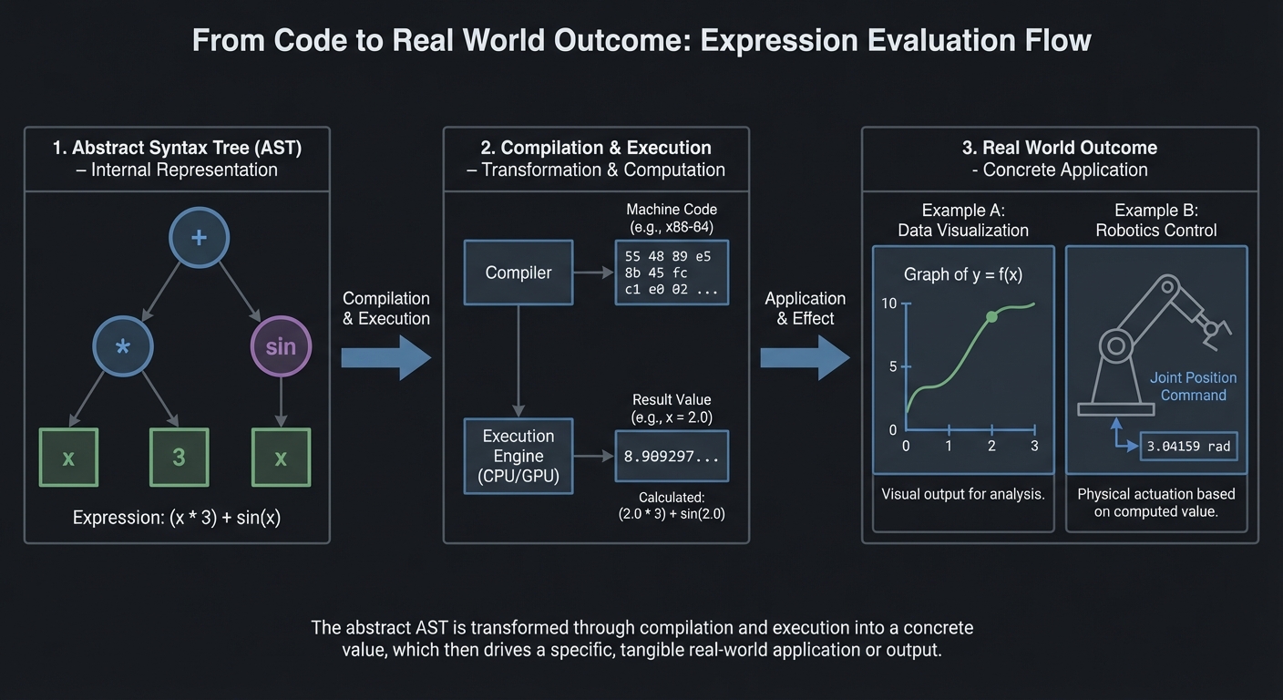
Derivative rules become recursive tree transformations:
deriv(x) = 1deriv(constant) = 0deriv(a + b) = deriv(a) + deriv(b)deriv(a * b) = deriv(a)*b + a*deriv(b)[product rule]deriv(f(g(x))) = deriv_f(g(x)) * deriv(g(x))[chain rule]
The chain rule is crucial for ML: backpropagation is just the chain rule applied repeatedly!
Learning milestones:
- Polynomial derivatives work → You’ve mastered the power rule
- Product and quotient rules work → You understand how derivatives distribute
- Chain rule handles nested functions → You understand composition (critical for backprop!)
The Core Question You Are Answering
How can a computer manipulate mathematical symbols rather than just numbers, and why is the chain rule the secret to computing derivatives of any composed function?
Numeric computation deals with specific values; symbolic computation deals with abstract expressions. When you implement symbolic differentiation, you are teaching a computer to apply the rules of calculus that you learned by hand. The chain rule is the master key: any complicated function is just simple functions nested inside each other, and the chain rule tells you how to peel back the layers. This is not just an exercise–automatic differentiation (used in every deep learning framework) is a descendant of these ideas.
Concepts You Must Understand First
Stop and research these before coding:
- Expression trees and recursive structure of mathematical expressions
- Why is
3 + 4 * 5naturally represented as a tree? - How does the tree structure encode operator precedence?
- Why is recursion the natural way to evaluate and transform expression trees?
- Book Reference: “SICP” Section 2.3.2 - Abelson & Sussman
- Why is
- The derivative rules and when to apply each
- Power rule: d/dx[x^n] = n*x^(n-1)
- Sum rule: d/dx[f+g] = df/dx + dg/dx
- Product rule: d/dx[f*g] = f’g + fg’
- Quotient rule: d/dx[f/g] = (f’g - fg’)/g^2
- Book Reference: “Calculus” Chapter 3 - James Stewart
- The chain rule: the key to composed functions
- If y = f(g(x)), then dy/dx = f’(g(x)) * g’(x)
- Why multiply the derivatives? Think about rates of change.
- How to apply the chain rule to triple composition f(g(h(x)))?
- Book Reference: “Calculus” Chapter 3.4 - James Stewart
- Derivatives of transcendental functions
- d/dx[sin(x)] = cos(x)
- d/dx[cos(x)] = -sin(x)
- d/dx[exp(x)] = exp(x)
- d/dx[ln(x)] = 1/x
- Book Reference: “Math for Programmers” Chapter 8 - Paul Orland
- Expression simplification: a hard problem
- Why does derivative output often look ugly (0x + 1y)?
- What simplification rules help? (0x = 0, 1x = x, x+0 = x)
- Why is full algebraic simplification actually very hard?
- Book Reference: “Computer Algebra” Chapter 1 - Geddes et al.
Questions to Guide Your Design
Before implementing, think through these:
-
How will you represent expressions? Classes for each operator type? Nested tuples? Strings with parsing? Each has trade-offs.
-
How will you distinguish x from constants? You need to know that d/dx[x] = 1 but d/dx[3] = 0. How is this represented?
-
How will you handle the chain rule? When you encounter sin(2x), you need to recognize it as sin(u) where u = 2x, compute d/du[sin(u)] = cos(u), then multiply by du/dx = 2.
-
What is your simplification strategy? Simplify during differentiation? After? Recursively? How much simplification is “enough”?
-
How will you output the result? As a new expression tree? As a string? In what notation?
-
How will you test correctness? Compare symbolic result to numerical derivative at random points?
Thinking Exercise
Before writing any code, manually trace the derivative of sin(x^2):
Expression tree:
    sin
     |
    pow
    / \
   x   2

Step 1: Recognize this is sin(u) where u = x^2
        Need chain rule: d/dx[sin(u)] = cos(u) * du/dx

Step 2: Compute d/du[sin(u)] = cos(u) = cos(x^2)

Step 3: Compute du/dx = d/dx[x^2]
        This is pow(x, 2), apply power rule: 2*x^1 = 2*x

Step 4: Apply chain rule: cos(x^2) * 2*x

Step 5: Simplify (optional): 2*x*cos(x^2)

Result tree:
        *
       / \
      2   *
         / \
        x  cos
            |
           pow
           / \
          x   2
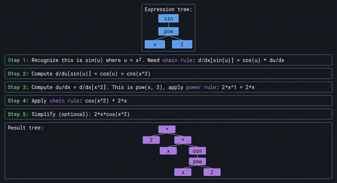
Now verify numerically: at x=1, derivative should be 21cos(1) = 1.08. Numerical approximation: (sin(1.001^2) - sin(0.999^2)) / 0.002 = 1.08. Correct!
The Interview Questions They Will Ask
-
“How would you implement a symbolic derivative calculator?” Expected answer: Represent expressions as trees, apply derivative rules recursively. The chain rule handles function composition.
-
“Walk me through differentiating
exp(x^2)symbolically.” Expected answer: This is exp(u) where u = x^2. Derivative of exp(u) is exp(u). Derivative of x^2 is 2x. By chain rule: exp(x^2) * 2x = 2x*exp(x^2). -
“What is the chain rule and why is it fundamental?” Expected answer: d/dx[f(g(x))] = f’(g(x)) * g’(x). It lets us differentiate any composed function by breaking it into inner and outer parts.
-
“How does symbolic differentiation differ from numerical differentiation?” Expected answer: Symbolic gives an exact formula; numerical gives an approximation at specific points. Symbolic is more general but harder to implement. Symbolic can be simplified; numerical cannot.
-
“What is the connection between symbolic differentiation and backpropagation?” Expected answer: Both apply the chain rule to compute derivatives of composed functions. Backprop is a form of automatic differentiation, which is related to but different from symbolic differentiation.
-
“How do you handle the product rule in an expression tree?” Expected answer: For ab, create a new tree: (deriv(a)b) + (a*deriv(b)). Recursively differentiate the subexpressions.
Hints in Layers
Hint 1: Use Python classes for your expression tree:
class Var:  # Represents x
    pass
class Const:  # Represents a number
    def __init__(self, value): self.value = value
class Add:
    def __init__(self, left, right): ...
class Mul:
    def __init__(self, left, right): ...
class Sin:
    def __init__(self, arg): ...
Hint 2: The derivative function is a big recursive pattern match:
def deriv(expr):
    if isinstance(expr, Var):
        return Const(1)
    elif isinstance(expr, Const):
        return Const(0)
    elif isinstance(expr, Add):
        return Add(deriv(expr.left), deriv(expr.right))
    elif isinstance(expr, Mul):
        # Product rule
        return Add(
            Mul(deriv(expr.left), expr.right),
            Mul(expr.left, deriv(expr.right))
        )
    # etc.
Hint 3: For chain rule (e.g., sin(f(x))):
elif isinstance(expr, Sin):
    # d/dx[sin(f)] = cos(f) * f'
    return Mul(Cos(expr.arg), deriv(expr.arg))
Hint 4: Basic simplification:
def simplify(expr):
    if isinstance(expr, Mul):
        left, right = simplify(expr.left), simplify(expr.right)
        if isinstance(left, Const) and left.value == 0:
            return Const(0)
        if isinstance(left, Const) and left.value == 1:
            return right
        # ... more rules
Hint 5: Test with numerical differentiation:
def numerical_deriv(f, x, eps=1e-7):
    return (f(x + eps) - f(x - eps)) / (2 * eps)

# Compare to your symbolic result evaluated at x
Books That Will Help
| Topic | Book | Chapter |
|---|---|---|
| Expression Trees | “SICP” - Abelson & Sussman | Section 2.3 |
| Derivative Rules | “Calculus” - James Stewart | Chapter 3 |
| Chain Rule Deep Dive | “Calculus” - James Stewart | Chapter 3.4 |
| Symbolic Computation | “Computer Algebra” - Geddes et al. | Chapter 1 |
| Pattern Matching | “Language Implementation Patterns” - Terence Parr | Chapter 4 |
| Automatic Differentiation | “Deep Learning” - Goodfellow et al. | Chapter 6 |
| Practical Applications | “Math for Programmers” - Paul Orland | Chapter 8 |
Common Pitfalls and Debugging
Problem 1: “Outputs drift after a few iterations”
- Why: Hidden numerical instability (unscaled features, aggressive step size, or repeated subtraction of nearly equal values).
- Fix: Normalize inputs, reduce step size, and track relative error rather than only absolute error.
- Quick test: Run the same task with two scales of input (for example x and 10x) and compare normalized error curves.
Problem 2: “Results are inconsistent across runs”
- Why: Random seeds, data split randomness, or non-deterministic ordering are uncontrolled.
- Fix: Set seeds, log configuration, and store split indices and hyperparameters with each run.
- Quick test: Re-run three times with the same seed and confirm metrics remain inside a tight tolerance band.
Problem 3: “The project works on the demo case but fails on edge cases”
- Why: Tests only cover happy-path inputs.
- Fix: Add adversarial inputs (empty values, extreme ranges, near-singular matrices, rare classes).
- Quick test: Build an edge-case test matrix and ensure every scenario reports expected behavior.
Definition of Done
- Core functionality works on reference inputs
- Edge cases are tested and documented
- Results are reproducible (seeded and versioned configuration)
- Performance or convergence behavior is measured and explained
- A short retrospective explains what failed first and how you fixed it
Project 9: Gradient Descent Visualizer
- File: P09-gradient-descent-visualizer.md
- Main Programming Language: Python
- Alternative Programming Languages: JavaScript, Julia, C++
- Coolness Level: Level 4: Hardcore Tech Flex
- Business Potential: 1. The “Resume Gold” (Educational/Personal Brand)
- Difficulty: Level 3: Advanced (The Engineer)
- Knowledge Area: Optimization / Multivariate Calculus
- Software or Tool: Optimization Visualizer
- Main Book: “Hands-On Machine Learning” by Aurélien Géron
What you’ll build: A visual tool that shows gradient descent finding the minimum of functions. Start with 1D functions, then 2D functions with contour plots showing the optimization path.
Why it teaches calculus: Gradient descent is the core algorithm of modern ML. Understanding it requires understanding derivatives (1D) and gradients (multi-D). Watching it converge (or diverge, or oscillate) builds intuition for learning rates and optimization landscapes.
Core challenges you’ll face:
- Computing numerical gradients → maps to partial derivatives
- Implementing gradient descent update → maps to θ = θ - α∇f(θ)
- Visualizing 2D functions as contour plots → maps to level curves
- Learning rate effects → maps to convergence behavior
- Local minima vs global minima → maps to non-convex optimization
Key Concepts:
- Gradients and Partial Derivatives: “Math for Programmers” Chapter 12 - Paul Orland
- Gradient Descent: “Hands-On Machine Learning” Chapter 4 - Aurélien Géron
- Optimization Landscapes: “Deep Learning” Chapter 4 - Goodfellow et al.
- Learning Rate Tuning: “Neural Networks and Deep Learning” Chapter 3 - Michael Nielsen
Difficulty: Advanced Time estimate: 2 weeks Prerequisites: Project 8, understanding of derivatives
Real World Outcome
$ python gradient_viz.py "x^2" --start=5 --lr=0.1

Optimizing f(x) = x²
Starting at x = 5.0
Learning rate α = 0.1

Step 0: x = 5.000, f(x) = 25.000, gradient = 10.000
Step 1: x = 4.000, f(x) = 16.000, gradient = 8.000
Step 2: x = 3.200, f(x) = 10.240, gradient = 6.400
...
Step 50: x = 0.001, f(x) = 0.000, gradient ≈ 0

[Animation: ball rolling down parabola, slowing as it approaches minimum]

$ python gradient_viz.py "sin(x)*x^2" --start=3

[Shows function with multiple local minima]
[Gradient descent gets stuck in local minimum!]
[Try different starting points to find global minimum]

$ python gradient_viz.py "x^2 + y^2" --start="(5,5)" --2d

[Contour plot with gradient descent path spiraling toward origin]
[Shows gradient vectors at each step pointing "downhill"]
Implementation Hints:
Numerical gradient: df/dx ≈ (f(x+ε) - f(x-ε)) / (2ε) where ε is small (e.g., 1e-7).
Gradient descent update: x_new = x_old - learning_rate * gradient
For 2D, compute partial derivatives separately:
∂f/∂x ≈ (f(x+ε, y) - f(x-ε, y)) / (2ε)
∂f/∂y ≈ (f(x, y+ε) - f(x, y-ε)) / (2ε)
gradient = [∂f/∂x, ∂f/∂y]
The gradient always points in the direction of steepest ascent, so we subtract to descend.
Learning milestones:
- 1D optimization converges → You understand gradient descent basics
- 2D contour plot shows path to minimum → You understand gradients geometrically
- You can explain why learning rate matters → You understand convergence dynamics
The Core Question You Are Answering
How can an algorithm find the bottom of a valley by only knowing the local slope, and why does this simple idea power all of modern machine learning?
Gradient descent embodies a beautiful idea: to minimize a function, take small steps opposite to the gradient (the direction of steepest ascent). You do not need to know the global shape of the landscape–just the local slope tells you which way is “down.” This local-to-global strategy is the engine behind training neural networks, fitting statistical models, and solving optimization problems with millions of parameters. Understanding gradient descent deeply means understanding how machines learn.
Concepts You Must Understand First
Stop and research these before coding:
- What is a gradient and how does it generalize the derivative?
- For f(x,y), the gradient is [df/dx, df/dy]. What does this vector represent geometrically?
- Why does the gradient point in the direction of steepest ascent?
- What is the relationship between gradient and directional derivative?
- Book Reference: “Calculus: Early Transcendentals” Chapter 14 - James Stewart
- The numerical gradient: finite difference approximation
- Why does (f(x+h) - f(x-h))/(2h) approximate f’(x)?
- Why is central difference better than forward difference?
- What happens when h is too small (numerical precision) or too large (inaccuracy)?
- Book Reference: “Numerical Recipes” Chapter 5 - Press et al.
- The gradient descent update rule and its geometric meaning
- theta_new = theta_old - alpha * gradient
- Why subtract (not add) the gradient?
- What is the learning rate alpha and why does it matter?
- Book Reference: “Hands-On Machine Learning” Chapter 4 - Aurelien Geron
- Convergence: when does gradient descent work well?
- What is a convex function and why is it easy to optimize?
- What are local minima and saddle points?
- What conditions guarantee convergence?
- Book Reference: “Deep Learning” Chapter 4 - Goodfellow et al.
- The learning rate dilemma
- Too large: overshooting, divergence, oscillation
- Too small: slow convergence, getting stuck
- Adaptive learning rates: why do methods like Adam help?
- Book Reference: “Neural Networks and Deep Learning” Chapter 3 - Michael Nielsen
- Contour plots and level curves
- What does a contour plot show about a 2D function?
- How can you read the gradient direction from contours?
- What do elliptical vs circular contours tell you about the function?
- Book Reference: “Math for Programmers” Chapter 12 - Paul Orland
Questions to Guide Your Design
Before implementing, think through these:
-
How will you compute numerical gradients? Central difference is more accurate but requires 2n function evaluations for n dimensions. Is this acceptable?
-
How will you handle different dimensionalities? 1D is a curve, 2D can be shown as contours, 3D and beyond cannot be visualized directly. What do you show?
-
What stopping conditions will you use? When gradient is near zero? When change in x is small? After maximum iterations? All of these?
-
How will you visualize the optimization path? Animate the point moving? Draw trajectory? Show gradient vectors?
-
What interesting functions will you include? Paraboloids, Rosenbrock’s banana function, Himmelblau’s function with multiple minima?
-
How will you demonstrate learning rate effects? Side-by-side comparisons? Interactive slider?
Thinking Exercise
Before writing any code, trace gradient descent by hand:
Minimize f(x) = x^2 starting at x = 5 with learning rate 0.1:
Derivative: f'(x) = 2x

Step 0: x = 5.000
        gradient = 2 * 5 = 10
        x_new = 5 - 0.1 * 10 = 4.000
        f(x_new) = 16.000

Step 1: x = 4.000
        gradient = 2 * 4 = 8
        x_new = 4 - 0.1 * 8 = 3.200
        f(x_new) = 10.240

Step 2: x = 3.200
        gradient = 2 * 3.2 = 6.4
        x_new = 3.2 - 0.1 * 6.4 = 2.560
        f(x_new) = 6.554

...continuing...

Step 10: x = 0.537, f(x) = 0.288
Step 20: x = 0.058, f(x) = 0.003
Step 30: x = 0.006, f(x) = 0.00004
Notice: x decreases by a factor of (1 - 0.2) = 0.8 each step. This is because for f(x) = x^2, gradient descent with learning rate alpha gives x_new = x(1 - 2*alpha).
The Interview Questions They Will Ask
-
“What is gradient descent and why is it used in machine learning?” Expected answer: An iterative optimization algorithm that moves toward a minimum by taking steps proportional to the negative gradient. Used because most ML problems involve minimizing loss functions.
-
“Why do we subtract the gradient instead of adding it?” Expected answer: The gradient points toward the steepest ascent. We want to descend, so we go in the opposite direction.
-
“What happens if the learning rate is too large? Too small?” Expected answer: Too large causes overshooting and possibly divergence (oscillating or exploding). Too small causes very slow convergence and can get stuck.
-
“What is the difference between gradient descent and stochastic gradient descent?” Expected answer: GD uses the full dataset to compute the gradient each step. SGD uses a random subset (mini-batch), which is noisier but much faster for large datasets.
-
“How does gradient descent handle local minima?” Expected answer: It can get stuck in local minima. Solutions include: random restarts, momentum, stochastic noise, or using convex problems where all local minima are global.
-
“What is the role of convexity in optimization?” Expected answer: Convex functions have a single global minimum. Gradient descent is guaranteed to find it. Non-convex functions have multiple local minima and saddle points, making optimization harder.
-
“How would you compute the gradient numerically?” Expected answer: Central difference: (f(x+h) - f(x-h))/(2h). For multivariate functions, compute each partial derivative separately.
Hints in Layers
Hint 1: Start with 1D optimization. Plot the function and animate a dot rolling down:
def gradient_descent_1d(f, x0, lr=0.1, n_steps=50):
    x = x0
    history = [x]
    for _ in range(n_steps):
        grad = (f(x + 1e-7) - f(x - 1e-7)) / (2e-7)
        x = x - lr * grad
        history.append(x)
    return history
Hint 2: For 2D visualization, use matplotlib contour plots:
import matplotlib.pyplot as plt
import numpy as np

x = np.linspace(-3, 3, 100)
y = np.linspace(-3, 3, 100)
X, Y = np.meshgrid(x, y)
Z = X**2 + Y**2  # Paraboloid

plt.contour(X, Y, Z, levels=20)
plt.plot(path_x, path_y, 'r.-')  # Overlay path
Hint 3: For 2D numerical gradient:
def gradient_2d(f, x, y, h=1e-7):
    df_dx = (f(x + h, y) - f(x - h, y)) / (2 * h)
    df_dy = (f(x, y + h) - f(x, y - h)) / (2 * h)
    return np.array([df_dx, df_dy])
Hint 4: Interesting test functions:
- Paraboloid: f(x,y) = x^2 + y^2 (easy, single minimum at origin)
- Elliptical: f(x,y) = x^2 + 10*y^2 (harder, elongated contours)
- Rosenbrock: f(x,y) = (1-x)^2 + 100*(y-x^2)^2 (very hard, curved valley)
Hint 5: To show learning rate effects, run the same optimization with different learning rates and overlay the paths on the same contour plot. Color-code by learning rate.
Books That Will Help
| Topic | Book | Chapter |
|---|---|---|
| Gradient Fundamentals | “Calculus: Early Transcendentals” - James Stewart | Chapter 14 |
| Gradient Descent Algorithm | “Hands-On Machine Learning” - Aurelien Geron | Chapter 4 |
| Optimization Theory | “Deep Learning” - Goodfellow et al. | Chapter 4 |
| Learning Rate and Convergence | “Neural Networks and Deep Learning” - Michael Nielsen | Chapter 3 |
| Numerical Methods | “Numerical Recipes” - Press et al. | Chapter 10 |
| Convex Optimization | “Convex Optimization” - Boyd & Vandenberghe | Chapter 9 |
| Visualization | “Math for Programmers” - Paul Orland | Chapter 12 |
Common Pitfalls and Debugging
Problem 1: “Outputs drift after a few iterations”
- Why: Hidden numerical instability (unscaled features, aggressive step size, or repeated subtraction of nearly equal values).
- Fix: Normalize inputs, reduce step size, and track relative error rather than only absolute error.
- Quick test: Run the same task with two scales of input (for example x and 10x) and compare normalized error curves.
Problem 2: “Results are inconsistent across runs”
- Why: Random seeds, data split randomness, or non-deterministic ordering are uncontrolled.
- Fix: Set seeds, log configuration, and store split indices and hyperparameters with each run.
- Quick test: Re-run three times with the same seed and confirm metrics remain inside a tight tolerance band.
Problem 3: “The project works on the demo case but fails on edge cases”
- Why: Tests only cover happy-path inputs.
- Fix: Add adversarial inputs (empty values, extreme ranges, near-singular matrices, rare classes).
- Quick test: Build an edge-case test matrix and ensure every scenario reports expected behavior.
Definition of Done
- Core functionality works on reference inputs
- Edge cases are tested and documented
- Results are reproducible (seeded and versioned configuration)
- Performance or convergence behavior is measured and explained
- A short retrospective explains what failed first and how you fixed it
Project 10: Numerical Integration Visualizer
- File: P10-numerical-integration-visualizer.md
- Main Programming Language: Python
- Alternative Programming Languages: C, Julia, Rust
- Coolness Level: Level 3: Genuinely Clever
- Business Potential: 1. The “Resume Gold” (Educational/Personal Brand)
- Difficulty: Level 2: Intermediate (The Developer)
- Knowledge Area: Numerical Methods / Calculus
- Software or Tool: Integration Calculator
- Main Book: “Numerical Recipes” by Press et al.
What you’ll build: A tool that computes definite integrals numerically using various methods (rectangles, trapezoids, Simpson’s rule), visualizing the approximation and error.
Why it teaches calculus: Integration is about accumulating infinitely many infinitesimal pieces. Implementing numerical integration shows you what the integral means geometrically (area under curve) and how approximations converge to the true value.
Core challenges you’ll face:
- Riemann sums (rectangles) → maps to basic integration concept
- Trapezoidal rule → maps to linear interpolation
- Simpson’s rule → maps to quadratic interpolation
- Error analysis → maps to how approximations converge
- Adaptive integration → maps to concentrating effort where needed
Key Concepts:
- Definite Integrals: “Calculus” Chapter 5 - James Stewart
- Numerical Integration: “Numerical Recipes” Chapter 4 - Press et al.
- Error Analysis: “Algorithms” Section 5.8 - Sedgewick & Wayne
- Riemann Sums: “Math for Programmers” Chapter 8 - Paul Orland
Difficulty: Intermediate Time estimate: 1 week Prerequisites: Understanding of what integration means
Real World Outcome
$ python integrate.py "x^2" 0 3

Computing ∫₀³ x² dx

Method        | n=10    | n=100   | n=1000  | Exact
--------------+---------+---------+---------+-------
Left Riemann  | 7.785   | 8.866   | 8.987   | 9.000
Right Riemann | 10.395  | 9.136   | 9.014   | 9.000
Trapezoidal   | 9.090   | 9.001   | 9.000   | 9.000
Simpson's     | 9.000   | 9.000   | 9.000   | 9.000

[Visual: Area under x² from 0 to 3, with rectangles/trapezoids overlaid]
[Animation: More rectangles → better approximation]
Implementation Hints: Left Riemann sum:
def left_riemann(f, a, b, n):
    dx = (b - a) / n
    return sum(f(a + i*dx) * dx for i in range(n))
Trapezoidal: (f(left) + f(right)) / 2 * dx for each interval
Simpson’s rule (for even n):
∫f ≈ (dx/3) * [f(x₀) + 4f(x₁) + 2f(x₂) + 4f(x₃) + ... + f(xₙ)]
(alternating 4s and 2s, 1s at ends)
Learning milestones:
- Rectangles approximate area → You understand integration geometrically
- More rectangles = better approximation → You understand limits
- Simpson’s converges much faster → You understand higher-order methods
The Core Question You Are Answering
How can we compute the area under any curve when we cannot find an antiderivative, and why do different approximation methods converge at dramatically different rates?
Integration is fundamentally about accumulation–adding up infinitely many infinitesimally small pieces. When exact antiderivatives are unavailable (which is most of the time for real-world functions), we approximate by summing finite rectangles, trapezoids, or parabolas. The profound insight is that different approximation strategies converge to the true value at vastly different speeds. Simpson’s rule uses parabolas and achieves O(h^4) accuracy, while rectangles give only O(h). Understanding this prepares you for the numerical methods that underpin scientific computing.
Concepts You Must Understand First
Stop and research these before coding:
- The definite integral as a limit of Riemann sums
- What does the integral symbol mean geometrically?
- Why is the limit of the sum as rectangles get infinitely thin equal to the area?
- What are left, right, and midpoint Riemann sums?
- Book Reference: “Calculus” Chapter 5 - James Stewart
- The trapezoidal rule: using linear interpolation
- Why is a trapezoid a better approximation than a rectangle?
- What is the formula for the trapezoidal rule?
- What is the error order (O(h^2))?
- Book Reference: “Numerical Recipes” Chapter 4 - Press et al.
- Simpson’s rule: using quadratic interpolation
- Why does fitting a parabola through three points give better accuracy?
- What is the 1-4-1 weighting pattern?
- Why does Simpson’s rule require an even number of intervals?
- Book Reference: “Numerical Recipes” Chapter 4 - Press et al.
- Error analysis: why higher-order methods are better
- What does O(h^n) error mean for convergence?
- Why does Simpson’s rule (O(h^4)) need far fewer points than rectangles (O(h))?
- When might higher-order methods NOT be better?
- Book Reference: “Numerical Methods” Chapter 7 - Burden & Faires
- Adaptive integration: concentrating effort where needed
- Why use more subintervals where the function changes rapidly?
- What is the basic idea of adaptive quadrature?
- How do you estimate local error to guide adaptation?
- Book Reference: “Numerical Recipes” Chapter 4 - Press et al.
Questions to Guide Your Design
Before implementing, think through these:
-
How will you represent the function to integrate? Lambda functions? Strings that get parsed? Callable objects?
-
How will you handle functions with singularities or discontinuities? Division by zero at endpoints? Jump discontinuities?
-
What comparison metrics will you show? Error vs. n? Computation time? Visual accuracy?
-
How will you visualize each method? Overlaid rectangles/trapezoids on the function? Separate plots?
-
Will you implement adaptive integration? This is more complex but shows the power of error estimation.
-
How will you handle the “exact” value for comparison? Use scipy.integrate.quad as ground truth? Symbolic integration when possible?
Thinking Exercise
Before writing any code, compute the integral of x^2 from 0 to 3 by hand using each method with n=2:
True value: integral of x^2 from 0 to 3 = [x^3/3] from 0 to 3 = 27/3 = 9.0
Left Riemann (n=2):
  Interval width: h = (3-0)/2 = 1.5
  Left endpoints: x = 0, x = 1.5
  f(0) = 0, f(1.5) = 2.25
  Sum = (0 + 2.25) * 1.5 = 3.375
  Error = |9 - 3.375| = 5.625

Right Riemann (n=2):
  Right endpoints: x = 1.5, x = 3
  f(1.5) = 2.25, f(3) = 9
  Sum = (2.25 + 9) * 1.5 = 16.875
  Error = |9 - 16.875| = 7.875

Trapezoidal (n=2):
  Average of left and right = (3.375 + 16.875) / 2 = 10.125
  Or: h/2 * [f(0) + 2*f(1.5) + f(3)] = 1.5/2 * [0 + 4.5 + 9] = 10.125
  Error = |9 - 10.125| = 1.125  (Much better!)

Simpson's (n=2):
  Uses parabola through (0,0), (1.5, 2.25), (3, 9)
  = h/3 * [f(0) + 4*f(1.5) + f(3)] = 1.5/3 * [0 + 9 + 9] = 9.0
  Error = 0  (Exact! Simpson's is exact for polynomials up to degree 3)
This example shows why Simpson’s rule is so powerful!
The Interview Questions They Will Ask
-
“What is numerical integration and when do you need it?” Expected answer: Approximating the definite integral when no closed-form antiderivative exists, or when the function is only known at discrete points.
-
“Explain the difference between left Riemann sums, trapezoidal rule, and Simpson’s rule.” Expected answer: Left Riemann uses rectangles with height at left endpoint (O(h) error). Trapezoidal uses trapezoids (linear interpolation, O(h^2) error). Simpson’s uses parabolas (quadratic interpolation, O(h^4) error).
-
“Why does Simpson’s rule converge faster than the trapezoidal rule?” Expected answer: Simpson’s uses higher-order polynomial approximation (quadratics vs. lines). The error terms cancel out more effectively, giving O(h^4) vs O(h^2).
-
“What is adaptive integration?” Expected answer: Using more subintervals where the function changes rapidly and fewer where it is smooth. Based on local error estimation.
-
“When might the trapezoidal rule outperform Simpson’s rule?” Expected answer: When the function has discontinuities or sharp corners that violate smoothness assumptions. Also when function evaluations are very expensive and the higher accuracy does not justify extra points.
-
“How do you verify the correctness of a numerical integration routine?” Expected answer: Test on functions with known integrals. Check that doubling n reduces error by the expected factor (h becomes h/2, so O(h^4) error should drop by 16x for Simpson’s).
Hints in Layers
Hint 1: Start with the three basic implementations:
def left_riemann(f, a, b, n):
    h = (b - a) / n
    return h * sum(f(a + i*h) for i in range(n))

def trapezoidal(f, a, b, n):
    h = (b - a) / n
    return h * (0.5*f(a) + sum(f(a + i*h) for i in range(1, n)) + 0.5*f(b))

def simpsons(f, a, b, n):  # n must be even
    h = (b - a) / n
    x = [a + i*h for i in range(n+1)]
    return h/3 * (f(a) + f(b) +
                  4*sum(f(x[i]) for i in range(1, n, 2)) +
                  2*sum(f(x[i]) for i in range(2, n-1, 2)))
Hint 2: For visualization, draw rectangles/trapezoids:
import matplotlib.pyplot as plt
import matplotlib.patches as patches

# For rectangles
for i in range(n):
    x_left = a + i*h
    rect = patches.Rectangle((x_left, 0), h, f(x_left), ...)
    ax.add_patch(rect)
Hint 3: Create a convergence plot:
ns = [2, 4, 8, 16, 32, 64, 128, 256]
errors = [abs(simpsons(f, a, b, n) - true_value) for n in ns]
plt.loglog(ns, errors, 'o-')  # Log-log shows power law clearly
Hint 4: Good test functions:
- x^2 from 0 to 1 (exact = 1/3, smooth)
- sin(x) from 0 to pi (exact = 2, smooth periodic)
- sqrt(x) from 0 to 1 (exact = 2/3, infinite derivative at 0)
- 1/(1+x^2) from 0 to 1 (exact = pi/4, smooth but interesting)
Hint 5: For adaptive integration, the basic idea:
def adaptive(f, a, b, tol):
    mid = (a + b) / 2
    whole = simpsons(f, a, b, 2)
    left = simpsons(f, a, mid, 2)
    right = simpsons(f, mid, b, 2)
    if abs(whole - (left + right)) < tol:
        return left + right
    else:
        return adaptive(f, a, mid, tol/2) + adaptive(f, mid, b, tol/2)
Books That Will Help
| Topic | Book | Chapter |
|---|---|---|
| Riemann Sums and Theory | “Calculus” - James Stewart | Chapter 5 |
| Numerical Integration Methods | “Numerical Recipes” - Press et al. | Chapter 4 |
| Error Analysis | “Numerical Methods” - Burden & Faires | Chapter 4 |
| Adaptive Quadrature | “Numerical Recipes” - Press et al. | Chapter 4 |
| Gaussian Quadrature | “Numerical Linear Algebra” - Trefethen & Bau | Chapter 19 |
| Applications in ML | “Pattern Recognition and ML” - Bishop | Appendix A |
| Visualization | “Math for Programmers” - Paul Orland | Chapter 8 |
Common Pitfalls and Debugging
Problem 1: “Outputs drift after a few iterations”
- Why: Hidden numerical instability (unscaled features, aggressive step size, or repeated subtraction of nearly equal values).
- Fix: Normalize inputs, reduce step size, and track relative error rather than only absolute error.
- Quick test: Run the same task with two scales of input (for example x and 10x) and compare normalized error curves.
Problem 2: “Results are inconsistent across runs”
- Why: Random seeds, data split randomness, or non-deterministic ordering are uncontrolled.
- Fix: Set seeds, log configuration, and store split indices and hyperparameters with each run.
- Quick test: Re-run three times with the same seed and confirm metrics remain inside a tight tolerance band.
Problem 3: “The project works on the demo case but fails on edge cases”
- Why: Tests only cover happy-path inputs.
- Fix: Add adversarial inputs (empty values, extreme ranges, near-singular matrices, rare classes).
- Quick test: Build an edge-case test matrix and ensure every scenario reports expected behavior.
Definition of Done
- Core functionality works on reference inputs
- Edge cases are tested and documented
- Results are reproducible (seeded and versioned configuration)
- Performance or convergence behavior is measured and explained
- A short retrospective explains what failed first and how you fixed it
Project 11: Backpropagation from Scratch (Single Neuron)
- File: P11-backpropagation-from-scratch-single-neuron.md
- Main Programming Language: Python
- Alternative Programming Languages: C, Julia, Rust
- Coolness Level: Level 4: Hardcore Tech Flex
- Business Potential: 1. The “Resume Gold” (Educational/Personal Brand)
- Difficulty: Level 3: Advanced (The Engineer)
- Knowledge Area: Neural Networks / Calculus
- Software or Tool: Backprop Engine
- Main Book: “Neural Networks and Deep Learning” by Michael Nielsen
What you’ll build: A single neuron that learns via backpropagation. This is the atomic unit of neural networks. You’ll implement forward pass, loss calculation, and backward pass (gradient computation via chain rule) completely from scratch.
Why it teaches calculus: Backpropagation IS the chain rule. Understanding how gradients flow backward through a computation graph is the key insight of deep learning. Building this from scratch demystifies what frameworks like PyTorch do automatically.
Core challenges you’ll face:
- Forward pass computation → maps to function composition
- Loss function (MSE or cross-entropy) → maps to measuring error
- Computing ∂L/∂w via chain rule → maps to backpropagation
- Weight update via gradient descent → maps to optimization
- Sigmoid/ReLU derivatives → maps to activation function gradients
Key Concepts:
- Chain Rule: “Calculus” Chapter 3 - James Stewart
- Backpropagation Algorithm: “Neural Networks and Deep Learning” Chapter 2 - Michael Nielsen
- Computational Graphs: “Deep Learning” Chapter 6 - Goodfellow et al.
- Gradient Flow: “Hands-On Machine Learning” Chapter 10 - Aurélien Géron
Difficulty: Advanced Time estimate: 1-2 weeks Prerequisites: Project 8, Project 9, understanding of chain rule
Real World Outcome
$ python neuron.py

Training single neuron to learn AND gate:
Inputs: [[0,0], [0,1], [1,0], [1,1]]
Targets: [0, 0, 0, 1]

Initial weights: w1=0.5, w2=-0.3, bias=-0.1
Initial predictions: [0.475, 0.377, 0.549, 0.450]
Initial loss: 0.312

Epoch 100:
  Forward:  input=[1,1] → z = 1*0.8 + 1*0.7 + (-0.5) = 1.0 → σ(1.0) = 0.731
  Loss:     (0.731 - 1)² = 0.072
  Backward: ∂L/∂z = 2(0.731-1) * σ'(1.0) = -0.106
            ∂L/∂w1 = -0.106 * 1 = -0.106  [input was 1]
            ∂L/∂w2 = -0.106 * 1 = -0.106
  Update:   w1 += 0.1 * 0.106 = 0.811

Epoch 1000:
  Predictions: [0.02, 0.08, 0.07, 0.91]  ✓ (AND gate learned!)
  Final weights: w1=5.2, w2=5.1, bias=-7.8

[Visual: Decision boundary moving during training]
Implementation Hints: Neuron computation:
z = w1*x1 + w2*x2 + bias  (linear combination)
a = sigmoid(z) = 1 / (1 + exp(-z))  (activation)
Sigmoid derivative: sigmoid'(z) = sigmoid(z) * (1 - sigmoid(z))
Chain rule for weight gradient:
∂L/∂w1 = ∂L/∂a * ∂a/∂z * ∂z/∂w1
       = 2(a - target) * sigmoid'(z) * x1
This is backpropagation! The gradient “flows backward” through the computation.
Learning milestones:
- Forward pass produces output → You understand function composition
- Gradients computed correctly → You’ve mastered the chain rule
- Neuron learns the AND gate → You’ve implemented learning from scratch!
The Core Question You Are Answering
How does a machine “learn” from its mistakes?
When you train a neuron, you’re answering one of the most profound questions in machine learning: how can an algorithm improve itself by measuring how wrong it was? The answer lies in the beautiful connection between calculus (the chain rule) and optimization (gradient descent). Every time your neuron updates its weights, it’s answering: “In which direction should I change to be less wrong next time?”
Concepts You Must Understand First
Stop and research these before coding:
- The Forward Pass as Function Composition
- What does it mean to “compose” two functions like f(g(x))?
- Why is a neuron just a composition of a linear function and an activation?
- How do you trace an input through multiple operations to get an output?
- Book Reference: “Neural Networks and Deep Learning” Chapter 1 - Michael Nielsen
- Loss Functions and Their Purpose
- Why do we need a single number to represent “how wrong” we are?
- What’s the difference between MSE and cross-entropy loss? When use each?
- Why does squaring errors in MSE penalize large errors more than small ones?
- Book Reference: “Deep Learning” Chapter 3.13 - Goodfellow et al.
- The Chain Rule from Calculus
- If y = f(g(x)), how do you compute dy/dx?
- Why is the chain rule called “chain”? What’s being chained?
- Can you apply the chain rule to three or more nested functions?
- Book Reference: “Calculus” Chapter 3.4 - James Stewart
- Activation Functions and Their Derivatives
- Why does sigmoid(x) output values between 0 and 1?
- What is the derivative of sigmoid? Why is it sigmoid(x) * (1 - sigmoid(x))?
- What is ReLU and why is its derivative so simple?
- Where does the gradient “vanish” for sigmoid? Why is this a problem?
- Book Reference: “Neural Networks and Deep Learning” Chapter 3 - Michael Nielsen
- Gradient Descent Weight Updates
- Why do we subtract the gradient rather than add it?
- What role does the learning rate play? What happens if it’s too big/small?
- Why do we multiply the gradient by the input to get the weight gradient?
- Book Reference: “Hands-On Machine Learning” Chapter 4 - Aurelien Geron
Questions to Guide Your Design
Before implementing, think through these:
-
Data Representation: How will you represent inputs, weights, and the bias? As separate variables or bundled together?
-
Forward Pass Structure: What’s the exact sequence of operations? Linear combination first, then activation? How will you store intermediate values for the backward pass?
-
Loss Computation: Will you compute loss for each sample individually or as a batch? How does this affect your gradient calculation?
-
Backward Pass Flow: In what order do you compute derivatives? Start from the loss and work backward, or start from the inputs?
-
Weight Update Timing: Do you update weights after each sample, or accumulate gradients over a batch first?
-
Convergence Detection: How will you know when to stop training? Fixed epochs? When loss plateaus?
Thinking Exercise
Hand-trace this backpropagation before coding:
Given a single neuron with:
- Input: x = [1.0, 0.5]
- Weights: w = [0.3, -0.2]
- Bias: b = 0.1
- Target: y = 1
- Activation: sigmoid
Step 1: Forward Pass
z = w[0]*x[0] + w[1]*x[1] + b = ?
a = sigmoid(z) = 1 / (1 + exp(-z)) = ?
Step 2: Loss (MSE)
L = (a - y)^2 = ?
Step 3: Backward Pass
dL/da = 2 * (a - y) = ?
da/dz = sigmoid(z) * (1 - sigmoid(z)) = ?
dL/dz = dL/da * da/dz = ?

dz/dw[0] = x[0] = ?
dz/dw[1] = x[1] = ?
dz/db = 1

dL/dw[0] = dL/dz * dz/dw[0] = ?
dL/dw[1] = dL/dz * dz/dw[1] = ?
dL/db = dL/dz * 1 = ?
Step 4: Update (learning rate = 0.1)
w[0]_new = w[0] - 0.1 * dL/dw[0] = ?
w[1]_new = w[1] - 0.1 * dL/dw[1] = ?
b_new = b - 0.1 * dL/db = ?
Work through this completely by hand. Check: After update, does the neuron predict closer to 1?
The Interview Questions They Will Ask
- “What is backpropagation, and why is it efficient?”
- Expected: It’s applying the chain rule to compute gradients efficiently by reusing intermediate derivatives.
- “Walk me through the gradient computation for a single neuron with sigmoid activation.”
- Expected: Forward pass (z = wx + b, a = sigmoid(z)), loss, then chain rule backward.
- “Why do we use log loss (cross-entropy) instead of MSE for classification?”
- Expected: MSE gradients become very small when predictions are confident but wrong; cross-entropy doesn’t have this problem.
- “What is the vanishing gradient problem?”
- Expected: Sigmoid squashes outputs to (0,1), and its derivative is at most 0.25. Multiplying small numbers across many layers makes gradients vanishingly small.
- “Implement the backward pass for a neuron with ReLU activation.”
- Expected: dL/dz = dL/da * 1 if z > 0 else 0. Much simpler than sigmoid!
- “What happens if you initialize all weights to zero?”
- Expected: All neurons compute the same thing. Gradients are identical. They stay identical forever. Symmetry breaking is essential.
- “How does batch size affect gradient updates?”
- Expected: Larger batches give smoother, more accurate gradients but slower updates. Smaller batches are noisier but can escape local minima.
Hints in Layers
Hint 1: The Core Structure Your neuron has three learnable parameters: w1, w2 (weights for two inputs), and b (bias). The forward pass computes: z = w1x1 + w2x2 + b, then a = sigmoid(z). Start by getting this working.
Hint 2: The Loss and Its Derivative For MSE: L = (a - target)^2. The derivative dL/da = 2*(a - target). This is where the “error signal” starts.
Hint 3: The Chain Rule Application You need dL/dw1. By the chain rule: dL/dw1 = dL/da * da/dz * dz/dw1. You already have dL/da. Compute da/dz = a*(1-a) (sigmoid derivative). And dz/dw1 = x1 (the input!).
Hint 4: The Complete Gradient Flow
# Forward
z = w1*x1 + w2*x2 + b
a = 1 / (1 + np.exp(-z))

# Backward
dL_da = 2 * (a - target)
da_dz = a * (1 - a)
dL_dz = dL_da * da_dz  # This is the key "delta" term

dL_dw1 = dL_dz * x1
dL_dw2 = dL_dz * x2
dL_db = dL_dz * 1
Hint 5: The Training Loop
for epoch in range(1000):
    total_loss = 0
    for (x1, x2), target in training_data:
        # Forward pass
        # Compute loss
        # Backward pass
        # Update weights
        w1 -= learning_rate * dL_dw1
        w2 -= learning_rate * dL_dw2
        b -= learning_rate * dL_db
Books That Will Help
| Topic | Book | Chapter |
|---|---|---|
| Backpropagation Intuition | “Neural Networks and Deep Learning” | Chapter 2 - Michael Nielsen |
| Chain Rule Fundamentals | “Calculus” | Chapter 3 - James Stewart |
| Computational Graphs | “Deep Learning” | Chapter 6.5 - Goodfellow et al. |
| Loss Functions | “Deep Learning” | Chapter 3 - Goodfellow et al. |
| Sigmoid and Activation Functions | “Hands-On Machine Learning” | Chapter 10 - Aurelien Geron |
| Gradient Descent Variations | “Deep Learning” | Chapter 8 - Goodfellow et al. |
| Weight Initialization | “Neural Networks and Deep Learning” | Chapter 3 - Michael Nielsen |
Part 4: Probability & Statistics
ML is fundamentally about making predictions under uncertainty. Probability gives us the language to express and reason about uncertainty.
Common Pitfalls and Debugging
Problem 1: “Outputs drift after a few iterations”
- Why: Hidden numerical instability (unscaled features, aggressive step size, or repeated subtraction of nearly equal values).
- Fix: Normalize inputs, reduce step size, and track relative error rather than only absolute error.
- Quick test: Run the same task with two scales of input (for example x and 10x) and compare normalized error curves.
Problem 2: “Results are inconsistent across runs”
- Why: Random seeds, data split randomness, or non-deterministic ordering are uncontrolled.
- Fix: Set seeds, log configuration, and store split indices and hyperparameters with each run.
- Quick test: Re-run three times with the same seed and confirm metrics remain inside a tight tolerance band.
Problem 3: “The project works on the demo case but fails on edge cases”
- Why: Tests only cover happy-path inputs.
- Fix: Add adversarial inputs (empty values, extreme ranges, near-singular matrices, rare classes).
- Quick test: Build an edge-case test matrix and ensure every scenario reports expected behavior.
Definition of Done
- Core functionality works on reference inputs
- Edge cases are tested and documented
- Results are reproducible (seeded and versioned configuration)
- Performance or convergence behavior is measured and explained
- A short retrospective explains what failed first and how you fixed it
Project 12: Monte Carlo Pi Estimator
- File: P12-monte-carlo-pi-estimator.md
- Main Programming Language: Python
- Alternative Programming Languages: C, JavaScript, Rust
- Coolness Level: Level 3: Genuinely Clever
- Business Potential: 1. The “Resume Gold” (Educational/Personal Brand)
- Difficulty: Level 1: Beginner (The Tinkerer)
- Knowledge Area: Probability / Monte Carlo Methods
- Software or Tool: Pi Estimator
- Main Book: “Grokking Algorithms” by Aditya Bhargava
What you’ll build: A visual tool that estimates π by randomly throwing “darts” at a square containing a circle. The ratio of darts inside the circle to total darts approaches π/4.
Why it teaches probability: This introduces the fundamental Monte Carlo idea: using random sampling to estimate quantities. The law of large numbers in action—more samples = better estimate. This technique underpins Bayesian ML, reinforcement learning, and more.
Core challenges you’ll face:
- Generating uniform random points → maps to uniform distribution
- Checking if point is in circle → maps to geometric probability
- Convergence as sample size increases → maps to law of large numbers
- Estimating error bounds → maps to confidence intervals
- Visualizing the process → maps to sampling intuition
Key Concepts:
- Monte Carlo Methods: “Grokking Algorithms” Chapter 10 - Aditya Bhargava
- Law of Large Numbers: “All of Statistics” Chapter 5 - Larry Wasserman
- Uniform Distribution: “Math for Programmers” Chapter 15 - Paul Orland
- Geometric Probability: “Probability” Chapter 2 - Pitman
Difficulty: Beginner Time estimate: Weekend Prerequisites: Basic programming, understanding of randomness
Real World Outcome
$ python monte_carlo_pi.py 1000000

Throwing 1,000,000 random darts at a 2x2 square with inscribed circle...

Samples   | Inside Circle | Estimate of π | Error
----------+---------------+---------------+-------
100       | 79            | 3.160         | 0.6%
1,000     | 783           | 3.132         | 0.3%
10,000    | 7,859         | 3.144         | 0.08%
100,000   | 78,551        | 3.142         | 0.01%
1,000,000 | 785,426       | 3.1417        | 0.004%

Actual π = 3.14159265...

[Visual: Square with circle, dots accumulating, π estimate updating in real-time]
Implementation Hints:
import random

inside = 0
for _ in range(n):
    x = random.uniform(-1, 1)
    y = random.uniform(-1, 1)
    if x**2 + y**2 <= 1:  # Inside unit circle
        inside += 1

pi_estimate = 4 * inside / n
Why does this work? Area of circle = π·r² = π (for r=1). Area of square = 4. Ratio = π/4.
Error decreases as 1/√n (standard Monte Carlo convergence).
Learning milestones:
- Basic estimate works → You understand random sampling
- Estimate improves with more samples → You understand law of large numbers
- You can predict how many samples for desired accuracy → You understand convergence rates
The Core Question You Are Answering
Can randomness give us certainty?
This seems paradoxical: we’re using random numbers to compute something that’s completely deterministic (pi is pi, always). Yet Monte Carlo methods show that throwing enough random darts will converge to the exact answer. This project reveals one of the most beautiful ideas in probability: individual randomness becomes collective certainty through the law of large numbers.
Concepts You Must Understand First
Stop and research these before coding:
- Uniform Random Distribution
- What does it mean for a random number to be “uniformly distributed” over [-1, 1]?
- Is random.uniform() truly random? What is pseudorandomness?
- Why do we need uniform distribution specifically for this problem?
- Book Reference: “Think Stats” Chapter 2 - Allen Downey
- Geometric Probability
- What is the probability that a random point lands inside a unit circle inscribed in a 2x2 square?
- How does area relate to probability for uniformly distributed points?
- Why is the equation x^2 + y^2 <= 1 the test for being inside the circle?
- Book Reference: “Probability” Chapter 2 - Pitman
- The Law of Large Numbers
- What does the law of large numbers actually state mathematically?
- Why does the sample average converge to the true expected value?
- What’s the difference between the weak and strong law?
- Book Reference: “All of Statistics” Chapter 5 - Larry Wasserman
- Convergence Rates
- How does error decrease as sample size n increases?
- Why is Monte Carlo convergence O(1/sqrt(n)) and not O(1/n)?
- How many samples do you need to double your accuracy?
- Book Reference: “Numerical Recipes” Chapter 7 - Press et al.
- Confidence Intervals for Estimates
- How can you quantify uncertainty in your pi estimate?
- What is the standard error of a proportion estimate?
- How do you construct a 95% confidence interval for pi?
- Book Reference: “Think Stats” Chapter 8 - Allen Downey
Questions to Guide Your Design
Before implementing, think through these:
-
Random Number Generation: What range should your random x and y coordinates have? Why [-1, 1] rather than [0, 1]?
-
Circle Containment Test: How do you mathematically test if a point (x, y) is inside a circle of radius 1 centered at the origin?
-
Ratio to Pi: If you know the ratio of points inside the circle to total points, how do you convert this to an estimate of pi? (Hint: think about the ratio of areas.)
-
Visualization Strategy: How will you plot points in real-time? Color-code inside vs outside? Show the estimate updating?
-
Progress Tracking: At what intervals will you display the current estimate? Every 100 samples? Every 10%?
-
Error Measurement: How will you quantify how close your estimate is to true pi?
Thinking Exercise
Work through this probability reasoning before coding:
Consider a 2x2 square centered at the origin (vertices at (-1,-1), (1,-1), (1,1), (-1,1)). A unit circle (radius 1) is inscribed in this square.
- Area Calculation:
- Area of the square = ?
- Area of the circle = pi * r^2 = pi * 1^2 = ?
- Probability Reasoning:
- If I throw a dart uniformly at random onto the square…
- P(dart lands in circle) = (Area of circle) / (Area of square) = ?
- Estimation Logic:
- After n darts, let k = number that landed in the circle
- k/n approximates P(dart lands in circle)
- So k/n ≈ pi/4
- Therefore pi ≈ ?
- Error Analysis:
- The standard error of a proportion estimate is sqrt(p(1-p)/n)
- For p ≈ pi/4 ≈ 0.785, and n = 10000…
- Standard error ≈ ?
- 95% confidence interval for pi ≈ ?
Now calculate: How many samples do you need for the error in pi to be less than 0.001?
The Interview Questions They Will Ask
- “Explain how Monte Carlo methods work.”
- Expected: Use random sampling to estimate quantities that might be deterministic. Relies on law of large numbers for convergence.
- “What is the convergence rate of Monte Carlo estimation?”
- Expected: O(1/sqrt(n)). Error halves when you quadruple samples. This is independent of problem dimension.
- “Why is Monte Carlo useful for high-dimensional integrals?”
- Expected: Grid-based methods suffer curse of dimensionality. Monte Carlo convergence is independent of dimension.
- “How would you estimate the error of a Monte Carlo estimate?”
- Expected: Compute sample variance, then standard error = sqrt(variance / n). Can construct confidence intervals.
- “Give an example of Monte Carlo in machine learning.”
- Expected: MCMC for Bayesian inference, dropout as approximate inference, policy gradient methods in RL.
- “What is the difference between Monte Carlo and Vegas integration?”
- Expected: Vegas uses importance sampling to concentrate samples where the function contributes most, improving efficiency.
Hints in Layers
Hint 1: The Basic Setup Generate random (x, y) pairs where both x and y are uniform in [-1, 1]. Count how many satisfy x^2 + y^2 <= 1.
Hint 2: The Pi Formula If k out of n points are inside the circle, then k/n ≈ (area of circle) / (area of square) = pi/4. So pi ≈ 4*k/n.
Hint 3: The Counting Loop
inside = 0
for i in range(n):
    x = random.uniform(-1, 1)
    y = random.uniform(-1, 1)
    if x*x + y*y <= 1:
        inside += 1
pi_estimate = 4 * inside / n
Hint 4: Adding Visualization Use matplotlib’s scatter plot. Color points green if inside, red if outside. Update periodically to show the estimate converging.
Hint 5: Error Tracking
# Track how estimate evolves
estimates = []
for i in range(1, n+1):
    # ... sampling code ...
    estimates.append(4 * inside / i)

# Plot estimates vs true pi over time
# You'll see it converge and fluctuations decrease
Books That Will Help
| Topic | Book | Chapter |
|---|---|---|
| Monte Carlo Basics | “Grokking Algorithms” | Chapter 10 - Aditya Bhargava |
| Uniform Distribution | “Think Stats” | Chapter 2 - Allen Downey |
| Law of Large Numbers | “All of Statistics” | Chapter 5 - Larry Wasserman |
| Monte Carlo Integration | “Numerical Recipes” | Chapter 7 - Press et al. |
| Convergence Analysis | “Probability and Computing” | Chapter 1 - Mitzenmacher & Upfal |
| Geometric Probability | “Probability” | Chapter 2 - Pitman |
Common Pitfalls and Debugging
Problem 1: “Outputs drift after a few iterations”
- Why: Hidden numerical instability (unscaled features, aggressive step size, or repeated subtraction of nearly equal values).
- Fix: Normalize inputs, reduce step size, and track relative error rather than only absolute error.
- Quick test: Run the same task with two scales of input (for example x and 10x) and compare normalized error curves.
Problem 2: “Results are inconsistent across runs”
- Why: Random seeds, data split randomness, or non-deterministic ordering are uncontrolled.
- Fix: Set seeds, log configuration, and store split indices and hyperparameters with each run.
- Quick test: Re-run three times with the same seed and confirm metrics remain inside a tight tolerance band.
Problem 3: “The project works on the demo case but fails on edge cases”
- Why: Tests only cover happy-path inputs.
- Fix: Add adversarial inputs (empty values, extreme ranges, near-singular matrices, rare classes).
- Quick test: Build an edge-case test matrix and ensure every scenario reports expected behavior.
Definition of Done
- Core functionality works on reference inputs
- Edge cases are tested and documented
- Results are reproducible (seeded and versioned configuration)
- Performance or convergence behavior is measured and explained
- A short retrospective explains what failed first and how you fixed it
Project 13: Distribution Sampler and Visualizer
- File: P13-distribution-sampler-and-visualizer.md
- Main Programming Language: Python
- Alternative Programming Languages: Julia, R, JavaScript
- Coolness Level: Level 2: Practical but Forgettable
- Business Potential: 2. The “Micro-SaaS / Pro Tool” (Solo-Preneur Potential)
- Difficulty: Level 2: Intermediate (The Developer)
- Knowledge Area: Probability Distributions / Statistics
- Software or Tool: Distribution Toolkit
- Main Book: “Think Stats” by Allen Downey
What you’ll build: A tool that generates samples from various probability distributions (uniform, normal, exponential, Poisson, binomial) and visualizes them as histograms, showing how they match the theoretical PDF/PMF.
Why it teaches probability: Distributions are the vocabulary of ML. Normal distributions appear everywhere (thanks to Central Limit Theorem). Exponential for time between events. Poisson for count data. Understanding these through sampling builds intuition.
Core challenges you’ll face:
- Implementing uniform → normal transformation → maps to Box-Muller transform
- Generating Poisson samples → maps to discrete distributions
- Computing mean, variance, skewness → maps to moments of distributions
- Histogram bin selection → maps to density estimation
- Visualizing PDF vs sampled histogram → maps to sample vs population
Key Concepts:
- Probability Distributions: “Think Stats” Chapter 3 - Allen Downey
- Normal Distribution: “All of Statistics” Chapter 3 - Larry Wasserman
- Sampling Techniques: “Machine Learning” Chapter 11 - Tom Mitchell
- Central Limit Theorem: “Data Science for Business” Chapter 6 - Provost & Fawcett
Difficulty: Intermediate Time estimate: 1 week Prerequisites: Basic probability concepts
Real World Outcome
$ python distributions.py normal --mean=0 --std=1 --n=10000

Generating 10,000 samples from Normal(μ=0, σ=1)

Sample statistics:
  Mean:     0.003  (theoretical: 0)
  Std Dev:  1.012  (theoretical: 1)
  Skewness: 0.021  (theoretical: 0)

[Histogram with overlaid theoretical normal curve]
[68% of samples within ±1σ, 95% within ±2σ, 99.7% within ±3σ]

$ python distributions.py poisson --lambda=5 --n=10000

Generating 10,000 samples from Poisson(λ=5)

[Bar chart of counts 0,1,2,3... with theoretical probabilities overlaid]
P(X=5) observed: 0.172, theoretical: 0.175 ✓
Implementation Hints: Box-Muller for normal: if U1, U2 are uniform(0,1):
z1 = sqrt(-2 * log(u1)) * cos(2 * pi * u2)
z2 = sqrt(-2 * log(u1)) * sin(2 * pi * u2)
z1, z2 are independent standard normal.
For Poisson(λ), use: count events until cumulative probability exceeds a uniform random.
Learning milestones:
- Histogram matches theoretical distribution → You understand sampling
- Sample statistics match theoretical values → You understand expected value
- Central Limit Theorem demonstrated → You understand why normal is everywhere
The Core Question You Are Answering
Why does the same bell curve appear everywhere in nature?
From heights of people to measurement errors to stock price changes, the normal distribution emerges again and again. This project helps you understand why: the Central Limit Theorem says that averages of any distribution tend toward normal. By sampling from various distributions and watching their averages converge to normality, you’ll witness one of mathematics’ most beautiful theorems.
Concepts You Must Understand First
Stop and research these before coding:
- Probability Density Functions (PDFs) vs Probability Mass Functions (PMFs)
- What’s the difference between continuous and discrete distributions?
- Why does a PDF give probability density rather than probability?
- How do you get P(a < X < b) from a PDF?
- Book Reference: “Think Stats” Chapter 3 - Allen Downey
- The Normal (Gaussian) Distribution
- What do the parameters mu and sigma mean geometrically?
- What is the 68-95-99.7 rule?
- Why is the normal distribution called “normal”?
- What is the standard normal distribution Z ~ N(0,1)?
- Book Reference: “All of Statistics” Chapter 3 - Larry Wasserman
- The Box-Muller Transform
- How do you generate normally distributed numbers from uniformly distributed ones?
- Why does this magical formula work: Z = sqrt(-2ln(U1)) * cos(2pi*U2)?
- What is the polar form of Box-Muller, and why is it more efficient?
- Book Reference: “Numerical Recipes” Chapter 7 - Press et al.
- Moments of Distributions
- What are the first four moments (mean, variance, skewness, kurtosis)?
- How do you estimate moments from samples?
- What do skewness and kurtosis tell you about a distribution’s shape?
- Book Reference: “All of Statistics” Chapter 3 - Larry Wasserman
- The Central Limit Theorem
- What does the CLT actually state?
- Why do averages of non-normal distributions become normal?
- How fast does convergence to normality happen?
- Book Reference: “Think Stats” Chapter 6 - Allen Downey
- The Poisson Distribution
- When do we use Poisson? (Counts of rare events in fixed intervals)
- What is the relationship between lambda and both mean and variance?
- How is Poisson related to the binomial for large n, small p?
- Book Reference: “All of Statistics” Chapter 2 - Larry Wasserman
Questions to Guide Your Design
Before implementing, think through these:
-
Random Number Foundation: All your distributions will be built from uniform random numbers. How will you generate U ~ Uniform(0, 1)?
-
Distribution Interface: What common interface should all your distributions have? Parameters, sample(), pdf(), mean(), variance()?
-
Box-Muller Implementation: Will you use the basic form or the polar (rejection) form? Why might you choose one over the other?
-
Histogram Binning: How many bins should your histogram have? How do you determine bin edges? What is the Freedman-Diaconis rule?
-
PDF Overlay: How will you overlay the theoretical PDF on your histogram? Remember to scale the PDF to match histogram height!
-
CLT Demonstration: How will you show the CLT in action? Repeatedly take means of samples from a non-normal distribution?
Thinking Exercise
Verify the Box-Muller transform by hand:
The Box-Muller transform says: if U1, U2 ~ Uniform(0,1), then:
- Z1 = sqrt(-2 * ln(U1)) * cos(2 * pi * U2)
- Z2 = sqrt(-2 * ln(U1)) * sin(2 * pi * U2)
are independent standard normal random variables.
Test with specific values: Let U1 = 0.3, U2 = 0.7
- Compute R = sqrt(-2 * ln(0.3)) = sqrt(-2 * (-1.204)) = sqrt(2.408) = ?
- Compute theta = 2 * pi * 0.7 = ?
- Z1 = R * cos(theta) = ?
- Z2 = R * sin(theta) = ?
Now think: If you generate 10,000 (Z1, Z2) pairs and plot them, what shape should you see?
Central Limit Theorem exercise: Take 100 samples from an exponential distribution (highly skewed, not normal at all). Compute their mean. Repeat this 1000 times to get 1000 means. Plot a histogram of these means. What shape do you see?
The Interview Questions They Will Ask
- “Explain the Central Limit Theorem and why it matters.”
- Expected: Sample means converge to normal distribution regardless of original distribution. It’s why normal appears everywhere and why we can do statistical inference.
- “How would you generate samples from a normal distribution using only uniform random numbers?”
- Expected: Box-Muller transform. Can also mention inverse CDF method for general distributions.
- “What’s the difference between the Normal and Standard Normal distribution?”
- Expected: Standard normal has mean 0, std 1. Any normal X can be standardized: Z = (X - mu) / sigma.
- “When would you use a Poisson distribution vs a Normal distribution?”
- Expected: Poisson for counts of rare events (discrete, non-negative). Normal for continuous measurements, or as approximation when Poisson lambda is large.
- “How do you test if data follows a specific distribution?”
- Expected: Q-Q plots, Kolmogorov-Smirnov test, chi-squared goodness of fit, Shapiro-Wilk for normality.
- “What is the variance of the sample mean?”
- Expected: Var(sample mean) = sigma^2 / n. This is why larger samples give more precise estimates.
- “Explain the relationship between the exponential and Poisson distributions.”
- Expected: If events arrive according to Poisson process, inter-arrival times are exponential.
Hints in Layers
Hint 1: Start with Uniform Python’s random.random() gives U ~ Uniform(0,1). This is your building block for everything else.
Hint 2: Box-Muller Implementation
def standard_normal():
    u1 = random.random()
    u2 = random.random()
    z = math.sqrt(-2 * math.log(u1)) * math.cos(2 * math.pi * u2)
    return z
For general normal: mu + sigma * standard_normal()
Hint 3: Poisson Sampling Use the inverse transform method:
def poisson(lam):
    L = math.exp(-lam)
    k = 0
    p = 1.0
    while p > L:
        k += 1
        p *= random.random()
    return k - 1
Hint 4: Histogram with PDF Overlay
samples = [normal(0, 1) for _ in range(10000)]
plt.hist(samples, bins=50, density=True, alpha=0.7)
x = np.linspace(-4, 4, 100)
plt.plot(x, stats.norm.pdf(x), 'r-', linewidth=2)
Hint 5: CLT Demonstration
# Take means of exponential samples
means = []
for _ in range(1000):
    samples = [random.expovariate(1.0) for _ in range(100)]
    means.append(sum(samples) / len(samples))

plt.hist(means, bins=50, density=True)
# This will look normal even though exponential isn't!
Books That Will Help
| Topic | Book | Chapter |
|---|---|---|
| Probability Distributions Overview | “Think Stats” | Chapter 3 - Allen Downey |
| Normal Distribution Deep Dive | “All of Statistics” | Chapter 3 - Larry Wasserman |
| Random Variate Generation | “Numerical Recipes” | Chapter 7 - Press et al. |
| Box-Muller and Transforms | “The Art of Computer Programming Vol 2” | Section 3.4 - Donald Knuth |
| Central Limit Theorem | “All of Statistics” | Chapter 5 - Larry Wasserman |
| Poisson and Exponential | “Introduction to Probability” | Chapter 6 - Blitzstein & Hwang |
Common Pitfalls and Debugging
Problem 1: “Outputs drift after a few iterations”
- Why: Hidden numerical instability (unscaled features, aggressive step size, or repeated subtraction of nearly equal values).
- Fix: Normalize inputs, reduce step size, and track relative error rather than only absolute error.
- Quick test: Run the same task with two scales of input (for example x and 10x) and compare normalized error curves.
Problem 2: “Results are inconsistent across runs”
- Why: Random seeds, data split randomness, or non-deterministic ordering are uncontrolled.
- Fix: Set seeds, log configuration, and store split indices and hyperparameters with each run.
- Quick test: Re-run three times with the same seed and confirm metrics remain inside a tight tolerance band.
Problem 3: “The project works on the demo case but fails on edge cases”
- Why: Tests only cover happy-path inputs.
- Fix: Add adversarial inputs (empty values, extreme ranges, near-singular matrices, rare classes).
- Quick test: Build an edge-case test matrix and ensure every scenario reports expected behavior.
Definition of Done
- Core functionality works on reference inputs
- Edge cases are tested and documented
- Results are reproducible (seeded and versioned configuration)
- Performance or convergence behavior is measured and explained
- A short retrospective explains what failed first and how you fixed it
Project 14: Naive Bayes Spam Filter
- File: P14-naive-bayes-spam-filter.md
- Main Programming Language: Python
- Alternative Programming Languages: C, JavaScript, Go
- Coolness Level: Level 3: Genuinely Clever
- Business Potential: 3. The “Service & Support” Model (B2B Utility)
- Difficulty: Level 2: Intermediate (The Developer)
- Knowledge Area: Bayesian Inference / Text Classification
- Software or Tool: Spam Filter
- Main Book: “Hands-On Machine Learning” by Aurélien Géron
What you’ll build: A spam filter that classifies emails using Naive Bayes. Train on labeled emails, then predict whether new emails are spam or ham based on word probabilities.
| Why it teaches probability: Bayes’ theorem is the foundation of probabilistic ML. P(spam | words) = P(words | spam) × P(spam) / P(words). Building this forces you to understand conditional probability, prior/posterior, and the “naive” independence assumption. |
Core challenges you’ll face:
- Computing word probabilities from training data → maps to maximum likelihood estimation
-
Applying Bayes’ theorem → maps to *P(A B) = P(B A)P(A)/P(B)* - Log probabilities to avoid underflow → maps to numerical stability
- Laplace smoothing for unseen words → maps to prior beliefs
- Evaluating with precision/recall → maps to classification metrics
Key Concepts:
- Bayes’ Theorem: “Think Bayes” Chapter 1 - Allen Downey
- Naive Bayes Classifier: “Hands-On Machine Learning” Chapter 3 - Aurélien Géron
- Text Classification: “Speech and Language Processing” Chapter 4 - Jurafsky & Martin
- Smoothing Techniques: “Information Retrieval” Chapter 13 - Manning et al.
Difficulty: Intermediate Time estimate: 1-2 weeks Prerequisites: Basic probability, Project 13
Real World Outcome
$ python spam_filter.py train spam_dataset/

Training on 5000 emails (2500 spam, 2500 ham)...

Most spammy words:     Most hammy words:
  "free"      0.89       "meeting"   0.91
  "winner"    0.87       "project"   0.88
  "click"     0.84       "attached"  0.85
  "viagra"    0.99       "thanks"    0.82

$ python spam_filter.py predict "Congratulations! You've won a FREE iPhone! Click here!"

Analysis:
  P(spam | text) = 0.9987
  P(ham | text)  = 0.0013

  Key signals:
    "free" → strongly indicates spam
    "congratulations" → moderately indicates spam
    "click" → strongly indicates spam

Classification: SPAM (confidence: 99.87%)

$ python spam_filter.py evaluate test_dataset/

Precision: 0.94  (of predicted spam, 94% was actually spam)
Recall:    0.91  (of actual spam, 91% was caught)
F1 Score:  0.92
Implementation Hints: Training:
P(word | spam) = (count of word in spam + 1) / (total spam words + vocab_size)
The +1 is Laplace smoothing (avoids zero probabilities).
Classification using log probabilities:
log P(spam | words) ∝ log P(spam) + Σ log P(word_i | spam)
| Compare log P(spam | words) with log P(ham | words). |
The “naive” assumption: words are independent given the class. Obviously false, but works surprisingly well!
Learning milestones:
- Classifier makes reasonable predictions → You understand Bayes’ theorem
- Log probabilities prevent underflow → You understand numerical stability
- You can explain why it’s “naive” → You understand conditional independence
The Core Question You Are Answering
How do we update our beliefs when we see new evidence?
Bayes’ theorem is the mathematical answer to one of humanity’s deepest questions: how should rational beings learn from experience? When you see the word “free” in an email, how much should that update your belief that it’s spam? This project makes you confront the mathematics of belief revision, transforming prior assumptions into posterior knowledge.
Concepts You Must Understand First
Stop and research these before coding:
- Bayes’ Theorem
-
What is the exact formula: P(A B) = P(B A) * P(A) / P(B)? - What do “prior,” “likelihood,” “evidence,” and “posterior” mean?
- Why is Bayes’ theorem just a restatement of the definition of conditional probability?
- Book Reference: “Think Bayes” Chapter 1 - Allen Downey
-
- Conditional Probability
-
What does P(spam “free”) mean in plain English? -
How is P(A B) different from P(B A)? (The “prosecutor’s fallacy”) -
How do you compute P(A B) from a contingency table? - Book Reference: “Introduction to Probability” Chapter 2 - Blitzstein & Hwang
-
- Maximum Likelihood Estimation
-
What does it mean to estimate P(word spam) from training data? - Why is counting occurrences a maximum likelihood estimate?
- What happens when a word never appears in spam training data?
- Book Reference: “All of Statistics” Chapter 9 - Larry Wasserman
-
- The “Naive” Independence Assumption
- Why do we assume words are independent given the class?
- Is this assumption ever true in real text?
- Why does Naive Bayes work well despite this false assumption?
- Book Reference: “Machine Learning” Chapter 6 - Tom Mitchell
- Log Probabilities and Numerical Stability
- Why do we use log probabilities instead of regular probabilities?
- What is numerical underflow and when does it happen?
- How does log(a * b) = log(a) + log(b) save us?
- Book Reference: “Speech and Language Processing” Chapter 4 - Jurafsky & Martin
- Laplace Smoothing (Add-One Smoothing)
- What problem does smoothing solve?
-
Why add 1 to numerator and vocabulary to denominator? - What prior belief does Laplace smoothing encode?
- Book Reference: “Information Retrieval” Chapter 13 - Manning et al.
Questions to Guide Your Design
Before implementing, think through these:
-
Text Preprocessing: How will you tokenize emails? Lowercase? Remove punctuation? Handle numbers?
-
Vocabulary Management: Will you use all words or limit vocabulary size? How do you handle words seen at test time but not training time?
-
Probability Estimation: For each word, how do you compute P(word spam) and P(word ham)? -
Classification Formula: How does the final classification decision work? What exactly are you comparing?
-
Smoothing Strategy: What value of smoothing will you use? How does it affect rare vs common words?
- Evaluation Metrics: How will you measure success? Why might accuracy alone be misleading for spam detection?
Thinking Exercise
Work through Bayes’ theorem by hand:
Suppose you have training data with:
- 100 spam emails, 100 ham emails
- The word “free” appears in 60 spam emails and 5 ham emails
- The word “meeting” appears in 10 spam emails and 50 ham emails
Now classify an email containing: “free meeting tomorrow”
Step 1: Compute Priors
- P(spam) = 100/200 = ?
- P(ham) = 100/200 = ?
Step 2: Compute Likelihoods (with add-1 smoothing, assume vocab size = 10000)
-
P(“free” spam) = (60 + 1) / (100 + 10000) = ? -
P(“free” ham) = (5 + 1) / (100 + 10000) = ? -
P(“meeting” spam) = (10 + 1) / (100 + 10000) = ? -
P(“meeting” ham) = (50 + 1) / (100 + 10000) = ?
Step 3: Apply Bayes (ignoring “tomorrow” since it cancels)
P(spam | "free meeting") ∝ P(spam) * P("free"|spam) * P("meeting"|spam)
                        = 0.5 * ? * ?
                        = ?

P(ham | "free meeting") ∝ P(ham) * P("free"|ham) * P("meeting"|ham)
                       = 0.5 * ? * ?
                       = ?
Step 4: Normalize to get probabilities Which is larger? What’s the classification?
Step 5: Now use log probabilities Redo the calculation using log(P) = log(prior) + log(likelihood1) + log(likelihood2) Verify you get the same answer.
The Interview Questions They Will Ask
- “Explain Naive Bayes classification.”
-
Expected: Use Bayes’ theorem to compute P(class features). “Naive” assumes feature independence given class. Multiply likelihoods, pick highest posterior class.
-
- “Why is it called ‘naive’?”
- Expected: It assumes features are conditionally independent given the class. This is almost never true (e.g., “New York” words are dependent), but it works well anyway.
- “How do you handle words not seen during training?”
-
Expected: Laplace smoothing: add pseudocounts so no probability is zero. P(word class) = (count + 1) / (total + vocab_size).
-
- “Why use log probabilities?”
- Expected: Multiplying many small probabilities causes underflow. Logs convert products to sums, keeping numbers manageable.
- “What are the limitations of Naive Bayes?”
- Expected: Independence assumption, struggles with correlated features, assumes features are equally important, calibration of probabilities can be poor.
- “Compare Naive Bayes to Logistic Regression.”
- Expected: Both are linear classifiers! NB estimates parameters separately (generative), LR optimizes directly (discriminative). LR can learn feature interactions, NB cannot.
- “How would you handle imbalanced spam/ham ratio?”
- Expected: Adjust priors based on real-world ratios. Or threshold adjustment on posterior probabilities. Or resampling training data.
Hints in Layers
Hint 1: Training Data Structure
Build two dictionaries: spam_word_counts and ham_word_counts. Also track total word counts in each class.
Hint 2: The Training Phase
def train(emails, labels):
    for email, label in zip(emails, labels):
        words = tokenize(email)
        for word in words:
            if label == 'spam':
                spam_word_counts[word] += 1
                spam_total += 1
            else:
                ham_word_counts[word] += 1
                ham_total += 1
Hint 3: The Probability Calculation
def word_probability(word, class_word_counts, class_total, vocab_size, alpha=1):
    count = class_word_counts.get(word, 0)
    return (count + alpha) / (class_total + alpha * vocab_size)
Hint 4: The Classification with Log Probabilities
def classify(email):
    words = tokenize(email)

    log_prob_spam = math.log(prior_spam)
    log_prob_ham = math.log(prior_ham)

    for word in words:
        log_prob_spam += math.log(word_probability(word, spam_counts, ...))
        log_prob_ham += math.log(word_probability(word, ham_counts, ...))

    return 'spam' if log_prob_spam > log_prob_ham else 'ham'
Hint 5: Getting Actual Probabilities
# Convert log probabilities to actual probabilities (for confidence)
from scipy.special import softmax
probs = softmax([log_prob_spam, log_prob_ham])
confidence = max(probs)
Books That Will Help
| Topic | Book | Chapter |
|---|---|---|
| Bayes’ Theorem Intuition | “Think Bayes” | Chapters 1-2 - Allen Downey |
| Naive Bayes Classifier | “Machine Learning” | Chapter 6 - Tom Mitchell |
| Text Classification | “Speech and Language Processing” | Chapter 4 - Jurafsky & Martin |
| Smoothing Techniques | “Information Retrieval” | Chapter 13 - Manning et al. |
| Maximum Likelihood | “All of Statistics” | Chapter 9 - Larry Wasserman |
| Probabilistic Classifiers | “Pattern Recognition and ML” | Chapter 4 - Bishop |
Common Pitfalls and Debugging
Problem 1: “Outputs drift after a few iterations”
- Why: Hidden numerical instability (unscaled features, aggressive step size, or repeated subtraction of nearly equal values).
- Fix: Normalize inputs, reduce step size, and track relative error rather than only absolute error.
- Quick test: Run the same task with two scales of input (for example x and 10x) and compare normalized error curves.
Problem 2: “Results are inconsistent across runs”
- Why: Random seeds, data split randomness, or non-deterministic ordering are uncontrolled.
- Fix: Set seeds, log configuration, and store split indices and hyperparameters with each run.
- Quick test: Re-run three times with the same seed and confirm metrics remain inside a tight tolerance band.
Problem 3: “The project works on the demo case but fails on edge cases”
- Why: Tests only cover happy-path inputs.
- Fix: Add adversarial inputs (empty values, extreme ranges, near-singular matrices, rare classes).
- Quick test: Build an edge-case test matrix and ensure every scenario reports expected behavior.
Definition of Done
- Core functionality works on reference inputs
- Edge cases are tested and documented
- Results are reproducible (seeded and versioned configuration)
- Performance or convergence behavior is measured and explained
- A short retrospective explains what failed first and how you fixed it
Project 15: A/B Testing Framework
- File: P15-a-b-testing-framework.md
- Main Programming Language: Python
- Alternative Programming Languages: R, JavaScript, Go
- Coolness Level: Level 3: Genuinely Clever
- Business Potential: 3. The “Service & Support” Model (B2B Utility)
- Difficulty: Level 2: Intermediate (The Developer)
- Knowledge Area: Hypothesis Testing / Statistics
- Software or Tool: A/B Testing Tool
- Main Book: “Think Stats” by Allen Downey
What you’ll build: A statistical testing framework that analyzes A/B test results, computing p-values, confidence intervals, and recommending whether the difference is statistically significant.
Why it teaches statistics: A/B testing is hypothesis testing in practice. Understanding p-values, type I/II errors, sample size calculations, and confidence intervals is essential for validating ML models and making data-driven decisions.
Core challenges you’ll face:
- Computing sample means and variances → maps to descriptive statistics
- Implementing t-test → maps to hypothesis testing
- Computing p-values → maps to probability of observing result under null
- Confidence intervals → maps to uncertainty quantification
- Sample size calculation → maps to power analysis
Key Concepts:
- Hypothesis Testing: “Think Stats” Chapter 7 - Allen Downey
- t-Test: “All of Statistics” Chapter 10 - Larry Wasserman
- Confidence Intervals: “Data Science for Business” Chapter 6 - Provost & Fawcett
- Sample Size Calculation: “Statistics Done Wrong” Chapter 4 - Alex Reinhart
Difficulty: Intermediate Time estimate: 1-2 weeks Prerequisites: Project 13, understanding of distributions
Real World Outcome
$ python ab_test.py results.csv

A/B Test Analysis
=================

Control (A):
  Samples: 10,000
  Conversions: 312 (3.12%)

Treatment (B):
  Samples: 10,000
  Conversions: 378 (3.78%)

Relative improvement: +21.2%

Statistical Analysis:
  Difference: 0.66 percentage points
  95% Confidence Interval: [0.21%, 1.11%]
  p-value: 0.0042

Interpretation:
  ✓ Result is statistically significant (p < 0.05)
  ✓ Confidence interval doesn't include 0

Recommendation: Treatment B is a WINNER.
                The improvement is real with 99.6% confidence.

Power analysis:
  To detect a 10% relative improvement with 80% power,
  you would need ~25,000 samples per group.
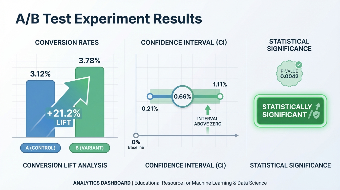
Implementation Hints: For proportions (conversion rates), use a z-test:
p1 = conversions_A / samples_A
p2 = conversions_B / samples_B
p_pooled = (conversions_A + conversions_B) / (samples_A + samples_B)

se = sqrt(p_pooled * (1-p_pooled) * (1/samples_A + 1/samples_B))
z = (p2 - p1) / se

# p-value from standard normal CDF
Confidence interval: (p2 - p1) ± 1.96 * se for 95% CI.
Learning milestones:
- p-value computed correctly → You understand hypothesis testing
- Confidence intervals are correct → You understand uncertainty
- You can explain what p-value actually means → You’ve avoided common misconceptions
The Core Question You Are Answering
How do we distinguish real effects from random noise?
Every day, companies run experiments: does the new button color increase clicks? Does the new algorithm improve engagement? But even with no real difference, random variation will make one group look better. A/B testing gives us the mathematical machinery to answer: “Is this difference real, or could it have happened by chance?” This is the foundation of evidence-based decision making.
Concepts You Must Understand First
Stop and research these before coding:
- Null and Alternative Hypotheses
- What is the null hypothesis in an A/B test? (No difference between groups)
- What is the alternative hypothesis? (There is a difference)
- Why do we try to reject the null rather than prove the alternative?
- Book Reference: “Think Stats” Chapter 7 - Allen Downey
- The p-value
- What does a p-value actually measure?
- Why is p-value NOT the probability that the null hypothesis is true?
- What does “statistically significant at alpha = 0.05” mean?
- Why is the threshold 0.05 arbitrary?
- Book Reference: “Statistics Done Wrong” Chapter 1 - Alex Reinhart
- Type I and Type II Errors
- What is a false positive (Type I error)?
- What is a false negative (Type II error)?
- Why can’t we minimize both simultaneously?
- What is the relationship between alpha and Type I error rate?
- Book Reference: “All of Statistics” Chapter 10 - Larry Wasserman
- The t-test and z-test
- When do you use z-test vs t-test?
- What is the test statistic measuring?
- Why does sample size affect the test statistic?
- What assumptions does the t-test make?
- Book Reference: “Think Stats” Chapter 9 - Allen Downey
- Confidence Intervals
- What does a “95% confidence interval” actually mean?
- How is a confidence interval related to hypothesis testing?
- Why does the interval get narrower with more samples?
- Book Reference: “All of Statistics” Chapter 6 - Larry Wasserman
- Statistical Power and Sample Size
- What is statistical power? (Probability of detecting a real effect)
- Why is 80% power a common target?
- How do you calculate required sample size for a desired power?
- What is the relationship between effect size, sample size, and power?
- Book Reference: “Statistics Done Wrong” Chapter 4 - Alex Reinhart
Questions to Guide Your Design
Before implementing, think through these:
-
Input Format: How will you accept A/B test data? Two lists of outcomes? A CSV with group labels?
-
Test Selection: Will you implement both z-test (for proportions) and t-test (for means)? How will you choose which to use?
-
Two-tailed vs One-tailed: Will you support both? What’s the difference in p-value calculation?
-
Confidence Interval Method: Will you use the normal approximation or exact methods? When might the approximation fail?
-
Sample Size Calculator: How will you implement power analysis? What inputs do you need (baseline rate, minimum detectable effect, power, alpha)?
-
Multiple Testing: What happens when someone runs many A/B tests? How would you handle the multiple comparison problem?
Thinking Exercise
Work through a complete A/B test by hand:
An e-commerce site runs an A/B test on a new checkout button:
- Control (A): 1000 visitors, 50 conversions (5.0% conversion rate)
- Treatment (B): 1000 visitors, 65 conversions (6.5% conversion rate)
Step 1: State the hypotheses
- H0: p_A = p_B (no difference)
- H1: p_A != p_B (there is a difference)
Step 2: Compute the pooled proportion
p_pooled = (50 + 65) / (1000 + 1000) = ?
Step 3: Compute the standard error
SE = sqrt(p_pooled * (1 - p_pooled) * (1/n_A + 1/n_B))
   = sqrt(? * ? * (1/1000 + 1/1000))
   = ?
Step 4: Compute the z-statistic
z = (p_B - p_A) / SE
  = (0.065 - 0.050) / ?
  = ?
Step 5: Find the p-value Using a standard normal table or calculator:
-
For two-tailed test: p-value = 2 * P(Z > z ) = ?
Step 6: Make a decision
- If p-value < 0.05, reject H0
- Is the result statistically significant?
Step 7: Compute confidence interval
CI = (p_B - p_A) +/- 1.96 * SE
   = ? +/- ?
   = [?, ?]
Does this interval include 0? Does that match your hypothesis test conclusion?
The Interview Questions They Will Ask
- “Explain what a p-value is.”
- Expected: The probability of observing results as extreme as ours (or more extreme), assuming the null hypothesis is true. NOT the probability that the null is true.
- “What is the difference between statistical significance and practical significance?”
- Expected: Statistical significance means unlikely due to chance. Practical significance means the effect size matters for business. A tiny effect can be statistically significant with large samples.
- “How do you determine sample size for an A/B test?”
- Expected: Power analysis. Need baseline conversion rate, minimum detectable effect, desired power (usually 80%), and significance level (usually 0.05).
- “What is p-hacking and how do you avoid it?”
- Expected: Testing multiple hypotheses until finding significance, or stopping early when significance is reached. Avoid by pre-registering hypotheses, using correction for multiple comparisons, and fixed sample sizes.
- “What happens if you run 20 A/B tests with no real effects?”
- Expected: At alpha = 0.05, expect 1 false positive on average. This is the multiple testing problem. Use Bonferroni correction or False Discovery Rate methods.
- “Can you reject the null hypothesis with a small sample?”
- Expected: Yes, if the effect is very large. But small samples give wide confidence intervals. Statistical power is low, so you might miss real effects.
- “What’s the difference between a confidence interval and a credible interval?”
- Expected: Confidence interval is frequentist: in repeated experiments, 95% of intervals contain the true value. Credible interval is Bayesian: there’s 95% probability the true value is in this interval.
Hints in Layers
Hint 1: Basic Test Structure For proportion tests, you need: number of successes and total trials for each group. From these, compute sample proportions.
Hint 2: The Z-test for Proportions
def z_test_proportions(successes_a, n_a, successes_b, n_b):
    p_a = successes_a / n_a
    p_b = successes_b / n_b

    # Pooled proportion under null hypothesis
    p_pooled = (successes_a + successes_b) / (n_a + n_b)

    # Standard error
    se = math.sqrt(p_pooled * (1 - p_pooled) * (1/n_a + 1/n_b))

    # Z statistic
    z = (p_b - p_a) / se

    return z
Hint 3: P-value from Z-score
from scipy import stats

# Two-tailed p-value
p_value = 2 * (1 - stats.norm.cdf(abs(z)))

# Or equivalently
p_value = 2 * stats.norm.sf(abs(z))
Hint 4: Confidence Interval
def confidence_interval(p_a, p_b, n_a, n_b, confidence=0.95):
    # Standard error for difference (not pooled)
    se = math.sqrt(p_a*(1-p_a)/n_a + p_b*(1-p_b)/n_b)

    # Z critical value
    z_crit = stats.norm.ppf((1 + confidence) / 2)

    diff = p_b - p_a
    margin = z_crit * se

    return (diff - margin, diff + margin)
Hint 5: Sample Size Calculation
def required_sample_size(baseline, mde, power=0.8, alpha=0.05):
    """
    baseline: current conversion rate (e.g., 0.05)
    mde: minimum detectable effect (relative, e.g., 0.1 for 10% lift)
    """
    p1 = baseline
    p2 = baseline * (1 + mde)

    # Z values
    z_alpha = stats.norm.ppf(1 - alpha/2)
    z_beta = stats.norm.ppf(power)

    # Pooled variance estimate
    p_avg = (p1 + p2) / 2

    n = 2 * ((z_alpha * math.sqrt(2*p_avg*(1-p_avg)) +
              z_beta * math.sqrt(p1*(1-p1) + p2*(1-p2))) ** 2) / (p2 - p1) ** 2

    return math.ceil(n)
Books That Will Help
| Topic | Book | Chapter |
|---|---|---|
| Hypothesis Testing Foundations | “Think Stats” | Chapter 7 - Allen Downey |
| Common Statistical Mistakes | “Statistics Done Wrong” | All Chapters - Alex Reinhart |
| Confidence Intervals | “All of Statistics” | Chapter 6 - Larry Wasserman |
| Power Analysis | “Statistics Done Wrong” | Chapter 4 - Alex Reinhart |
| The t-test in Depth | “Think Stats” | Chapter 9 - Allen Downey |
| Multiple Testing | “All of Statistics” | Chapter 10 - Larry Wasserman |
| Bayesian A/B Testing | “Think Bayes” | Chapter 8 - Allen Downey |
Common Pitfalls and Debugging
Problem 1: “Outputs drift after a few iterations”
- Why: Hidden numerical instability (unscaled features, aggressive step size, or repeated subtraction of nearly equal values).
- Fix: Normalize inputs, reduce step size, and track relative error rather than only absolute error.
- Quick test: Run the same task with two scales of input (for example x and 10x) and compare normalized error curves.
Problem 2: “Results are inconsistent across runs”
- Why: Random seeds, data split randomness, or non-deterministic ordering are uncontrolled.
- Fix: Set seeds, log configuration, and store split indices and hyperparameters with each run.
- Quick test: Re-run three times with the same seed and confirm metrics remain inside a tight tolerance band.
Problem 3: “The project works on the demo case but fails on edge cases”
- Why: Tests only cover happy-path inputs.
- Fix: Add adversarial inputs (empty values, extreme ranges, near-singular matrices, rare classes).
- Quick test: Build an edge-case test matrix and ensure every scenario reports expected behavior.
Definition of Done
- Core functionality works on reference inputs
- Edge cases are tested and documented
- Results are reproducible (seeded and versioned configuration)
- Performance or convergence behavior is measured and explained
- A short retrospective explains what failed first and how you fixed it
Project 16: Markov Chain Text Generator
- File: P16-markov-chain-text-generator.md
- Main Programming Language: Python
- Alternative Programming Languages: C, JavaScript, Rust
- Coolness Level: Level 4: Hardcore Tech Flex
- Business Potential: 2. The “Micro-SaaS / Pro Tool” (Solo-Preneur Potential)
- Difficulty: Level 2: Intermediate (The Developer)
- Knowledge Area: Probability / Markov Chains
- Software or Tool: Text Generator
- Main Book: “Speech and Language Processing” by Jurafsky & Martin
What you’ll build: A text generator that learns from a corpus (e.g., Shakespeare) and generates new text that mimics the style. Uses Markov chains: the next word depends only on the previous n words.
Why it teaches probability: Markov chains are foundational for understanding sequential data and probabilistic models. The “memoryless” property (future depends only on present, not past) simplifies computation while capturing patterns. This leads to HMMs, RNNs, and beyond.
Core challenges you’ll face:
- Building transition probability table → maps to conditional probabilities
- Sampling from probability distribution → maps to weighted random choice
- Varying n-gram size → maps to model complexity trade-offs
- Handling beginning/end of sentences → maps to boundary conditions
- Generating coherent text → maps to capturing language structure
Key Concepts:
- Markov Chains: “All of Statistics” Chapter 21 - Larry Wasserman
- N-gram Models: “Speech and Language Processing” Chapter 3 - Jurafsky & Martin
- Conditional Probability: “Think Bayes” Chapter 2 - Allen Downey
- Language Modeling: “Natural Language Processing” Chapter 4 - Eisenstein
Difficulty: Intermediate Time estimate: 1 week Prerequisites: Basic probability, file handling
Real World Outcome
$ python markov.py train shakespeare.txt --order=2

Training on Shakespeare's complete works...
Vocabulary: 29,066 unique words
Bigram transitions: 287,432

$ python markov.py generate --words=50

Generated text (order-2 Markov chain):
"To be or not to be, that is the question. Whether 'tis nobler
in the mind to suffer the slings and arrows of outrageous fortune,
or to take arms against a sea of troubles and by opposing end them."

$ python markov.py generate --order=1 --words=50

Generated text (order-1, less coherent):
"The to a of and in that is not be for it with as his this
but have from or one all were her they..."

[Shows transition table for common words]
P(next="be" | current="to") = 0.15
P(next="the" | current="to") = 0.12
Implementation Hints:
Build a dictionary: transitions[context] = {word: count, ...}
For bigrams (order-1): context is single previous word. For trigrams (order-2): context is tuple of two previous words.
To generate:
context = start_token
while True:
    candidates = transitions[context]
    next_word = weighted_random_choice(candidates)
    if next_word == end_token:
        break
    output.append(next_word)
    context = update_context(context, next_word)
Higher order = more coherent but less creative (starts copying source).
Learning milestones:
- Generated text is grammatical-ish → You understand transition probabilities
- Higher order = more coherent → You understand model complexity trade-offs
- You see this as a simple language model → You’re ready for RNNs/transformers
The Core Question You Are Answering
“How much of the past do you need to remember to predict the future?”
This is one of the deepest questions in sequence modeling. Markov chains give a precise answer: you only need the last n states. This “memoryless” property seems limiting, but it is remarkably powerful. Language has patterns–“to be” is often followed by “or”–and these patterns are captured by conditional probabilities. The philosophical insight: most sequential data has structure, and that structure can be exploited even with limited memory. Modern transformers use attention to look at ALL previous states, but Markov chains teach you why that is valuable by showing you what is lost when you cannot.
Concepts You Must Understand First
Stop and research these before coding:
-
**Conditional Probability P(A B)** - What does “probability of A given B” actually mean?
- How is it different from P(A and B)?
-
Why does P(next_word current_word) define the whole Markov chain? - Book Reference: “Think Bayes” Chapter 1 - Allen Downey
- The Markov Property (Memorylessness)
- What does it mean that “the future depends only on the present”?
- Why is this assumption both a simplification and a feature?
- How do n-gram models extend this to “n states” of memory?
- Book Reference: “All of Statistics” Chapter 21 - Larry Wasserman
- Transition Probability Matrices
-
How do you represent all P(next current) in a matrix? - What do the rows and columns mean?
- Why must each row sum to 1?
- Book Reference: “Speech and Language Processing” Chapter 3 - Jurafsky & Martin
-
- N-gram Language Models
- What is the difference between unigrams, bigrams, trigrams?
- How does increasing n affect model behavior?
- What is the tradeoff between memory and generalization?
- Book Reference: “Natural Language Processing” Chapter 4 - Eisenstein
- Sampling from Discrete Distributions
- How do you pick a random word according to probabilities?
- What is the weighted random choice algorithm?
- Why is this fundamental to generative models?
- Book Reference: “Grokking Algorithms” Chapter 10 - Aditya Bhargava
Questions to Guide Your Design
Before implementing, think through these:
-
Data structure for transitions: How will you store P(next context) efficiently? A dictionary of dictionaries? What happens when context has not been seen? -
Handling sentence boundaries: How do you know when to start a new sentence? Do you need special START and END tokens?
-
Smoothing unseen transitions: What if your model encounters a context it never saw during training? Should probability be 0, or should you “smooth” it somehow?
-
Order selection: How do you let users choose bigrams vs trigrams vs higher? How does your data structure change?
-
Memory vs creativity tradeoff: With high n, the model starts copying the source verbatim. How do you measure this? What is the “right” n?
- Evaluation: How do you measure if generated text is “good”? Perplexity? Human evaluation?
Thinking Exercise
Before coding, trace through this by hand:
Given this tiny corpus: “the cat sat. the cat ran. the dog sat.”
Build the bigram (order-1) transition table:
P(next | "the") = ?
P(next | "cat") = ?
P(next | "dog") = ?
P(next | "sat") = ?
P(next | "ran") = ?
Now generate text starting from “the”:
-
Look up P(next “the”). What are the options? - Randomly choose according to probabilities
- Repeat until you hit a sentence end
Questions to answer:
-
What is P(“cat” “the”)? What is P(“dog” “the”)? - Why can you not generate “the dog ran” even though all words exist?
- What would happen with a trigram model on this tiny corpus?
The Interview Questions They Will Ask
- “What is the Markov property and why is it useful?”
- Expected answer: Future depends only on present state, not full history. Useful because it makes computation tractable–you only need to track current state.
- “How do Markov chains relate to modern language models like GPT?”
- Expected answer: Markov chains are a simple language model. GPT uses attention to consider ALL previous tokens (not just the last n), with learned representations instead of raw counts.
- “What is the time and space complexity of training an n-gram model?”
- Expected answer: O(total_words) time to scan corpus. Space is O(vocab^n) in worst case but typically sparse–actual unique n-grams seen.
- “How would you handle words not seen during training?”
- Expected answer: Smoothing techniques like Laplace (add-1), Kneser-Ney, or backoff to lower-order models.
- “What is perplexity and how does it relate to Markov chains?”
- Expected answer: Perplexity measures how “surprised” the model is by test data. Lower is better. For Markov chains, perplexity = 2^(cross-entropy).
- “Why do higher-order Markov models eventually just memorize the training data?”
- Expected answer: With high n, each context becomes unique, so there is only one possible next word–the exact word from training. Model loses ability to generalize.
Hints in Layers
Hint 1: Start by just counting. Build a dictionary where keys are contexts (single words for bigrams, tuples for higher) and values are dictionaries mapping next_word to count.
Hint 2: To sample from counts, convert to probabilities by dividing each count by the total for that context. Use random.choices() with weights, or implement weighted random choice yourself.
Hint 3: For sentence boundaries, add special tokens like <START> and <END>. When training, each sentence becomes: <START> word1 word2 ... wordN <END>. When generating, start from <START> and stop when you hit <END>.
Hint 4: For higher-order models (trigrams, etc.), use tuples as dictionary keys: transitions[("the", "cat")] = {"sat": 1, "ran": 1}. The tuple represents the context.
Hint 5: If you want the model to be more “creative,” add temperature scaling: instead of sampling from raw probabilities, raise them to power 1/T and renormalize. T > 1 makes output more random; T < 1 makes it more deterministic.
Books That Will Help
| Topic | Book | Chapter |
|---|---|---|
| Markov Chains Theory | “All of Statistics” by Larry Wasserman | Chapter 21: Markov Chain Monte Carlo |
| N-gram Language Models | “Speech and Language Processing” by Jurafsky & Martin | Chapter 3: N-gram Language Models |
| Conditional Probability | “Think Bayes” by Allen Downey | Chapter 1-2: Probability Basics |
| Smoothing Techniques | “Foundations of Statistical NLP” by Manning & Schutze | Chapter 6: Statistical Estimation |
| Language Model Evaluation | “Natural Language Processing” by Eisenstein | Chapter 6: Language Models |
| Practical Implementation | “Natural Language Processing with Python” by Bird et al. | Chapter 2: Accessing Text |
Part 5: Optimization
Optimization is how machines “learn.” Every ML algorithm boils down to: define a loss function, then minimize it.
Common Pitfalls and Debugging
Problem 1: “Outputs drift after a few iterations”
- Why: Hidden numerical instability (unscaled features, aggressive step size, or repeated subtraction of nearly equal values).
- Fix: Normalize inputs, reduce step size, and track relative error rather than only absolute error.
- Quick test: Run the same task with two scales of input (for example x and 10x) and compare normalized error curves.
Problem 2: “Results are inconsistent across runs”
- Why: Random seeds, data split randomness, or non-deterministic ordering are uncontrolled.
- Fix: Set seeds, log configuration, and store split indices and hyperparameters with each run.
- Quick test: Re-run three times with the same seed and confirm metrics remain inside a tight tolerance band.
Problem 3: “The project works on the demo case but fails on edge cases”
- Why: Tests only cover happy-path inputs.
- Fix: Add adversarial inputs (empty values, extreme ranges, near-singular matrices, rare classes).
- Quick test: Build an edge-case test matrix and ensure every scenario reports expected behavior.
Definition of Done
- Core functionality works on reference inputs
- Edge cases are tested and documented
- Results are reproducible (seeded and versioned configuration)
- Performance or convergence behavior is measured and explained
- A short retrospective explains what failed first and how you fixed it
Project 17: Linear Regression from Scratch
- File: P17-linear-regression-from-scratch.md
- Main Programming Language: Python
- Alternative Programming Languages: C, Julia, Rust
- Coolness Level: Level 3: Genuinely Clever
- Business Potential: 1. The “Resume Gold” (Educational/Personal Brand)
- Difficulty: Level 2: Intermediate (The Developer)
- Knowledge Area: Regression / Optimization
- Software or Tool: Linear Regression
- Main Book: “Hands-On Machine Learning” by Aurélien Géron
What you’ll build: Linear regression implemented two ways: (1) analytically using the normal equation, and (2) iteratively using gradient descent. Compare their performance and understand when to use each.
Why it teaches optimization: Linear regression is the “hello world” of ML optimization. The normal equation shows the closed-form solution (linear algebra). Gradient descent shows the iterative approach (calculus). Understanding both is foundational.
Core challenges you’ll face:
- Implementing normal equation → maps to (X^T X)^{-1} X^T y
- Implementing gradient descent → maps to iterative optimization
- Mean squared error loss → maps to loss functions
- Feature scaling → maps to preprocessing for optimization
- Comparing analytical vs iterative → maps to algorithm trade-offs
Key Concepts:
- Linear Regression: “Hands-On Machine Learning” Chapter 4 - Aurélien Géron
- Normal Equation: “Machine Learning” (Coursera) Week 2 - Andrew Ng
- Gradient Descent for Regression: “Deep Learning” Chapter 4 - Goodfellow et al.
- Feature Scaling: “Data Science for Business” Chapter 4 - Provost & Fawcett
Difficulty: Intermediate Time estimate: 1 week Prerequisites: Project 4 (matrices), Project 9 (gradient descent)
Real World Outcome
$ python linear_regression.py housing.csv --target=price

Loading data: 500 samples, 5 features

Method 1: Normal Equation (analytical)
  Computation time: 0.003s
  Weights: [intercept=5.2, sqft=0.0012, bedrooms=2.3, ...]

Method 2: Gradient Descent (iterative)
  Learning rate: 0.01
  Iterations: 1000
  Computation time: 0.15s
  Final loss: 0.0234
  Weights: [intercept=5.1, sqft=0.0012, bedrooms=2.4, ...]

[Plot: Gradient descent loss decreasing over iterations]
[Plot: Predicted vs actual prices scatter plot]

Test set performance:
  R² Score: 0.87
  RMSE: $45,230

$ python linear_regression.py --predict "sqft=2000, bedrooms=3, ..."
Predicted price: $425,000
Implementation Hints: Normal equation:
# X is (n_samples, n_features+1) with column of 1s for intercept
# y is (n_samples,)
w = np.linalg.inv(X.T @ X) @ X.T @ y
Gradient descent:
w = np.zeros(n_features + 1)
for _ in range(iterations):
    predictions = X @ w
    error = predictions - y
    gradient = (2/n_samples) * X.T @ error
    w = w - learning_rate * gradient
Feature scaling (important for gradient descent!):
X_scaled = (X - X.mean(axis=0)) / X.std(axis=0)
Learning milestones:
- Both methods give same answer → You understand they solve the same problem
- Gradient descent needs feature scaling → You understand optimization dynamics
- You know when to use each → Normal equation for small data, GD for large
The Core Question You Are Answering
“When can we solve a problem exactly, and when must we iterate toward the answer?”
Linear regression presents you with a fundamental dichotomy in optimization. The normal equation gives you the exact answer in one matrix computation–no iteration, no learning rate, no convergence worries. But it requires inverting a matrix, which becomes prohibitively expensive for large datasets. Gradient descent trades exactness for scalability–you get arbitrarily close to the answer through iteration, and it works even when you have millions of features. This tension between closed-form solutions and iterative methods pervades all of machine learning. Understanding when each approach applies–and why–is essential.
Concepts You Must Understand First
Stop and research these before coding:
- Mean Squared Error (MSE) Loss
- Why do we square the errors instead of using absolute values?
- What is the geometric interpretation of MSE?
- How does MSE relate to the assumption that errors are normally distributed?
- Book Reference: “Hands-On Machine Learning” Chapter 4 - Aurelien Geron
- The Normal Equation Derivation
- What does it mean to “set the gradient to zero”?
- Why does the solution involve (X^T X)^(-1)?
- When is X^T X invertible? When is it not?
- Book Reference: “Machine Learning” (Coursera) Week 2 - Andrew Ng
- Matrix Inversion Complexity
- What is the time complexity of inverting an n x n matrix?
- Why does this become prohibitive for large feature counts?
- What is the Moore-Penrose pseudoinverse and when do you need it?
- Book Reference: “Linear Algebra Done Right” Chapter 3 - Sheldon Axler
- Gradient Descent Mechanics
- Why is the gradient of MSE equal to 2X^T(Xw - y)/n?
- What does the learning rate control, geometrically?
- Why does feature scaling help gradient descent converge faster?
- Book Reference: “Deep Learning” Chapter 4 - Goodfellow et al.
- R-squared Score
- What does R^2 = 0.87 actually mean in terms of explained variance?
- How is R^2 related to MSE?
- Why can R^2 be negative on test data?
- Book Reference: “Data Science for Business” Chapter 4 - Provost & Fawcett
- The Bias Term (Intercept)
- Why do we add a column of ones to X?
- What happens if you forget the bias term?
- How does centering data relate to the intercept?
- Book Reference: “Hands-On Machine Learning” Chapter 4 - Aurelien Geron
Questions to Guide Your Design
Before implementing, think through these:
-
Data augmentation for bias: How do you add the column of ones to X to handle the intercept term? Do you add it as the first or last column?
-
Feature scaling strategy: Will you standardize (mean=0, std=1) or normalize (min=0, max=1)? Why does gradient descent care but normal equation does not?
-
Normal equation numerical stability: What happens when X^T X is nearly singular? How do you detect and handle this?
-
Gradient descent stopping criteria: When do you stop iterating? Fixed epochs? Convergence threshold? Both?
-
Batch vs stochastic vs mini-batch: Will you compute the gradient on all data (batch) or subsets? How does this affect convergence?
-
Comparison methodology: How will you verify that both methods give the same answer? What tolerance is acceptable?
Thinking Exercise
Work through this 2D example by hand:
Data points:
X = [[1], [2], [3]]  (one feature)
y = [2, 4, 5]        (targets)
Step 1: Add bias column
X_aug = [[1, 1], [1, 2], [1, 3]] (column of ones added)
Step 2: Normal equation
X^T X = ?
(X^T X)^(-1) = ?
X^T y = ?
w = (X^T X)^(-1) X^T y = ?
Step 3: Verify with gradient descent Start with w = [0, 0], learning_rate = 0.1
Iteration 1:
  predictions = X_aug @ w = ?
  errors = predictions - y = ?
  gradient = (2/3) * X_aug^T @ errors = ?
  w_new = w - 0.1 * gradient = ?
After many iterations, w should converge to the same answer as the normal equation.
The Interview Questions They Will Ask
- “Derive the normal equation for linear regression.”
- Expected answer: Start with MSE loss, take gradient with respect to w, set to zero, solve for w to get w = (X^T X)^(-1) X^T y.
- “When would you choose gradient descent over the normal equation?”
- Expected answer: Large number of features (n > 10,000), need online learning, memory constraints, or when X^T X is ill-conditioned.
- “What is the computational complexity of both approaches?”
- Expected answer: Normal equation is O(n^3) for matrix inversion where n is number of features. Gradient descent is O(m * n * k) where m is samples, k is iterations.
- “Why must you scale features for gradient descent but not for the normal equation?”
- Expected answer: Unscaled features create elongated contours in the loss surface, causing gradient descent to oscillate. Normal equation algebraically solves regardless of scale.
- “What is the difference between R^2 on training data vs test data?”
- Expected answer: Training R^2 can only increase with more features (overfitting). Test R^2 measures generalization and can decrease or go negative if model is overfit.
- “How would you extend this to polynomial regression?”
- Expected answer: Create polynomial features (x^2, x^3, x1*x2, etc.) and apply the same linear regression. Model is still “linear in parameters.”
- “What is regularization and why might you need it?”
- Expected answer: Adding a penalty term (L1 or L2) to the loss prevents large weights and reduces overfitting. L2 regularization has a closed-form solution: w = (X^T X + lambda*I)^(-1) X^T y.
Hints in Layers
Hint 1: Start simple. Implement the normal equation first since it is just matrix operations:
X_aug = np.column_stack([np.ones(len(X)), X])
w = np.linalg.inv(X_aug.T @ X_aug) @ X_aug.T @ y
Hint 2: For gradient descent, the key formula is:
gradient = (2/n_samples) * X_aug.T @ (X_aug @ w - y)
w = w - learning_rate * gradient
Hint 3: Feature scaling for gradient descent:
X_mean, X_std = X.mean(axis=0), X.std(axis=0)
X_scaled = (X - X_mean) / X_std
# Remember to transform test data with training statistics!
Hint 4: For numerical stability with the normal equation, use np.linalg.pinv (pseudoinverse) or add a small ridge term:
w = np.linalg.inv(X.T @ X + 1e-8 * np.eye(n_features)) @ X.T @ y
Hint 5: To compute R^2:
ss_res = np.sum((y - predictions)**2)
ss_tot = np.sum((y - y.mean())**2)
r2 = 1 - ss_res / ss_tot
Books That Will Help
| Topic | Book | Chapter |
|---|---|---|
| Linear Regression Theory | “Hands-On Machine Learning” by Aurelien Geron | Chapter 4: Training Models |
| Normal Equation Derivation | “Machine Learning” (Coursera) by Andrew Ng | Week 2: Linear Regression |
| Gradient Descent Intuition | “Deep Learning” by Goodfellow et al. | Chapter 4: Numerical Computation |
| Matrix Calculus | “Math for Programmers” by Paul Orland | Chapter 12: Multivariable Calculus |
| Feature Scaling | “Data Science for Business” by Provost & Fawcett | Chapter 4: Modeling |
| Regularization | “The Elements of Statistical Learning” by Hastie et al. | Chapter 3: Linear Regression |
Common Pitfalls and Debugging
Problem 1: “Outputs drift after a few iterations”
- Why: Hidden numerical instability (unscaled features, aggressive step size, or repeated subtraction of nearly equal values).
- Fix: Normalize inputs, reduce step size, and track relative error rather than only absolute error.
- Quick test: Run the same task with two scales of input (for example x and 10x) and compare normalized error curves.
Problem 2: “Results are inconsistent across runs”
- Why: Random seeds, data split randomness, or non-deterministic ordering are uncontrolled.
- Fix: Set seeds, log configuration, and store split indices and hyperparameters with each run.
- Quick test: Re-run three times with the same seed and confirm metrics remain inside a tight tolerance band.
Problem 3: “The project works on the demo case but fails on edge cases”
- Why: Tests only cover happy-path inputs.
- Fix: Add adversarial inputs (empty values, extreme ranges, near-singular matrices, rare classes).
- Quick test: Build an edge-case test matrix and ensure every scenario reports expected behavior.
Definition of Done
- Core functionality works on reference inputs
- Edge cases are tested and documented
- Results are reproducible (seeded and versioned configuration)
- Performance or convergence behavior is measured and explained
- A short retrospective explains what failed first and how you fixed it
Project 18: Logistic Regression Classifier
- File: P18-logistic-regression-classifier.md
- Main Programming Language: Python
- Alternative Programming Languages: C, Julia, Rust
- Coolness Level: Level 3: Genuinely Clever
- Business Potential: 2. The “Micro-SaaS / Pro Tool” (Solo-Preneur Potential)
- Difficulty: Level 3: Advanced (The Engineer)
- Knowledge Area: Classification / Optimization
- Software or Tool: Logistic Classifier
- Main Book: “Hands-On Machine Learning” by Aurélien Géron
What you’ll build: A binary classifier using logistic regression with gradient descent. Train on labeled data, learn the decision boundary, and visualize the sigmoid probability outputs.
Why it teaches optimization: Logistic regression bridges linear algebra, calculus, and probability. The sigmoid function squashes linear output to [0,1]. Cross-entropy loss measures probability error. Gradient descent finds optimal weights. It’s the perfect “next step” from linear regression.
Core challenges you’ll face:
- Sigmoid activation function → maps to probability output
- Binary cross-entropy loss → maps to negative log likelihood
- Gradient computation → maps to ∂L/∂w = (σ(z) - y) · x
- Decision boundary visualization → maps to linear separator in feature space
- Regularization → maps to preventing overfitting
Key Concepts:
- Logistic Regression: “Hands-On Machine Learning” Chapter 4 - Aurélien Géron
- Cross-Entropy Loss: “Deep Learning” Chapter 3 - Goodfellow et al.
- Sigmoid Function: “Neural Networks and Deep Learning” Chapter 1 - Michael Nielsen
- Regularization: “Machine Learning” (Coursera) Week 3 - Andrew Ng
Difficulty: Advanced Time estimate: 1-2 weeks Prerequisites: Project 11, Project 17
Real World Outcome
$ python logistic.py train iris_binary.csv

Training logistic regression on Iris dataset (setosa vs non-setosa)
Features: sepal_length, sepal_width
Samples: 150 (50 setosa, 100 non-setosa)

Training...
Epoch 100:  Loss = 0.423, Accuracy = 92%
Epoch 500:  Loss = 0.187, Accuracy = 97%
Epoch 1000: Loss = 0.124, Accuracy = 99%

Learned weights:
  w_sepal_length = -2.34
  w_sepal_width  =  4.12
  bias           = -1.56

Decision boundary: sepal_width = 0.57 * sepal_length + 0.38

[2D plot: points colored by class, linear decision boundary shown]
[Probability surface: darker = more confident]

$ python logistic.py predict "sepal_length=5.0, sepal_width=3.5"
P(setosa) = 0.94
Classification: setosa (high confidence)
Implementation Hints: Forward pass:
z = X @ w + b
prob = 1 / (1 + np.exp(-z))  # sigmoid
Cross-entropy loss:
loss = -np.mean(y * np.log(prob + 1e-10) + (1-y) * np.log(1-prob + 1e-10))
Gradient (beautifully simple!):
gradient_w = X.T @ (prob - y) / n_samples
gradient_b = np.mean(prob - y)
The gradient has the same form as linear regression—this is not a coincidence!
Learning milestones:
- Classifier achieves high accuracy → You understand logistic regression
- Decision boundary is correct → You understand linear separability
- Probability outputs are calibrated → You understand probabilistic classification
The Core Question You Are Answering
“How do you turn a line into a decision?”
Linear regression predicts continuous values, but what if you need to predict yes or no, spam or not spam, cat or dog? You cannot just use a line because lines extend to infinity in both directions. The insight is to “squash” the linear output through a sigmoid function, transforming any real number into a probability between 0 and 1. This simple idea–applying a nonlinear transformation to a linear model–is the foundation of neural networks. By building logistic regression, you understand the key transition from regression to classification, from predicting “how much” to predicting “which one.”
Concepts You Must Understand First
Stop and research these before coding:
- The Sigmoid Function
- What is the formula for sigmoid: 1 / (1 + exp(-z))?
- Why does it squash all real numbers to (0, 1)?
- What is the derivative of sigmoid? Why is it so elegant?
- Book Reference: “Neural Networks and Deep Learning” Chapter 1 - Michael Nielsen
- Binary Cross-Entropy Loss
- Why do we use -ylog(p) - (1-y)log(1-p) instead of squared error?
- What happens to the loss when prediction is confident and wrong?
- How does this relate to maximum likelihood estimation?
- Book Reference: “Deep Learning” Chapter 3 - Goodfellow et al.
- Decision Boundaries
- What is the equation of the decision boundary for logistic regression?
- Why is the boundary always linear (a hyperplane)?
- What does it mean for data to be “linearly separable”?
- Book Reference: “Hands-On Machine Learning” Chapter 4 - Aurelien Geron
- Gradient of Cross-Entropy Loss
- Why does the gradient simplify to (prediction - label) * input?
- How is this similar to the gradient for linear regression?
- What makes this mathematical coincidence significant?
- Book Reference: “Machine Learning” (Coursera) Week 3 - Andrew Ng
- Regularization (L1 and L2)
- What is the difference between L1 (lasso) and L2 (ridge) regularization?
- Why does regularization prevent overfitting?
- How does it affect the decision boundary?
- Book Reference: “The Elements of Statistical Learning” Chapter 3 - Hastie et al.
- Probability Calibration
- What does it mean for predicted probabilities to be “calibrated”?
- How do you check if your model’s 80% predictions are actually correct 80% of the time?
- Why is calibration important for real applications?
- Book Reference: “Probabilistic Machine Learning” Chapter 5 - Kevin Murphy
Questions to Guide Your Design
Before implementing, think through these:
-
Numerical stability: What happens when exp(-z) overflows? How do you handle very large or very small values of z?
-
Learning rate selection: How do you choose an appropriate learning rate? What symptoms indicate it is too high or too low?
-
Convergence criteria: When do you stop training? Fixed epochs? Loss threshold? Validation accuracy plateau?
-
Handling imbalanced data: What if 95% of your data belongs to one class? How does this affect training?
-
Multiclass extension: How would you extend binary logistic regression to handle more than two classes?
-
Feature importance: After training, how can you interpret which features matter most for the classification?
Thinking Exercise
Work through sigmoid and its derivative by hand:
- Compute sigmoid for these values:
- z = 0: sigmoid(0) = 1/(1+e^0) = 1/(1+1) = 0.5
- z = 10: sigmoid(10) = 1/(1+e^(-10)) is approximately 0.99995
- z = -10: sigmoid(-10) is approximately 0.00005
- Prove that the derivative of sigmoid is sigmoid(z) * (1 - sigmoid(z)):
- Let s = 1/(1+e^(-z))
- ds/dz = … (work through the calculus)
- Verify gradient descent update:
Given one data point: x = [1, 2], y = 1 (positive class), current weights w = [0.1, 0.2]
- z = w^T x = 0.11 + 0.22 = 0.5
- p = sigmoid(0.5) is approximately 0.622
- loss = -1log(0.622) - 0log(0.378) is approximately 0.475
- gradient = (p - y) * x = (0.622 - 1) * [1, 2] = [-0.378, -0.756]
- new_w = [0.1, 0.2] - 0.1 * [-0.378, -0.756] = [0.138, 0.276]
Notice how the weights moved in the direction that makes the prediction closer to 1!
The Interview Questions They Will Ask
- “Explain the intuition behind logistic regression.”
- Expected answer: It is linear regression followed by a sigmoid function. The linear part creates a weighted sum, sigmoid converts it to probability, and we minimize cross-entropy loss.
- “Why do we use cross-entropy loss instead of MSE for classification?”
- Expected answer: Cross-entropy has stronger gradients when predictions are wrong (log(small number) is very negative). MSE gradients vanish near 0 and 1 due to sigmoid saturation.
- “What is the equation of the decision boundary for logistic regression?”
- Expected answer: w^T x + b = 0, which is a hyperplane. Points above the hyperplane are classified as positive (sigmoid > 0.5).
- “How would you handle a dataset where one class has 100x more samples?”
- Expected answer: Class weights, oversampling minority class (SMOTE), undersampling majority, or adjusting the decision threshold.
- “What happens if your features are linearly dependent?”
- Expected answer: The model still trains, but weights are not unique (infinitely many solutions). Regularization helps by preferring smaller weights.
- “How do you interpret the coefficients of a logistic regression model?”
- Expected answer: exp(w_i) is the odds ratio–how much the odds multiply when feature i increases by 1, holding other features constant.
- “When would logistic regression fail compared to more complex models?”
- Expected answer: When the true decision boundary is nonlinear. Logistic regression can only draw straight lines (hyperplanes).
Hints in Layers
Hint 1: The sigmoid function is your foundation:
def sigmoid(z):
    return 1 / (1 + np.exp(-z))
But beware: large negative z causes overflow. Use np.clip(z, -500, 500) for stability.
Hint 2: Cross-entropy loss with numerical stability:
def cross_entropy(y_true, y_pred):
    epsilon = 1e-15  # Prevent log(0)
    y_pred = np.clip(y_pred, epsilon, 1 - epsilon)
    return -np.mean(y_true * np.log(y_pred) + (1 - y_true) * np.log(1 - y_pred))
Hint 3: The gradient is beautifully simple:
predictions = sigmoid(X @ w + b)
gradient_w = (1/n) * X.T @ (predictions - y)
gradient_b = np.mean(predictions - y)
Hint 4: For the decision boundary visualization (2D features):
# Decision boundary: w1*x1 + w2*x2 + b = 0
# Solve for x2: x2 = -(w1*x1 + b) / w2
x1_range = np.linspace(X[:, 0].min(), X[:, 0].max(), 100)
x2_boundary = -(w[0] * x1_range + b) / w[1]
plt.plot(x1_range, x2_boundary, 'k--', label='Decision Boundary')
Hint 5: Add L2 regularization:
# Regularization term: lambda * ||w||^2 / 2
# Add to loss: loss + lambda * np.sum(w**2) / 2
# Add to gradient: gradient_w + lambda * w
Books That Will Help
| Topic | Book | Chapter |
|---|---|---|
| Logistic Regression Theory | “Hands-On Machine Learning” by Aurelien Geron | Chapter 4: Training Models |
| Cross-Entropy and Maximum Likelihood | “Deep Learning” by Goodfellow et al. | Chapter 3: Probability |
| Sigmoid and Activation Functions | “Neural Networks and Deep Learning” by Michael Nielsen | Chapter 1: Using Neural Nets |
| Regularization | “The Elements of Statistical Learning” by Hastie et al. | Chapter 3: Linear Methods |
| Gradient Descent for Classification | “Machine Learning” (Coursera) by Andrew Ng | Week 3: Logistic Regression |
| Probability Calibration | “Probabilistic Machine Learning” by Kevin Murphy | Chapter 5: Decision Theory |
Common Pitfalls and Debugging
Problem 1: “Outputs drift after a few iterations”
- Why: Hidden numerical instability (unscaled features, aggressive step size, or repeated subtraction of nearly equal values).
- Fix: Normalize inputs, reduce step size, and track relative error rather than only absolute error.
- Quick test: Run the same task with two scales of input (for example x and 10x) and compare normalized error curves.
Problem 2: “Results are inconsistent across runs”
- Why: Random seeds, data split randomness, or non-deterministic ordering are uncontrolled.
- Fix: Set seeds, log configuration, and store split indices and hyperparameters with each run.
- Quick test: Re-run three times with the same seed and confirm metrics remain inside a tight tolerance band.
Problem 3: “The project works on the demo case but fails on edge cases”
- Why: Tests only cover happy-path inputs.
- Fix: Add adversarial inputs (empty values, extreme ranges, near-singular matrices, rare classes).
- Quick test: Build an edge-case test matrix and ensure every scenario reports expected behavior.
Definition of Done
- Core functionality works on reference inputs
- Edge cases are tested and documented
- Results are reproducible (seeded and versioned configuration)
- Performance or convergence behavior is measured and explained
- A short retrospective explains what failed first and how you fixed it
Project 19: Neural Network from First Principles
- File: P19-neural-network-from-first-principles.md
- Main Programming Language: Python
- Alternative Programming Languages: C, Julia, Rust
- Coolness Level: Level 5: Pure Magic (Super Cool)
- Business Potential: 1. The “Resume Gold” (Educational/Personal Brand)
- Difficulty: Level 4: Expert (The Systems Architect)
- Knowledge Area: Deep Learning / Optimization
- Software or Tool: Neural Network
- Main Book: “Neural Networks and Deep Learning” by Michael Nielsen
What you’ll build: A multi-layer neural network that learns to classify handwritten digits (MNIST). Implement forward pass, backpropagation, and training loop from scratch—no TensorFlow, no PyTorch, just NumPy.
Why it teaches optimization: This is the culmination of everything. Matrix multiplication (linear algebra) for forward pass. Chain rule (calculus) for backpropagation. Probability (softmax/cross-entropy) for output. Gradient descent for learning. Building this from scratch demystifies deep learning.
Core challenges you’ll face:
- Multi-layer forward pass → maps to matrix multiplication chains
- Backpropagation through layers → maps to chain rule in depth
- Activation functions (ReLU, sigmoid) → maps to non-linearity
- Softmax for multi-class output → maps to probability distribution
- Mini-batch gradient descent → maps to stochastic optimization
Key Concepts:
- Backpropagation: “Neural Networks and Deep Learning” Chapter 2 - Michael Nielsen
- Softmax and Cross-Entropy: “Deep Learning” Chapter 6 - Goodfellow et al.
- Weight Initialization: “Hands-On Machine Learning” Chapter 11 - Aurélien Géron
- Mini-batch Gradient Descent: “Deep Learning” Chapter 8 - Goodfellow et al.
Difficulty: Expert Time estimate: 3-4 weeks Prerequisites: All previous projects, especially 11, 17, 18
Real World Outcome
$ python neural_net.py mnist/

Loading MNIST dataset...
  Training: 60,000 images
  Test: 10,000 images

Network architecture: 784 → 128 → 64 → 10
  Layer 1: 784 inputs × 128 outputs = 100,352 weights
  Layer 2: 128 × 64 = 8,192 weights
  Layer 3: 64 × 10 = 640 weights
  Total: 109,184 trainable parameters

Training with mini-batch gradient descent (batch_size=32, lr=0.01)

Epoch 1/10:  Loss = 0.823, Accuracy = 78.2%
Epoch 2/10:  Loss = 0.412, Accuracy = 89.1%
Epoch 5/10:  Loss = 0.187, Accuracy = 94.6%
Epoch 10/10: Loss = 0.098, Accuracy = 97.2%

Test set accuracy: 96.8%

[Confusion matrix showing per-digit accuracy]
[Visualization: some misclassified examples with predictions]

$ python neural_net.py predict digit.png
[Shows image]
Prediction: 7 (confidence: 98.3%)
Probabilities: [0.001, 0.002, 0.005, 0.001, 0.002, 0.001, 0.001, 0.983, 0.002, 0.002]
Implementation Hints: Forward pass for layer l:
z[l] = a[l-1] @ W[l] + b[l]
a[l] = activation(z[l])  # ReLU or sigmoid
Backward pass (chain rule!):
# Output layer (with softmax + cross-entropy)
delta[L] = a[L] - y_one_hot  # Beautifully simple!

# Hidden layers
delta[l] = (delta[l+1] @ W[l+1].T) * activation_derivative(z[l])

# Gradients
dW[l] = a[l-1].T @ delta[l]
db[l] = delta[l].sum(axis=0)
This is the mathematical heart of deep learning. Every framework automates this, but you’ll have built it by hand.
Learning milestones:
- Network trains and loss decreases → You understand forward/backward pass
- Accuracy exceeds 95% → You’ve built a working deep learning system
- You can explain backpropagation step-by-step → You’ve internalized the chain rule
The Core Question You Are Answering
“How does a pile of linear algebra and calculus learn to see?”
A neural network is nothing more than alternating linear transformations (matrix multiplications) and nonlinear activations (ReLU, sigmoid). Yet when you stack them together and train with gradient descent, something remarkable happens: the network learns to recognize handwritten digits, or faces, or speech. How? The magic is backpropagation–the chain rule applied systematically to compute how every single weight affects the final loss. By building this from scratch, you will understand that there is no magic at all. Just matrices, derivatives, and the patient accumulation of tiny gradient steps toward a solution.
Concepts You Must Understand First
Stop and research these before coding:
- The Multi-Layer Perceptron Architecture
- What is a “layer” in a neural network?
- How does information flow from input through hidden layers to output?
- What is the role of weights vs biases at each layer?
- Book Reference: “Neural Networks and Deep Learning” Chapter 1 - Michael Nielsen
- Activation Functions (ReLU, Sigmoid, Softmax)
- Why do we need nonlinear activation functions?
- What is the difference between ReLU(z) = max(0, z) and sigmoid?
- When do you use softmax (output layer) vs ReLU (hidden layers)?
- Book Reference: “Deep Learning” Chapter 6 - Goodfellow et al.
- Forward Pass as Matrix Chain Multiplication
- How do you compute the output of a layer: a = activation(W @ x + b)?
- What are the dimensions of W if input is n-dimensional and output is m-dimensional?
- How do you “chain” layers together?
- Book Reference: “Hands-On Machine Learning” Chapter 10 - Aurelien Geron
- Backpropagation (Chain Rule in Depth)
- What is the chain rule: d(f(g(x)))/dx = f’(g(x)) * g’(x)?
- How do you propagate gradients backward through layers?
- Why do you need to cache values from the forward pass?
- Book Reference: “Neural Networks and Deep Learning” Chapter 2 - Michael Nielsen
- Softmax and Cross-Entropy for Multi-Class
- What is softmax: exp(z_i) / sum(exp(z_j))?
- Why is softmax + cross-entropy elegant (gradient = output - target)?
- What is the “log-sum-exp” trick for numerical stability?
- Book Reference: “Deep Learning” Chapter 6 - Goodfellow et al.
- Weight Initialization
- Why do you not initialize all weights to zero?
- What is Xavier/Glorot initialization? What about He initialization?
- How does initialization affect training speed and convergence?
- Book Reference: “Hands-On Machine Learning” Chapter 11 - Aurelien Geron
- Mini-Batch Gradient Descent
- Why use mini-batches instead of all data (batch) or one sample (stochastic)?
- How does batch size affect training dynamics?
- What is an “epoch” in this context?
- Book Reference: “Deep Learning” Chapter 8 - Goodfellow et al.
Questions to Guide Your Design
Before implementing, think through these:
-
Data representation: How will you represent the MNIST images? Flatten to 784-dimensional vectors? Normalize pixel values?
-
Layer abstraction: Will you create a Layer class, or just use functions? How do you store weights and gradients?
-
Forward pass caching: What values do you need to save during forward pass for use in backward pass?
-
Gradient accumulation: In mini-batch training, how do you accumulate gradients across samples before updating weights?
-
Numerical stability: Where might you encounter overflow or underflow? (Hint: softmax, cross-entropy)
-
Training monitoring: How will you track loss and accuracy during training? When do you evaluate on the test set?
Thinking Exercise
Trace backpropagation through a tiny network by hand:
Consider a 2-layer network: Input (2) -> Hidden (2) -> Output (1)
- Input: x = [1, 2]
- Weights layer 1: W1 = [[0.1, 0.2], [0.3, 0.4]], b1 = [0.1, 0.1]
- Weights layer 2: W2 = [[0.5], [0.6]], b2 = [0.1]
- Activation: ReLU for hidden, sigmoid for output
- Target: y = 1
Forward pass:
z1 = W1 @ x + b1 = [[0.1, 0.2], [0.3, 0.4]] @ [1, 2] + [0.1, 0.1] = [0.6, 1.2]
a1 = ReLU(z1) = [0.6, 1.2]
z2 = W2.T @ a1 + b2 = [0.5, 0.6] @ [0.6, 1.2] + 0.1 = 0.5*0.6 + 0.6*1.2 + 0.1 = 1.12
a2 = sigmoid(1.12) = 0.754
Loss = -log(0.754) = 0.282
Backward pass:
dL/da2 = -1/a2 = -1.326  (gradient of cross-entropy w.r.t. prediction)
da2/dz2 = a2*(1-a2) = 0.754 * 0.246 = 0.186  (sigmoid derivative)
dL/dz2 = dL/da2 * da2/dz2 = -1.326 * 0.186 = -0.247
  (or use combined: dL/dz2 = a2 - y = 0.754 - 1 = -0.246)

dL/dW2 = a1 * dL/dz2 = [0.6, 1.2] * (-0.246) = [-0.148, -0.295]
dL/db2 = dL/dz2 = -0.246

dL/da1 = W2 * dL/dz2 = [0.5, 0.6] * (-0.246) = [-0.123, -0.148]
da1/dz1 = [1, 1]  (ReLU derivative, both positive)
dL/dz1 = [-0.123, -0.148]

dL/dW1 = outer(dL/dz1, x) = ... (exercise for you)
dL/db1 = dL/dz1 = [-0.123, -0.148]
The Interview Questions They Will Ask
- “Explain backpropagation in your own words.”
- Expected answer: Backpropagation applies the chain rule to compute how much each weight contributes to the loss. We propagate gradients backward from the output, multiplying by local derivatives at each layer.
- “Why do we need activation functions? What happens without them?”
- Expected answer: Without nonlinear activations, the entire network collapses to a single linear transformation. A stack of linear functions is just one linear function.
- “What is the vanishing gradient problem and how do you address it?”
- Expected answer: Gradients shrink as they propagate through many layers (especially with sigmoid). Solutions: ReLU activation, skip connections (ResNet), batch normalization.
- “Why is mini-batch gradient descent preferred over batch or stochastic?”
- Expected answer: Mini-batch balances computational efficiency (parallel processing) with gradient noise (helps escape local minima). Batch is slow; stochastic is noisy.
- “How do you initialize the weights of a neural network?”
- Expected answer: Xavier/Glorot for sigmoid/tanh (variance = 1/n_in), He for ReLU (variance = 2/n_in). Zero initialization breaks symmetry and prevents learning.
- “What is the difference between epoch, batch, and iteration?”
- Expected answer: Epoch = one pass through all training data. Batch = subset of data for one gradient update. Iteration = one gradient update step.
- “How would you debug a neural network that is not learning?”
- Expected answer: Check: loss decreasing? gradients flowing (not zero or exploding)? learning rate appropriate? data correctly preprocessed? architecture reasonable? overfitting a tiny batch first?
Hints in Layers
Hint 1: Structure your forward pass to cache everything needed for backward:
def forward(X, weights):
    cache = {'input': X}
    A = X
    for i, (W, b) in enumerate(weights):
        Z = A @ W + b
        cache[f'Z{i}'] = Z
        A = relu(Z) if i < len(weights)-1 else softmax(Z)
        cache[f'A{i}'] = A
    return A, cache
Hint 2: The backward pass mirrors the forward:
def backward(y_true, cache, weights):
    grads = []
    m = y_true.shape[0]
    dA = cache['A_last'] - y_true  # softmax + cross-entropy combined

    for i in reversed(range(len(weights))):
        dZ = dA * relu_derivative(cache[f'Z{i}']) if i < len(weights)-1 else dA
        dW = cache[f'A{i-1}'].T @ dZ / m
        db = np.sum(dZ, axis=0) / m
        grads.append((dW, db))
        dA = dZ @ weights[i][0].T

    return list(reversed(grads))
Hint 3: Softmax with numerical stability:
def softmax(z):
    exp_z = np.exp(z - np.max(z, axis=1, keepdims=True))  # subtract max
    return exp_z / np.sum(exp_z, axis=1, keepdims=True)
Hint 4: He initialization for ReLU networks:
W = np.random.randn(n_in, n_out) * np.sqrt(2.0 / n_in)
b = np.zeros(n_out)
Hint 5: Training loop structure:
for epoch in range(epochs):
    for batch_start in range(0, len(X_train), batch_size):
        X_batch = X_train[batch_start:batch_start+batch_size]
        y_batch = y_train[batch_start:batch_start+batch_size]

        output, cache = forward(X_batch, weights)
        grads = backward(y_batch, cache, weights)

        for i, (dW, db) in enumerate(grads):
            weights[i][0] -= learning_rate * dW
            weights[i][1] -= learning_rate * db
Books That Will Help
| Topic | Book | Chapter |
|---|---|---|
| Neural Network Fundamentals | “Neural Networks and Deep Learning” by Michael Nielsen | Chapters 1-2: Networks, Backpropagation |
| Backpropagation Math | “Deep Learning” by Goodfellow et al. | Chapter 6: Deep Feedforward Networks |
| Softmax and Cross-Entropy | “Deep Learning” by Goodfellow et al. | Chapter 6.2: Output Units |
| Weight Initialization | “Hands-On Machine Learning” by Aurelien Geron | Chapter 11: Training Deep Networks |
| Mini-Batch Optimization | “Deep Learning” by Goodfellow et al. | Chapter 8: Optimization |
| Practical Implementation | “Make Your Own Neural Network” by Tariq Rashid | Full book: step-by-step |
Common Pitfalls and Debugging
Problem 1: “Outputs drift after a few iterations”
- Why: Hidden numerical instability (unscaled features, aggressive step size, or repeated subtraction of nearly equal values).
- Fix: Normalize inputs, reduce step size, and track relative error rather than only absolute error.
- Quick test: Run the same task with two scales of input (for example x and 10x) and compare normalized error curves.
Problem 2: “Results are inconsistent across runs”
- Why: Random seeds, data split randomness, or non-deterministic ordering are uncontrolled.
- Fix: Set seeds, log configuration, and store split indices and hyperparameters with each run.
- Quick test: Re-run three times with the same seed and confirm metrics remain inside a tight tolerance band.
Problem 3: “The project works on the demo case but fails on edge cases”
- Why: Tests only cover happy-path inputs.
- Fix: Add adversarial inputs (empty values, extreme ranges, near-singular matrices, rare classes).
- Quick test: Build an edge-case test matrix and ensure every scenario reports expected behavior.
Definition of Done
- Core functionality works on reference inputs
- Edge cases are tested and documented
- Results are reproducible (seeded and versioned configuration)
- Performance or convergence behavior is measured and explained
- A short retrospective explains what failed first and how you fixed it
Project 20: Complete ML Pipeline from Scratch
- File: P20-complete-ml-pipeline-from-scratch.md
- Main Programming Language: Python
- Alternative Programming Languages: C++, Julia, Rust
- Coolness Level: Level 5: Pure Magic (Super Cool)
- Business Potential: 4. The “Open Core” Infrastructure (Enterprise Scale)
- Difficulty: Level 5: Master (The First-Principles Wizard)
- Knowledge Area: Machine Learning / Full Stack ML
- Software or Tool: Complete ML System
- Main Book: “Designing Machine Learning Systems” by Chip Huyen
What you’ll build: A complete machine learning pipeline that takes raw data and produces a trained, evaluated, deployable model—all from scratch. No sklearn, no pandas, no frameworks. Just your mathematical implementations from the previous projects, integrated into a cohesive system.
Why it teaches everything: This capstone forces you to integrate all the mathematics: data preprocessing (statistics), feature engineering (linear algebra), model training (calculus/optimization), evaluation (probability), and hyperparameter tuning. You’ll understand ML at the deepest level.
Core challenges you’ll face:
- Data loading and preprocessing → maps to numerical stability, normalization
- Feature engineering → maps to PCA, polynomial features
- Model selection → maps to bias-variance tradeoff
- Cross-validation → maps to proper evaluation
- Hyperparameter tuning → maps to optimization over hyperparameters
- Model comparison → maps to statistical testing
Key Concepts:
- ML Pipeline Design: “Designing Machine Learning Systems” Chapter 2 - Chip Huyen
- Cross-Validation: “Hands-On Machine Learning” Chapter 2 - Aurélien Géron
- Bias-Variance Tradeoff: “Machine Learning” (Coursera) Week 6 - Andrew Ng
- Hyperparameter Tuning: “Deep Learning” Chapter 11 - Goodfellow et al.
Difficulty: Master Time estimate: 1-2 months Prerequisites: All previous projects
Real World Outcome
$ python ml_pipeline.py train titanic.csv --target=survived

=== ML Pipeline: Titanic Survival Prediction ===

Step 1: Data Loading
  Loaded 891 samples, 12 features
  Missing values: age (177), cabin (687), embarked (2)

Step 2: Preprocessing (your implementations!)
  - Imputed missing ages with median
  - One-hot encoded categorical features
  - Normalized numerical features (mean=0, std=1)
  Final feature matrix: 891 × 24

Step 3: Feature Engineering
  - Applied PCA: kept 15 components (95% variance)
  - Created polynomial features (degree 2) for top 5

Step 4: Model Training (5-fold cross-validation)
  Logistic Regression:  Accuracy = 0.782 ± 0.034
  Neural Network (1 layer): Accuracy = 0.798 ± 0.041
  Neural Network (2 layers): Accuracy = 0.812 ± 0.038

Step 5: Hyperparameter Tuning (Neural Network)
  Grid search over learning_rate, hidden_size, regularization
  Best: lr=0.01, hidden=64, reg=0.001
  Tuned accuracy: 0.823 ± 0.029

Step 6: Final Evaluation
  Test set accuracy: 0.817
  Confusion matrix:
              Predicted
              Died  Survived
  Actual Died   98      15
        Survived 22      44

  Precision: 0.75, Recall: 0.67, F1: 0.71

Step 7: Model Saved
  → model.pkl (contains weights, normalization params, feature names)

$ python ml_pipeline.py predict model.pkl passenger.json
Prediction: SURVIVED (probability: 0.73)
Key factors: Sex (female), Pclass (1), Age (29)
Implementation Hints: The pipeline architecture:
class MLPipeline:
    def __init__(self):
        self.preprocessor = Preprocessor()  # Project 13 (stats)
        self.pca = PCA()                     # Project 7
        self.model = NeuralNetwork()         # Project 19

    def fit(self, X, y):
        X = self.preprocessor.fit_transform(X)
        X = self.pca.fit_transform(X)
        self.model.train(X, y)

    def predict(self, X):
        X = self.preprocessor.transform(X)
        X = self.pca.transform(X)
        return self.model.predict(X)
Cross-validation splits data k ways, trains on k-1, tests on 1, rotates. Average scores estimate generalization.
Learning milestones:
- Pipeline runs end-to-end → You can integrate ML components
- Cross-validation gives reliable estimates → You understand proper evaluation
- You can explain every mathematical operation → You’ve truly learned ML from first principles
The Core Question You Are Answering
“What does it really mean to build a machine learning system from nothing?”
Most ML practitioners grab sklearn, call model.fit(), and move on. But what happens inside? This capstone project forces you to answer that question completely. You will build every component yourself: loading and cleaning data, engineering features, splitting into train/validation/test, implementing models, selecting hyperparameters, and measuring performance. When you finish, you will have a system that truly belongs to you–not because you downloaded it, but because you built every mathematical piece. This is the difference between using ML and understanding ML.
Concepts You Must Understand First
Stop and research these before coding:
- Data Preprocessing and Cleaning
- How do you handle missing values mathematically (mean imputation, mode imputation)?
- What is feature scaling and why do different models need different scaling?
- How do you encode categorical variables (one-hot encoding, label encoding)?
- Book Reference: “Designing Machine Learning Systems” Chapter 4 - Chip Huyen
- Feature Engineering
- What makes a good feature? How do you create polynomial features?
- When and why should you use PCA for dimensionality reduction?
- How do you select features (correlation analysis, mutual information)?
- Book Reference: “Feature Engineering for Machine Learning” Chapters 1-3 - Zheng & Casari
- Train/Validation/Test Split Philosophy
- Why do we need three sets, not just train and test?
- What is data leakage and how does it invalidate your results?
- How does time-series data change the splitting strategy?
- Book Reference: “Hands-On Machine Learning” Chapter 2 - Aurelien Geron
- K-Fold Cross-Validation
- Why is single train/test split unreliable?
- How does K-fold give you a better estimate of generalization?
- What is stratified K-fold and when do you need it?
- Book Reference: “The Elements of Statistical Learning” Chapter 7 - Hastie et al.
- The Bias-Variance Tradeoff
- What is the mathematical decomposition: Error = Bias^2 + Variance + Noise?
- How does model complexity affect bias vs variance?
- How do you diagnose if your model is underfitting or overfitting?
- Book Reference: “Machine Learning” (Coursera) Week 6 - Andrew Ng
- Hyperparameter Tuning Strategies
- What is the difference between model parameters and hyperparameters?
- How does grid search work? What about random search?
- What is Bayesian optimization and when is it worth the complexity?
- Book Reference: “Designing Machine Learning Systems” Chapter 6 - Chip Huyen
- Model Evaluation Metrics
- When should you use accuracy vs precision vs recall vs F1?
- What is a confusion matrix and how do you interpret it?
- What is the ROC curve and AUC? When are they misleading?
- Book Reference: “Data Science for Business” Chapter 7 - Provost & Fawcett
Questions to Guide Your Design
Before implementing, think through these:
-
Pipeline architecture: How will you chain preprocessing -> feature engineering -> model -> evaluation? Will you use classes or functions?
-
Configuration management: How will you specify hyperparameters for tuning? A config file? Function arguments?
-
Reproducibility: How will you ensure the same random seed gives the same results? What about saving/loading models?
-
Metrics storage: How will you store and compare results across different models and hyperparameters?
-
Early stopping: For iterative models, how do you decide when to stop training? Validation loss plateau?
-
Model persistence: How will you save your trained model for later use? What format?
Thinking Exercise
Design the cross-validation loop on paper:
You have 100 samples and want to do 5-fold cross-validation for a model with two hyperparameters: learning_rate in [0.01, 0.1, 1.0] and regularization in [0.001, 0.01, 0.1].
- How many total model training runs will you perform?
- 5 folds x 3 learning_rates x 3 regularizations = 45 runs
- For each fold, what data goes where?
- Fold 1: samples 0-19 test, samples 20-99 train
- Fold 2: samples 20-39 test, samples 0-19 + 40-99 train
- (and so on…)
- How do you aggregate the results?
- For each hyperparameter combo, average the 5 fold scores
- Select the combo with best average score
- Final evaluation: retrain on ALL training data, test on held-out test set
- What can go wrong?
- Data leakage if you scale using the whole dataset before splitting
- Overfitting to validation if you tune too many hyperparameters
- Not shuffling data before splitting (problematic for ordered data)
The Interview Questions They Will Ask
- “Walk me through how you would build an ML pipeline from scratch.”
- Expected answer: Load data, explore and clean, engineer features, split train/val/test, implement models, tune hyperparameters with cross-validation, evaluate on test set, save model.
- “What is data leakage and how do you prevent it?”
- Expected answer: When information from test data influences training. Prevent by: fitting scalers/encoders only on training data, not using future information for time series, being careful with target-dependent features.
- “How do you choose between different models for a problem?”
- Expected answer: Start simple (linear/logistic regression), measure baseline. Try more complex models if underfitting. Use cross-validation to compare fairly. Consider interpretability and computational cost.
- “Explain the bias-variance tradeoff with a concrete example.”
- Expected answer: High bias = underfitting (model too simple). High variance = overfitting (model memorizes training data). Example: polynomial degree 1 has high bias, degree 20 has high variance, degree 3-5 might be optimal.
- “When would you use precision vs recall as your primary metric?”
- Expected answer: High precision when false positives are costly (spam filter, you do not want to miss important emails). High recall when false negatives are costly (cancer detection, you do not want to miss a case).
- “How do you handle imbalanced datasets?”
- Expected answer: Stratified sampling, class weights in loss function, oversampling minority (SMOTE), undersampling majority, or use appropriate metrics (F1, AUC instead of accuracy).
- “What is the purpose of a validation set vs test set?”
- Expected answer: Validation set guides model selection and hyperparameter tuning. Test set is only touched once at the end to estimate true generalization. If you repeatedly use the test set, you overfit to it.
Hints in Layers
Hint 1: Start with the data pipeline:
class DataPipeline:
    def __init__(self):
        self.scaler_mean = None
        self.scaler_std = None

    def fit(self, X):
        self.scaler_mean = np.mean(X, axis=0)
        self.scaler_std = np.std(X, axis=0)

    def transform(self, X):
        return (X - self.scaler_mean) / (self.scaler_std + 1e-8)

    def fit_transform(self, X):
        self.fit(X)
        return self.transform(X)
Hint 2: Cross-validation structure:
def cross_validate(X, y, model_class, hyperparams, k=5):
    n = len(X)
    fold_size = n // k
    scores = []

    for i in range(k):
        val_idx = range(i * fold_size, (i+1) * fold_size)
        train_idx = [j for j in range(n) if j not in val_idx]

        X_train, y_train = X[train_idx], y[train_idx]
        X_val, y_val = X[val_idx], y[val_idx]

        model = model_class(**hyperparams)
        model.fit(X_train, y_train)
        score = model.evaluate(X_val, y_val)
        scores.append(score)

    return np.mean(scores), np.std(scores)
Hint 3: Grid search over hyperparameters:
def grid_search(X, y, model_class, param_grid, k=5):
    best_score = -np.inf
    best_params = None

    param_combinations = list(product(*param_grid.values()))

    for params in param_combinations:
        hyperparams = dict(zip(param_grid.keys(), params))
        mean_score, std_score = cross_validate(X, y, model_class, hyperparams, k)

        if mean_score > best_score:
            best_score = mean_score
            best_params = hyperparams

    return best_params, best_score
Hint 4: Evaluation metrics:
def confusion_matrix(y_true, y_pred):
    tp = np.sum((y_true == 1) & (y_pred == 1))
    tn = np.sum((y_true == 0) & (y_pred == 0))
    fp = np.sum((y_true == 0) & (y_pred == 1))
    fn = np.sum((y_true == 1) & (y_pred == 0))
    return tp, tn, fp, fn

def precision(y_true, y_pred):
    tp, tn, fp, fn = confusion_matrix(y_true, y_pred)
    return tp / (tp + fp + 1e-8)

def recall(y_true, y_pred):
    tp, tn, fp, fn = confusion_matrix(y_true, y_pred)
    return tp / (tp + fn + 1e-8)

def f1_score(y_true, y_pred):
    p, r = precision(y_true, y_pred), recall(y_true, y_pred)
    return 2 * p * r / (p + r + 1e-8)
Hint 5: Complete pipeline orchestration:
# 1. Load and preprocess
X, y = load_data('dataset.csv')
X_train, X_test, y_train, y_test = train_test_split(X, y, test_size=0.2)

pipeline = DataPipeline()
X_train = pipeline.fit_transform(X_train)
X_test = pipeline.transform(X_test)  # Use training statistics!

# 2. Hyperparameter tuning with cross-validation
param_grid = {'learning_rate': [0.01, 0.1], 'regularization': [0.001, 0.01]}
best_params, cv_score = grid_search(X_train, y_train, MyModel, param_grid)

# 3. Final training and evaluation
final_model = MyModel(**best_params)
final_model.fit(X_train, y_train)
test_score = final_model.evaluate(X_test, y_test)

print(f"CV Score: {cv_score:.4f}, Test Score: {test_score:.4f}")
Books That Will Help
| Topic | Book | Chapter |
|---|---|---|
| ML System Design | “Designing Machine Learning Systems” by Chip Huyen | Chapters 2, 4, 6: Data, Features, Evaluation |
| Cross-Validation Theory | “The Elements of Statistical Learning” by Hastie et al. | Chapter 7: Model Assessment |
| Feature Engineering | “Feature Engineering for ML” by Zheng & Casari | Chapters 1-3: Numeric, Categorical, Text |
| Bias-Variance Tradeoff | “Machine Learning” (Coursera) by Andrew Ng | Week 6: Advice for Applying ML |
| Evaluation Metrics | “Data Science for Business” by Provost & Fawcett | Chapter 7: Evaluation Methods |
| Practical Pipeline | “Hands-On Machine Learning” by Aurelien Geron | Chapter 2: End-to-End Project |
Common Pitfalls and Debugging
Problem 1: “Outputs drift after a few iterations”
- Why: Hidden numerical instability (unscaled features, aggressive step size, or repeated subtraction of nearly equal values).
- Fix: Normalize inputs, reduce step size, and track relative error rather than only absolute error.
- Quick test: Run the same task with two scales of input (for example x and 10x) and compare normalized error curves.
Problem 2: “Results are inconsistent across runs”
- Why: Random seeds, data split randomness, or non-deterministic ordering are uncontrolled.
- Fix: Set seeds, log configuration, and store split indices and hyperparameters with each run.
- Quick test: Re-run three times with the same seed and confirm metrics remain inside a tight tolerance band.
Problem 3: “The project works on the demo case but fails on edge cases”
- Why: Tests only cover happy-path inputs.
- Fix: Add adversarial inputs (empty values, extreme ranges, near-singular matrices, rare classes).
- Quick test: Build an edge-case test matrix and ensure every scenario reports expected behavior.
Definition of Done
- Core functionality works on reference inputs
- Edge cases are tested and documented
- Results are reproducible (seeded and versioned configuration)
- Performance or convergence behavior is measured and explained
- A short retrospective explains what failed first and how you fixed it
Part 6: Advanced Stage Coverage (Stages 0 Completion + Stages 4-8)
These projects complete the roadmap topics that are typically skipped in standard ML courses and make the mathematical foundations robust for research and high-stakes production work.
Project 21: Sequence and Series Convergence Lab
- File: P21-sequence-and-series-convergence-lab.md
- Main Programming Language: Python
- Alternative Programming Languages: Julia, Rust, C++
- Coolness Level: Level 3: Genuinely Clever
- Business Potential: 1. The “Resume Gold” (Educational/Personal Brand)
- Difficulty: Level 2: Intermediate (The Developer)
- Knowledge Area: Numerical Analysis / Foundations
- Software or Tool: Convergence Analyzer CLI
- Main Book: “Concrete Mathematics, 2nd Edition” by Graham, Knuth, and Patashnik
What you’ll build: A CLI lab that computes partial sums/products, detects convergence/divergence, and visualizes error decay for arithmetic, geometric, and custom recurrences.
Why it teaches sequences and series: ML optimization loops are iterative sequences; understanding convergence rates and error bounds here prevents blind training-loop trust later.
Core challenges you’ll face:
- Finite stopping for infinite objects -> maps to epsilon-N reasoning
- Distinguishing slow convergence from divergence -> maps to asymptotic analysis
- Handling floating-point cancellation in large partial sums -> maps to numerical stability
Real World Outcome
$ python series_lab.py --series harmonic --n 100000 --tolerance 1e-6

Series: harmonic
Partial sum S_n at n=100000: 12.090146
Convergence check: FAIL (diverges; error bound does not shrink to tolerance)
Asymptotic trend: O(log n)

$ python series_lab.py --series geometric --r 0.7 --n 120

Series: geometric (a=1, r=0.7)
Closed-form limit: 3.333333
S_120: 3.333333
Absolute error: 2.1e-19
Convergence check: PASS
The Core Question You Are Answering
“When does an infinite process become a reliable finite computation?”
This question matters because training and inference pipelines are finite approximations of infinite mathematical objects (limits, expectations, gradients over distributions). You need principled stopping logic, not guesswork.
Concepts You Must Understand First
- Sigma notation and partial sums: Can you rewrite a recurrence as a closed-form where possible? Book Reference: “Concrete Mathematics, 2nd Edition” by Graham, Knuth, and Patashnik - Chapter 2
- Convergence criteria (Cauchy/ratio tests): What evidence is sufficient to trust convergence? Book Reference: “Calculus” by James Stewart - Chapter 11
- Error bounds and asymptotic rates: How fast does approximation error shrink with n? Book Reference: “Algorithms, Fourth Edition” by Sedgewick and Wayne - Chapter 1.4
Questions to Guide Your Design
- Stopping logic
- Which convergence certificate do you expose to users?
- How do you prevent false convergence due to float rounding?
- Diagnostics
- How will you classify divergent, oscillatory, and slowly convergent series?
- What minimum logs explain why a run passed or failed?
Thinking Exercise
Epsilon-N in Practice
Trace two sequences: one geometric (convergent) and one harmonic (divergent). Draw the smallest N where |S_n - L| < epsilon for geometric, then explain why harmonic has no such N for any finite limit.
Questions to answer:
- Why can a sequence look stable for many steps and still fail convergence?
- Which plots best reveal asymptotic behavior: linear, semilog, or log-log?
The Interview Questions They Will Ask
- “How do you design a practical convergence criterion for iterative algorithms?”
- “Why is monotonicity helpful but not sufficient for convergence guarantees?”
- “How does floating-point arithmetic mislead convergence diagnostics?”
- “What is the difference between pointwise stability and asymptotic convergence?”
- “How does sequence convergence intuition transfer to optimizer behavior?”
Hints in Layers
Hint 1: Start with known series Implement arithmetic and geometric series first so you can validate against closed-form solutions.
Hint 2: Add delta-based stopping
Track |S_n - S_{n-1}| and require sustained small deltas over a window, not a single step.
Hint 3: Add analytical checks Use ratio/root tests where applicable:
if limsup |a_(n+1) / a_n| < 1 then absolute convergence likely
if liminf |a_(n+1) / a_n| > 1 then divergence likely
Hint 4: Debug with scale-aware plots Divergence can hide on linear plots; inspect semilog/log-log to reveal trends.
Books That Will Help
| Topic | Book | Chapter |
|---|---|---|
| Sequences and series | “Concrete Mathematics, 2nd Edition” by Graham, Knuth, and Patashnik | Chapter 2 |
| Convergence intuition | “Calculus” by James Stewart | Chapter 11 |
| Numerical behavior | “Numerical Recipes” by Press et al. | Chapter 1 |
Common Pitfalls and Debugging
Problem 1: “The tool marks divergent series as converged”
- Why: Single-step delta threshold is too weak.
- Fix: Require rolling-window checks plus theoretical test hints.
- Quick test: Run harmonic series at increasing N and verify persistent FAIL.
Problem 2: “Alternating series oscillations are misclassified”
- Why: Absolute and signed errors are not both tracked.
- Fix: Log signed partial sum and envelope width separately.
- Quick test: Run alternating harmonic and confirm shrinking envelope but no false fixed-point.
Definition of Done
- Supports at least 6 sequence/series families with consistent diagnostics
- Reports finite approximation, uncertainty, and convergence classification
- Includes plots that distinguish slow convergence from divergence
- Reproducibility note explains tolerances and precision choices
Project 22: Matrix Calculus Backpropagation Workbench
- File: P22-matrix-calculus-backpropagation-workbench.md
- Main Programming Language: Python
- Alternative Programming Languages: Julia, Rust, MATLAB
- Coolness Level: Level 4: Hardcore Tech Flex
- Business Potential: 1. The “Resume Gold” (Educational/Personal Brand)
- Difficulty: Level 4: Expert (The Systems Architect)
- Knowledge Area: Matrix Calculus / Deep Learning Internals
- Software or Tool: Jacobian/Gradient Verification Lab
- Main Book: “The Matrix Calculus You Need for Deep Learning” by Terence Parr and Jeremy Howard
What you’ll build: A matrix-form autodiff checker that computes Jacobians/Hessians for small neural nets and verifies chain-rule results against numerical gradients.
Why it teaches matrix calculus: This project makes backprop transparent by replacing scalar-by-scalar derivatives with vectorized derivative operators.
Core challenges you’ll face:
- Shape-safe derivatives -> maps to Jacobian dimensions and tensor notation
- Stable numerical gradient checks -> maps to finite-difference sensitivity
- Batch vs sample Jacobians -> maps to matrix calculus conventions
Real World Outcome
$ python matrix_calculus_lab.py --model mlp2 --batch 8 --epsilon 1e-5

Model: Dense(4->6)->ReLU->Dense(6->3)->Softmax
Forward loss (cross-entropy): 1.209341

Gradient check:
  dL/dW1 Frobenius relative error: 4.7e-07
  dL/db1 relative error: 8.1e-08
  dL/dW2 Frobenius relative error: 5.3e-07
  dL/db2 relative error: 9.9e-08

Jacobian report:
  J_logits_wrt_hidden shape: (24, 48)
  J_hidden_wrt_W1 shape: (48, 24)
  Chain-rule consistency: PASS
The Core Question You Are Answering
“How does backpropagation work when every operation is a matrix operation, not a scalar trick?”
Understanding this removes “autograd magic” and lets you debug gradient explosions, NaNs, and silent shape bugs in real models.
Concepts You Must Understand First
- Jacobian and Hessian construction: Which axis corresponds to outputs vs inputs? Book Reference: “Math for Programmers” by Paul Orland - Chapter 12
- Matrix chain rule: How do composed matrix maps propagate derivatives? Book Reference: “Calculus” by James Stewart - Chapter 14
- Backprop in vectorized form: How do batch dimensions alter gradient aggregation? Book Reference: “Hands-On Machine Learning” by Aurelien Geron - Chapter 10
Questions to Guide Your Design
- Notation discipline
- Will you use numerator or denominator layout Jacobians consistently?
- How do you enforce shape assertions for each derivative block?
- Verification strategy
- What epsilon range keeps finite differences informative but stable?
- How will you surface per-layer gradient mismatch clearly?
Thinking Exercise
Two-Layer Jacobian Trace
Write down shapes for all intermediate tensors in a 2-layer network. Then derive dL/dW1 twice: once by explicit Jacobians, once by standard backprop equations.
Questions to answer:
- Where do transposes appear and why?
- What failure signature indicates a batch-axis reduction bug?
The Interview Questions They Will Ask
- “What is the Jacobian of a vector-valued function and why does it matter in deep learning?”
- “Why can a correct scalar derivative implementation still fail in matrix form?”
- “How do you gradient-check a model with non-smooth activations?”
- “When is Hessian information worth computing explicitly?”
- “What is the tradeoff between reverse-mode and forward-mode autodiff?”
Hints in Layers
Hint 1: Start with affine-only network Validate Jacobians without activations first.
Hint 2: Add one nonlinearity ReLU or tanh introduces piecewise behavior; log active masks.
Hint 3: Compare analytic vs numeric gradients
g_num(i) = (L(theta + eps*e_i) - L(theta - eps*e_i)) / (2*eps)
relative_error = ||g_analytic - g_num|| / max(1, ||g_analytic||, ||g_num||)
Hint 4: Fail fast on shape mismatches Print every tensor shape in forward/backward before values.
Books That Will Help
| Topic | Book | Chapter |
|---|---|---|
| Matrix derivatives | “The Matrix Calculus You Need for Deep Learning” by Parr and Howard | Entire paper/tutorial |
| Multivariable calculus | “Calculus” by James Stewart | Chapter 14 |
| Neural net gradients | “Deep Learning” by Goodfellow, Bengio, and Courville | Chapter 6 |
Common Pitfalls and Debugging
Problem 1: “Gradient check fails only for batch size > 1”
- Why: Gradient accumulation is not averaged/summed consistently.
- Fix: Define one convention and enforce it across all layers.
- Quick test: Compare batch=1 and batch=8 for same repeated sample.
Problem 2: “Relative error explodes for near-zero gradients”
- Why: Normalization denominator is unstable.
- Fix: Use
max(1, norm(a), norm(b))in relative-error denominator. - Quick test: Run on saturated activations where gradients approach zero.
Definition of Done
- Jacobian and gradient checks pass below
1e-5relative error on reference cases - All layer derivative shapes are logged and validated
- Batch and single-sample derivations produce consistent parameter gradients
- Failure report explains at least two gradient bug classes and fixes
Project 23: Information Theory Loss Engineering Lab
- File: P23-information-theory-loss-engineering-lab.md
- Main Programming Language: Python
- Alternative Programming Languages: Julia, R, Rust
- Coolness Level: Level 4: Hardcore Tech Flex
- Business Potential: 2. The “Micro-SaaS / Pro Tool” (Solo-Preneur Potential)
- Difficulty: Level 3: Advanced (The Engineer)
- Knowledge Area: Information Theory / Probabilistic Modeling
- Software or Tool: Entropy-KL Workbench
- Main Book: “Elements of Information Theory” by Cover and Thomas
What you’ll build: A CLI+plotting toolkit that computes entropy, cross-entropy, KL divergence, and mutual information on synthetic and real model outputs.
Why it teaches information theory: You will connect loss functions used in ML to uncertainty, coding length, and distribution mismatch.
Core challenges you’ll face:
- Robust probability normalization -> maps to valid distributions
- Zero-probability handling -> maps to log-domain stability
- Interpreting KL asymmetry -> maps to model calibration decisions
Real World Outcome
$ python info_lab.py --dataset sentiment_probs.csv --target labels.csv

Samples processed: 12000
Entropy H(Y): 0.6912 nats
Cross-Entropy H(Y, Q): 0.8245 nats
KL Divergence D_KL(Y || Q): 0.1333 nats
Mutual Information I(X;Y) estimate: 0.2179 nats

Calibration slice:
  confident-and-wrong bucket KL contribution: 41.2%
Recommendation: reduce overconfidence (temperature scaling candidate)
The Core Question You Are Answering
“What exactly are modern classification losses measuring, and how do they expose uncertainty errors?”
Answering this helps you diagnose why two models with similar accuracy can have very different risk profiles.
Concepts You Must Understand First
- Entropy and surprise: Why lower entropy means more certainty, not necessarily correctness. Book Reference: “Elements of Information Theory” by Cover and Thomas - Chapter 2
- Cross-entropy and KL decomposition: How training loss separates irreducible and reducible error. Book Reference: “Deep Learning” by Goodfellow, Bengio, and Courville - Chapter 5
- Mutual information: How dependence between variables constrains predictive power. Book Reference: “Pattern Recognition and Machine Learning” by Christopher Bishop - Chapter 1
Questions to Guide Your Design
- Numerical robustness
- How will you clip/renormalize probabilities before logs?
- How will you report NaN-causing rows for diagnosis?
- Interpretation
- Which class-wise decomposition best reveals failure modes?
- How will you explain KL asymmetry to non-specialists?
Thinking Exercise
Loss as Code Length
Take two binary classifiers with identical accuracy but different confidence distributions. Estimate average code length under each and explain why cross-entropy prefers one.
Questions to answer:
- Why does overconfidence get punished heavily?
- When can lower entropy predictions still be worse decisions?
The Interview Questions They Will Ask
- “Why is cross-entropy preferred over accuracy during optimization?”
- “How is KL divergence different from a metric distance?”
- “What does mutual information tell you that correlation does not?”
- “How do label smoothing and temperature scaling alter information-theoretic quantities?”
- “Why does KL appear in variational autoencoders?”
Hints in Layers
Hint 1: Start with binary distributions Validate entropy and KL on small hand-computable examples.
Hint 2: Add multiclass support Ensure per-row probabilities sum to 1 before computing logs.
Hint 3: Decompose cross-entropy
cross_entropy = entropy(target) + KL(target || prediction)
Hint 4: Build class-wise reports Aggregate KL contribution by class and confidence bucket.
Books That Will Help
| Topic | Book | Chapter |
|---|---|---|
| Entropy and KL | “Elements of Information Theory” by Cover and Thomas | Chapters 2-3 |
| Cross-entropy loss in ML | “Deep Learning” by Goodfellow, Bengio, and Courville | Chapter 5 |
| Probabilistic interpretation | “Pattern Recognition and Machine Learning” by Bishop | Chapter 1 |
Common Pitfalls and Debugging
Problem 1: “KL returns negative values”
- Why: Inputs are not valid normalized distributions.
- Fix: Enforce non-negativity and renormalize each row.
- Quick test: Unit test with known discrete distributions where KL is analytically computed.
Problem 2: “Mutual information estimate unstable across runs”
- Why: Bin count / estimator bandwidth is poorly chosen.
- Fix: Sweep estimator hyperparameters and report sensitivity bands.
- Quick test: Run fixed-seed resampling and compare spread.
Definition of Done
- Entropy, cross-entropy, KL, and mutual information produce validated results on reference inputs
- Tool surfaces calibration/failure diagnostics beyond scalar loss
- Numerical safeguards prevent log(0) and NaN propagation
- Report links each metric to an actionable model-improvement decision
Project 24: Numerical Stability and Conditioning Stress Lab
- File: P24-numerical-stability-and-conditioning-stress-lab.md
- Main Programming Language: Python
- Alternative Programming Languages: C++, Julia, Rust
- Coolness Level: Level 4: Hardcore Tech Flex
- Business Potential: 3. The “Service & Support” Model (B2B Utility)
- Difficulty: Level 4: Expert (The Systems Architect)
- Knowledge Area: Numerical Methods / Stability Engineering
- Software or Tool: Floating-Point Failure Harness
- Main Book: “Numerical Linear Algebra” by Trefethen and Bau
What you’ll build: A stress-testing framework that injects scale, conditioning, and precision perturbations into linear algebra and optimization workloads.
Why it teaches stability: You will see exactly why models explode, vanish, or silently drift due to finite precision and ill-conditioned problems.
Core challenges you’ll face:
- Condition-number aware diagnostics -> maps to sensitivity analysis
- Stable objective implementations -> maps to log-sum-exp and scaling tricks
- Convergence criteria under noise -> maps to termination robustness
Real World Outcome
$ python stability_lab.py --task logistic_regression --dataset credit.csv --sweep precision,lr,regularization

Run 1: float64, lr=0.01, lambda=1e-3
  condition_number(X^T X): 2.4e4
  training_status: converged in 182 epochs
  final_loss: 0.4172

Run 2: float32, lr=0.2, lambda=0
  condition_number(X^T X): 2.4e7
  training_status: diverged (loss -> inf at epoch 14)
  diagnostic: gradient overflow + unstable softmax

Stability recommendation:
  scale features, use log-sum-exp, add L2 regularization, reduce lr
The Core Question You Are Answering
“Which failures are mathematical, and which are purely numerical artifacts?”
This distinction is critical when deciding whether to change model class, optimizer, data scaling, or precision.
Concepts You Must Understand First
- Floating-point representation and rounding: Where cancellation and overflow begin. Book Reference: “Computer Systems: A Programmer’s Perspective” by Bryant and O’Hallaron - Chapter 2
- Conditioning and sensitivity: Why small input noise can cause huge output changes. Book Reference: “Numerical Linear Algebra” by Trefethen and Bau - Chapter 2
- Stable optimization primitives: How log-sum-exp and normalization prevent blow-ups. Book Reference: “Deep Learning” by Goodfellow, Bengio, and Courville - Chapter 4
Questions to Guide Your Design
- Failure injection
- Which perturbations best expose unstable paths in your pipeline?
- How do you isolate data-scale issues from optimizer issues?
- Measurement
- Which metrics best indicate impending divergence?
- How do you define “practically converged” under noise?
Thinking Exercise
One Dataset, Three Precisions
Run the same training routine in float16, float32, and float64. Keep everything else fixed.
Questions to answer:
- Which intermediate computations fail first at lower precision?
- Which stabilization techniques recover most performance with least complexity?
The Interview Questions They Will Ask
- “What is the condition number and why should ML engineers care?”
- “How does log-sum-exp improve numerical stability in softmax?”
- “Why can regularization improve both generalization and numerical behavior?”
- “How do you detect silent numerical corruption before final metrics collapse?”
- “When should you prefer mixed precision vs full precision?”
Hints in Layers
Hint 1: Build a baseline stable path Use float64 + standardized features + conservative learning rate.
Hint 2: Add one perturbation at a time Change only precision or only learning rate per experiment.
Hint 3: Add stable primitives
stable_softmax(z):
  z_shift = z - max(z)
  return exp(z_shift) / sum(exp(z_shift))
Hint 4: Log early-warning signals Track gradient norm, update norm, and parameter max absolute value each epoch.
Books That Will Help
| Topic | Book | Chapter |
|---|---|---|
| Floating-point behavior | “Computer Systems: A Programmer’s Perspective” by Bryant and O’Hallaron | Chapter 2 |
| Conditioning | “Numerical Linear Algebra” by Trefethen and Bau | Chapters 1-2 |
| Practical ML stabilization | “Hands-On Machine Learning” by Aurelien Geron | Chapter 11 |
Common Pitfalls and Debugging
Problem 1: “Training diverges only at scale”
- Why: Data standardization and gradient clipping are missing.
- Fix: Normalize features and cap gradient norm.
- Quick test: Compare loss curves before/after normalization.
Problem 2: “Model converges but predictions are inconsistent across runs”
- Why: Convergence criterion ignores noisy plateaus.
- Fix: Use patience-based stopping with smoothed validation metrics.
- Quick test: Repeat fixed-seed and random-seed runs; compare variance bands.
Definition of Done
- Stress harness reproduces at least three distinct numerical failure signatures
- Includes mitigation playbook with measurable before/after outcomes
- Reports conditioning diagnostics for every evaluated run
- Convergence and instability decisions are explained with logged evidence
Project 25: Convex Optimization and KKT Constraint Solver
- File: P25-convex-optimization-and-kkt-constraint-solver.md
- Main Programming Language: Python
- Alternative Programming Languages: Julia, MATLAB, Rust
- Coolness Level: Level 5: Pure Magic (Super Cool)
- Business Potential: 2. The “Micro-SaaS / Pro Tool” (Solo-Preneur Potential)
- Difficulty: Level 4: Expert (The Systems Architect)
- Knowledge Area: Convex Optimization / Theoretical ML
- Software or Tool: KKT Inspector CLI
- Main Book: “Convex Optimization” by Boyd and Vandenberghe
What you’ll build: A solver and verifier for convex objectives with inequality/equality constraints, including KKT residual checks and dual-gap reporting.
Why it teaches convex optimization: You will understand why certain ML models (SVM, ridge/logistic regression variants) are tractable and certifiable.
Core challenges you’ll face:
- Convexity validation -> maps to Hessian and geometry tests
- Primal-dual consistency -> maps to KKT stationarity/complementary slackness
- Constraint handling -> maps to projected and barrier methods
Real World Outcome
$ python convex_kkt_solver.py --problem l2_logreg --constraints l1_budget<=5 --dataset fraud.csv

Problem class: convex
Solver: projected gradient + dual updates

Primal objective: 0.58214
Dual objective:   0.58193
Duality gap:      2.1e-4

KKT residuals:
  stationarity: 8.4e-5
  primal feasibility: 0.0
  dual feasibility: 0.0
  complementary slackness: 1.1e-5

Verdict: KKT satisfied within tolerance
The Core Question You Are Answering
“How do we know an optimizer found the right answer, not just an answer?”
For convex problems, KKT and duality provide certificates, turning optimization from heuristic to verifiable engineering.
Concepts You Must Understand First
- Convex sets/functions: How geometry guarantees no bad local minima. Book Reference: “Convex Optimization” by Boyd and Vandenberghe - Chapters 2-3
- Lagrangian duality: Why dual problems provide lower bounds and certificates. Book Reference: “Convex Optimization” by Boyd and Vandenberghe - Chapter 5
- KKT conditions: Stationarity, feasibility, and complementary slackness. Book Reference: “Pattern Recognition and Machine Learning” by Bishop - Section on constrained optimization
Questions to Guide Your Design
- Problem modeling
- How will you encode constraints and verify convexity assumptions?
- Which objective/regularizer combinations remain convex?
- Certification
- What tolerances define acceptable KKT residuals?
- How will you report primal-vs-dual disagreement?
Thinking Exercise
Constraint Geometry Sketch
Draw feasible sets for two inequalities in 2D and sketch objective contours.
Questions to answer:
- Where should optimum lie if unconstrained optimum is infeasible?
- Which KKT term activates when a boundary constraint is tight?
The Interview Questions They Will Ask
- “Why is convexity such a powerful property in optimization?”
- “What does complementary slackness mean in plain language?”
- “How do you diagnose infeasible constraints in practice?”
- “What is a duality gap and when should it be near zero?”
- “How do KKT conditions relate to SVM optimization?”
Hints in Layers
Hint 1: Start with quadratic programs Use a convex quadratic objective with linear constraints.
Hint 2: Add residual logging each iteration Track stationarity, feasibility, and dual gap.
Hint 3: Implement projection and/or barrier
theta_next = projection_C(theta - alpha * grad_f(theta))
Hint 4: Separate certificate from solver Even if solver changes, KKT verifier should be reusable.
Books That Will Help
| Topic | Book | Chapter |
|---|---|---|
| Convex sets/functions | “Convex Optimization” by Boyd and Vandenberghe | Chapters 2-3 |
| Duality and KKT | “Convex Optimization” by Boyd and Vandenberghe | Chapters 5-6 |
| ML applications | “The Elements of Statistical Learning” by Hastie, Tibshirani, and Friedman | Chapter 12 |
Common Pitfalls and Debugging
Problem 1: “Duality gap never shrinks”
- Why: Step sizes for primal/dual updates are incompatible.
- Fix: Use line search or adaptive schedule.
- Quick test: Log gap vs iteration and confirm monotonic trend in stable regime.
Problem 2: “KKT residuals stay high despite low objective”
- Why: Constraint gradients are wrong or scaled inconsistently.
- Fix: Unit-test gradient blocks per constraint independently.
- Quick test: Compare symbolic/numeric derivatives on small constrained toy problem.
Definition of Done
- Supports at least two convex problem families with constraints
- Reports KKT residuals and duality gap with interpretable thresholds
- Includes convexity assumption checks and failure messages
- Demonstrates one ML use case (for example constrained logistic regression or SVM-like objective)
Project 26: Measure-Theoretic Probability Sandbox
- File: P26-measure-theoretic-probability-sandbox.md
- Main Programming Language: Python
- Alternative Programming Languages: Julia, OCaml, Rust
- Coolness Level: Level 5: Pure Magic (Super Cool)
- Business Potential: 1. The “Resume Gold” (Educational/Personal Brand)
- Difficulty: Level 4: Expert (The Systems Architect)
- Knowledge Area: Measure Theory / Probability Foundations
- Software or Tool: Sigma-Algebra Explorer
- Main Book: “Probability and Measure” by Patrick Billingsley
What you’ll build: An educational sandbox that models sample spaces, sigma-algebras, measurable functions, and expectations as integrals with finite approximations.
Why it teaches measure theory: It bridges informal probability intuition and rigorous machinery used in advanced generalization and stochastic process theory.
Core challenges you’ll face:
- Encoding event spaces rigorously -> maps to sigma-algebra closure
- Measurability checks -> maps to preimage-based definitions
- Expectation as integration -> maps to Lebesgue viewpoint
Real World Outcome
$ python measure_sandbox.py --space finite_coin_tree --sigma generated_by_prefix

Sample space size: 16 outcomes
Sigma-algebra size: 16 events
Measure normalization: PASS (total = 1.0)

Random variable X = number_of_heads
E[X] via sum over atoms: 2.0000
E[X] via induced distribution: 2.0000
Consistency check: PASS

Measurability check for Y(outcome)=indicator(first_two_heads):
  preimage({1}) in sigma-algebra: YES
  preimage({0}) in sigma-algebra: YES
The Core Question You Are Answering
“What assumptions make probability statements mathematically legitimate in the first place?”
This matters when moving from textbook iid cases to complex stochastic models and proofs.
Concepts You Must Understand First
- Sigma-algebra and measure axioms: Why closure properties are necessary. Book Reference: “Probability and Measure” by Patrick Billingsley - Chapters 1-2
- Measurable random variables: How preimages connect random variables to events. Book Reference: “Real Analysis: Modern Techniques and Their Applications” by Gerald Folland - Chapter 2
- Expectation as Lebesgue integral: Why this generalizes finite sums. Book Reference: “Measure Theory and Probability” by Adams and Guillemin - Chapters 3-4
Questions to Guide Your Design
- Representation
- Which finite models best make sigma-algebra closure visible?
- How do you expose generated sigma-algebras transparently?
- Validation
- How will you test countable-additivity approximations computationally?
- How do you verify measurability in your finite simulation?
Thinking Exercise
Event-System Construction
Start with a simple partition of outcomes and construct the generated sigma-algebra manually.
Questions to answer:
- Which candidate event families fail closure?
- How does measurable mapping change when sigma-algebra is coarsened?
The Interview Questions They Will Ask
- “What is a sigma-algebra and why is it needed in probability?”
- “How does measure-theoretic expectation differ from elementary expectation?”
- “What does measurability guarantee in practice?”
- “Why do advanced ML proofs often invoke almost sure convergence?”
- “How does this foundation relate to stochastic gradient methods?”
Hints in Layers
Hint 1: Use finite spaces first A finite sample space keeps closure and additivity checkable.
Hint 2: Build closure utilities Implement union/complement checks to validate sigma-algebra candidates.
Hint 3: Implement expectation two ways
E[X] = sum_over_outcomes X(w) * P({w})
E[X] = sum_over_values x * P(X=x)
Hint 4: Track failed axioms explicitly When a candidate family is not a sigma-algebra, report which closure rule failed.
Books That Will Help
| Topic | Book | Chapter |
|---|---|---|
| Foundations of measure | “Probability and Measure” by Billingsley | Chapters 1-2 |
| Lebesgue integration | “Real Analysis” by Folland | Chapter 2 |
| Probability rigor | “All of Statistics” by Larry Wasserman | Appendix A |
Common Pitfalls and Debugging
Problem 1: “Event family seems valid but fails probabilistic consistency”
- Why: Countable-additivity analog is violated.
- Fix: Add disjoint-union validation tests over generated event sets.
- Quick test: Sum probabilities of disjoint atoms and compare with union event.
Problem 2: “Random variable passes type checks but is not measurable”
- Why: Preimage event is outside chosen sigma-algebra.
- Fix: Compute and test preimages explicitly for each output value bucket.
- Quick test: Evaluate measurability report for each random variable candidate.
Definition of Done
- Sandbox demonstrates sigma-algebra generation and validation on finite spaces
- Measurability checks are implemented and explained with examples
- Expectation computations match across equivalent formulations
- Includes notes connecting rigor to ML convergence assumptions
Project 27: Real Analysis Generalization Bounds Lab
- File: P27-real-analysis-generalization-bounds-lab.md
- Main Programming Language: Python
- Alternative Programming Languages: Julia, MATLAB, R
- Coolness Level: Level 5: Pure Magic (Super Cool)
- Business Potential: 1. The “Resume Gold” (Educational/Personal Brand)
- Difficulty: Level 4: Expert (The Systems Architect)
- Knowledge Area: Real Analysis / Convergence Theory
- Software or Tool: Convergence and Uniformity Analyzer
- Main Book: “Understanding Analysis” by Stephen Abbott
What you’ll build: A lab that numerically contrasts pointwise vs uniform convergence, Lipschitz continuity effects, and empirical risk convergence behavior.
Why it teaches real analysis: It gives rigorous language for stability, continuity, and convergence claims frequently made in ML papers.
Core challenges you’ll face:
- Separating pointwise from uniform behavior -> maps to supremum error control
- Finite-sample proxies for asymptotic statements -> maps to generalization diagnostics
- Counterexample generation -> maps to proof-by-construction intuition
Real World Outcome
$ python analysis_lab.py --family "f_n(x)=x^n" --domain [0,1] --nmax 200

Pointwise convergence target: indicator(x=1)
Uniform convergence check: FAIL
sup_x |f_n(x)-f(x)| at n=200: 1.0000

Lipschitz experiment (model scores):
  empirical risk gap train->test (mean over 20 splits): 0.031
  with gradient clipping + norm control: 0.018
Interpretation: smoother hypotheses improved stability
The Core Question You Are Answering
“When we say a model ‘converges,’ what kind of convergence do we actually mean, and what does that imply?”
This avoids overclaiming from empirical behavior and strengthens reasoning about generalization and robustness.
Concepts You Must Understand First
- Limits, continuity, compactness basics: Which assumptions make boundedness arguments valid? Book Reference: “Understanding Analysis” by Stephen Abbott - Chapters 2-4
- Pointwise vs uniform convergence: Why same limit can imply different stability. Book Reference: “Principles of Mathematical Analysis” by Walter Rudin - Chapter 7
- Lipschitz and equicontinuity intuition: How smoothness constraints affect generalization. Book Reference: “Foundations of Machine Learning” by Mohri, Rostamizadeh, and Talwalkar - Chapter 3
Questions to Guide Your Design
- Counterexample tooling
- Which function families best show convergence pathologies?
- How will you visualize supremum error over domain?
- ML bridge
- Which proxy metrics link smoothness assumptions to test stability?
- How do you communicate limits of empirical convergence evidence?
Thinking Exercise
Uniformity Check by Supremum
For a chosen function family, track sup_x |f_n(x)-f(x)| as n grows.
Questions to answer:
- Can pointwise convergence mislead model stability claims?
- How does domain restriction (for example [0, 0.9]) change conclusions?
The Interview Questions They Will Ask
- “What is the practical difference between pointwise and uniform convergence?”
- “How can compactness assumptions sneak into ML proofs?”
- “Why do Lipschitz constraints appear in robustness literature?”
- “How do you construct a counterexample to a false convergence claim?”
- “What does convergence in expectation miss compared to almost sure convergence?”
Hints in Layers
Hint 1: Start with classic families
Use x^n, sin(nx)/n, and piecewise ramps.
Hint 2: Compute both average and worst-case error Mean error can shrink while supremum error stays large.
Hint 3: Add discrete domain refinement
for grid_size in [100, 1000, 10000]:
  estimate sup error on grid
  check if trend is robust to refinement
Hint 4: Connect back to ML Map worst-case function error to worst-case prediction drift.
Books That Will Help
| Topic | Book | Chapter |
|---|---|---|
| Core real analysis | “Understanding Analysis” by Stephen Abbott | Chapters 2-6 |
| Convergence rigor | “Principles of Mathematical Analysis” by Rudin | Chapter 7 |
| Learning theory bridge | “Foundations of Machine Learning” by Mohri et al. | Chapter 3 |
Common Pitfalls and Debugging
Problem 1: “Uniform convergence reported due to coarse grid”
- Why: Supremum estimated on insufficiently dense points.
- Fix: Increase adaptive grid density near boundary regions.
- Quick test: Re-run with logarithmically denser grid near pathological points.
Problem 2: “Counterexample plots look contradictory”
- Why: Domain or limit function is defined inconsistently across runs.
- Fix: Freeze domain specification and explicit limit-function definition in metadata.
- Quick test: Snapshot config and recompute all metrics from clean run.
Definition of Done
- Demonstrates at least two families with pointwise-but-not-uniform convergence
- Includes supremum-error diagnostics with grid-refinement sensitivity checks
- Connects analysis concepts to ML stability/generalization narratives
- Report documents one incorrect intuition corrected by counterexample
Project 28: Functional Analysis and RKHS Kernel Lab
- File: P28-functional-analysis-and-rkhs-kernel-lab.md
- Main Programming Language: Python
- Alternative Programming Languages: Julia, MATLAB, Scala
- Coolness Level: Level 5: Pure Magic (Super Cool)
- Business Potential: 2. The “Micro-SaaS / Pro Tool” (Solo-Preneur Potential)
- Difficulty: Level 5: Master (The First-Principles Wizard)
- Knowledge Area: Functional Analysis / Kernel Methods
- Software or Tool: RKHS Geometry Visualizer
- Main Book: “Learning with Kernels” by Schölkopf and Smola
What you’ll build: A kernel-method lab that visualizes Hilbert-space geometry, verifies reproducing properties, and compares primal/dual formulations.
Why it teaches functional analysis: It turns abstract vector-space ideas over function spaces into concrete ML workflows (kernel ridge classification/regression).
Core challenges you’ll face:
- Operator viewpoint of learning -> maps to bounded linear operators
- Kernel validity checks -> maps to positive semidefinite Gram matrices
- Primal-dual equivalence -> maps to representer theorem
Real World Outcome
$ python rkhs_lab.py --kernel rbf --task regression --dataset energy.csv

Kernel: RBF(gamma=0.5)
Gram matrix PSD check: PASS (min eigenvalue = 2.7e-09)

Representer theorem check:
  primal prediction RMSE: 0.421
  dual prediction RMSE:   0.421
  max prediction delta:   6.2e-07

Functional norm report:
  ||f||_H = 3.182
  regularization lambda = 0.01
The Core Question You Are Answering
“How do infinite-dimensional function spaces become practical finite computations in kernel ML?”
This is the bridge from abstract functional analysis to practical non-linear ML models.
Concepts You Must Understand First
- Normed and Hilbert spaces: Why inner products over functions matter. Book Reference: “Introductory Functional Analysis with Applications” by Kreyszig - Chapters 1-3
- Reproducing kernel Hilbert spaces (RKHS): What the reproducing property gives computationally. Book Reference: “Learning with Kernels” by Schölkopf and Smola - Chapter 4
- Representer theorem: Why solutions lie in finite span of kernel evaluations. Book Reference: “The Elements of Statistical Learning” by Hastie, Tibshirani, and Friedman - Chapter 14
Questions to Guide Your Design
- Kernel validity
- How will you test PSD numerically and handle near-zero negative eigenvalues?
- Which kernels will you compare and why?
- Interpretability
- How will you explain function-space norm regularization to practitioners?
- How do you connect lambda changes to bias-variance behavior?
Thinking Exercise
From Feature Map to Kernel Trick
Write the explicit feature map for a small polynomial kernel and compare direct feature expansion to kernel evaluation.
Questions to answer:
- Why does dual computation stay finite even for infinite-dimensional maps?
- How does regularization change function smoothness in RKHS?
The Interview Questions They Will Ask
- “What is an RKHS in practical ML terms?”
- “Why must kernel Gram matrices be positive semidefinite?”
- “What does the representer theorem buy us computationally?”
- “How is kernel ridge regression connected to Gaussian processes?”
- “When should you choose kernels over deep models?”
Hints in Layers
Hint 1: Start with linear and polynomial kernels These are easier to validate and interpret.
Hint 2: Implement PSD sanity checks Symmetrize Gram matrix and inspect smallest eigenvalues.
Hint 3: Compare primal and dual predictions
alpha = (K + lambda*I)^(-1) y
f(x) = sum_i alpha_i * k(x_i, x)
Hint 4: Visualize function norm vs fit error
Sweep lambda and plot ||f||_H against validation error.
Books That Will Help
| Topic | Book | Chapter |
|---|---|---|
| Functional analysis basics | “Introductory Functional Analysis with Applications” by Kreyszig | Chapters 1-3 |
| RKHS and kernels | “Learning with Kernels” by Schölkopf and Smola | Chapters 4-7 |
| Statistical perspective | “The Elements of Statistical Learning” by Hastie et al. | Chapter 14 |
Common Pitfalls and Debugging
Problem 1: “Kernel matrix not PSD due to numeric noise”
- Why: Finite precision causes tiny negative eigenvalues.
- Fix: Symmetrize and add jitter
epsilon*Ibefore inversion. - Quick test: Verify min eigenvalue after jitter becomes non-negative.
Problem 2: “Dual solution unstable for large datasets”
- Why: Gram matrix is ill-conditioned and cubic-time solve dominates.
- Fix: Use regularization and approximate kernels (Nyström or random features).
- Quick test: Compare condition number and RMSE before/after regularization.
Definition of Done
- Verifies RKHS-related properties with explicit numerical checks
- Demonstrates primal/dual equivalence on at least one dataset
- Includes kernel validity diagnostics and stabilization methods
- Documents operational limits and approximation options for scale
Project 29: Graph Theory Message Passing Playground
- File: P29-graph-theory-message-passing-playground.md
- Main Programming Language: Python
- Alternative Programming Languages: Rust, Julia, TypeScript
- Coolness Level: Level 4: Hardcore Tech Flex
- Business Potential: 3. The “Service & Support” Model (B2B Utility)
- Difficulty: Level 3: Advanced (The Engineer)
- Knowledge Area: Graph Theory / Applied ML
- Software or Tool: Graph Propagation Simulator
- Main Book: “Graph Algorithms the Fun Way” by Jeremy Kubica
What you’ll build: A graph analytics playground that computes shortest paths, centrality, and message-passing feature propagation over attributed graphs.
Why it teaches graph theory for ML: Modern recommendation, fraud, and knowledge systems operate on graph structure; this project makes structural bias explicit.
Core challenges you’ll face:
- Efficient sparse graph representation -> maps to adjacency and incidence structures
- Propagation stability -> maps to normalization and over-smoothing
- Structure-aware evaluation -> maps to node/edge-level metrics
Real World Outcome
$ python graph_playground.py --graph payments.edgelist --task fraud_signal_propagation

Graph summary:
  nodes: 84,321
  edges: 502,117
  connected components: 3
  average degree: 11.91

Propagation run (3 hops, normalized adjacency):
  suspicious score lift@top1%: +18.4%
  over-smoothing warning at hop >= 6

Top high-risk communities exported: communities_top10.csv
The Core Question You Are Answering
“How does graph structure change what ‘nearby’ and ‘informative’ mean in machine learning?”
This is key for building models where relational context matters more than independent feature rows.
Concepts You Must Understand First
- Graph representations: Adjacency list/matrix tradeoffs. Book Reference: “Algorithms, Fourth Edition” by Sedgewick and Wayne - Chapter 4
- Traversal and path algorithms: BFS/DFS shortest path intuition. Book Reference: “Graph Algorithms the Fun Way” by Jeremy Kubica - Chapters 2-4
- Message passing basics: Neighborhood aggregation as iterative updates. Book Reference: “Deep Learning on Graphs” by Ma and Tang - Chapter 3
Questions to Guide Your Design
- Data modeling
- Which node and edge attributes are mandatory for your target task?
- How do you handle disconnected components?
- Propagation
- Which normalization keeps repeated aggregation stable?
- How many hops improve signal before over-smoothing appears?
Thinking Exercise
Neighborhood Explosion
Estimate how receptive field size grows with hop count for low- vs high-degree nodes.
Questions to answer:
- Why do hubs dominate unnormalized propagation?
- How does this influence fairness and bias in graph ML outputs?
The Interview Questions They Will Ask
- “Why are tabular assumptions invalid for many graph datasets?”
- “How does message passing differ from standard feature engineering?”
- “What causes over-smoothing in graph propagation?”
- “How do you evaluate graph models beyond accuracy?”
- “When should you use graph sampling or partitioning?”
Hints in Layers
Hint 1: Start with tiny toy graphs Manually verify one-hop and two-hop aggregation results.
Hint 2: Add sparse-matrix operations Avoid dense adjacency for realistic graph sizes.
Hint 3: Normalize adjacency
A_tilde = A + I
A_norm = D^(-1/2) * A_tilde * D^(-1/2)
H_next = A_norm * H_current
Hint 4: Track hop-wise entropy Feature variance collapse is an early over-smoothing signal.
Books That Will Help
| Topic | Book | Chapter |
|---|---|---|
| Graph foundations | “Algorithms, Fourth Edition” by Sedgewick and Wayne | Chapter 4 |
| Intuitive graph algorithms | “Graph Algorithms the Fun Way” by Jeremy Kubica | Chapters 2-6 |
| Graph ML bridge | “Deep Learning on Graphs” by Ma and Tang | Chapters 3-4 |
Common Pitfalls and Debugging
Problem 1: “Runtime explodes on medium graph sizes”
- Why: Dense matrix operations on sparse structure.
- Fix: Store adjacency in sparse format and use sparse algebra.
- Quick test: Compare memory/runtime between dense and sparse runs.
Problem 2: “Propagation improves then sharply degrades”
- Why: Too many hops causing over-smoothing.
- Fix: Limit depth or add residual/skip connections.
- Quick test: Plot performance vs hop count to find stable window.
Definition of Done
- Supports scalable sparse graph ingestion and statistics
- Implements message passing with normalization and diagnostics
- Produces actionable outputs (risk communities, ranked nodes, etc.)
- Documents over-smoothing behavior and mitigation strategy
Project 30: Spectral Methods and Graph Laplacian Clusterer
- File: P30-spectral-methods-and-graph-laplacian-clusterer.md
- Main Programming Language: Python
- Alternative Programming Languages: Julia, MATLAB, Rust
- Coolness Level: Level 5: Pure Magic (Super Cool)
- Business Potential: 2. The “Micro-SaaS / Pro Tool” (Solo-Preneur Potential)
- Difficulty: Level 4: Expert (The Systems Architect)
- Knowledge Area: Spectral Methods / Graph ML
- Software or Tool: Laplacian Spectral Cluster CLI
- Main Book: “Spectral Graph Theory” by Fan Chung
What you’ll build: A spectral clustering tool that builds graph Laplacians, computes eigenvectors, and clusters nodes using low-frequency graph embeddings.
Why it teaches spectral methods: It connects eigen-decomposition intuition from linear algebra to graph partition quality and manifold structure.
Core challenges you’ll face:
- Laplacian construction choices -> maps to unnormalized vs normalized spectra
- Eigen-gap based model selection -> maps to cluster count estimation
- Stable eigensolvers on sparse graphs -> maps to numerical linear algebra
Real World Outcome
$ python spectral_cluster.py --graph customer_network.edgelist --k auto

Graph nodes: 40211
Laplacian type: normalized
Smallest eigenvalues: [0.0000, 0.0000, 0.0142, 0.0190, 0.0214, ...]
Detected eigengap at index 4 -> selected k=4

Clustering quality:
  normalized cut score: 0.312
  modularity: 0.441
  silhouette on spectral embedding: 0.286

Output: cluster_assignments.csv, spectral_embedding.csv
The Core Question You Are Answering
“Why do eigenvectors of the graph Laplacian reveal community structure better than raw adjacency?”
This is the core of spectral graph methods used in clustering, segmentation, recommendation, and scientific computing.
Concepts You Must Understand First
- Graph Laplacian variants:
L = D-A,L_sym,L_rwand their properties. Book Reference: “Spectral Graph Theory” by Fan Chung - Chapters 1-2 - Eigenvectors as smooth graph signals: Why low-frequency modes capture communities. Book Reference: “Linear Algebra Done Right” by Sheldon Axler - Chapter 7
- Clustering in spectral embedding space: Why k-means on eigenvectors works. Book Reference: “Pattern Recognition and Machine Learning” by Bishop - Chapter 9
Questions to Guide Your Design
- Modeling choices
- Which Laplacian normalization best suits degree-imbalanced graphs?
- How do you pick
kwhen eigengap is ambiguous?
- Evaluation
- Which cluster-quality metrics reflect graph partition quality?
- How do you detect unstable clusters across random seeds?
Thinking Exercise
Cut Objective Intuition
Compare partition cut scores for two simple graph splits and relate them to eigenvector signs.
Questions to answer:
- Why does the Fiedler vector matter?
- What failure mode appears in highly disconnected/noisy graphs?
The Interview Questions They Will Ask
- “What is the difference between unnormalized and normalized Laplacian?”
- “How does eigengap heuristic work in practice?”
- “Why can spectral clustering outperform standard k-means on graph-like data?”
- “What makes sparse eigensolvers hard at scale?”
- “How are spectral methods related to diffusion and random walks?”
Hints in Layers
Hint 1: Validate on small known graphs Use ring, block, and stochastic-block-model toy graphs first.
Hint 2: Compute only smallest few eigenpairs Full decomposition is unnecessary for large sparse graphs.
Hint 3: Normalize before clustering
U = [v1 ... vk]  # first k informative eigenvectors
row-normalize U
run k-means on rows(U)
Hint 4: Add stability checks Repeat clustering with multiple seeds and compare adjusted Rand index.
Books That Will Help
| Topic | Book | Chapter |
|---|---|---|
| Spectral graph fundamentals | “Spectral Graph Theory” by Fan Chung | Chapters 1-2 |
| Eigen-analysis | “Linear Algebra Done Right” by Axler | Chapter 7 |
| Clustering methods | “Pattern Recognition and Machine Learning” by Bishop | Chapter 9 |
Common Pitfalls and Debugging
Problem 1: “Clusters collapse into one giant group”
- Why: Wrong eigenvectors selected (including trivial constant mode only).
- Fix: Skip trivial zero-eigenvalue vector and use informative modes.
- Quick test: Plot first few eigenvectors and verify variation across nodes.
Problem 2: “Results unstable across runs”
- Why: k-means initialization variance dominates weak spectral separation.
- Fix: Use multiple restarts and consensus clustering.
- Quick test: Compute ARI between runs to quantify instability.
Definition of Done
- Implements Laplacian construction options and sparse eigensolve pipeline
- Produces reproducible cluster assignments with stability diagnostics
- Includes quantitative cut/modularity quality metrics
- Explains eigengap decision and failure cases in the report
Project 31: Random Matrix Theory in High-Dimensional ML
- File: P31-random-matrix-theory-in-high-dimensional-ml.md
- Main Programming Language: Python
- Alternative Programming Languages: Julia, MATLAB, C++
- Coolness Level: Level 5: Pure Magic (Super Cool)
- Business Potential: 1. The “Resume Gold” (Educational/Personal Brand)
- Difficulty: Level 5: Master (The First-Principles Wizard)
- Knowledge Area: Random Matrix Theory / High-Dimensional Statistics
- Software or Tool: Eigen-Spectrum Stress Analyzer
- Main Book: “High-Dimensional Probability” by Roman Vershynin
What you’ll build: A simulation lab that compares empirical singular-value/eigenvalue spectra against random matrix predictions (for example Marchenko-Pastur bounds).
Why it teaches random matrix theory: You will understand why high-dimensional ML behaves differently from low-dimensional intuition and how noise spectra impact model design.
Core challenges you’ll face:
- Finite-sample vs asymptotic behavior -> maps to concentration effects
- Signal-plus-noise separation -> maps to spiked covariance models
- Regularization decisions from spectrum -> maps to implicit bias and shrinkage
Real World Outcome
$ python rmt_lab.py --n 4000 --p 2000 --model spiked_cov --spikes 6,4,2

Aspect ratio gamma = p/n = 0.500
Estimated noise variance sigma^2 = 1.02
Marchenko-Pastur bulk support: [0.09, 2.96]

Empirical covariance eigenvalues (top 10):
  [7.11, 4.92, 2.33, 2.84, 2.79, 2.74, 2.68, 2.64, 2.61, 2.57]
Detected outlier spikes above bulk edge: 3

Recommendation:
  retain principal components corresponding to detected spikes only
The Core Question You Are Answering
“How can we tell whether observed high-dimensional structure is signal or random noise geometry?”
This is critical for robust dimensionality reduction, covariance estimation, and generalization reasoning in modern ML.
Concepts You Must Understand First
- High-dimensional concentration: Why norms and distances behave counterintuitively. Book Reference: “High-Dimensional Probability” by Roman Vershynin - Chapters 2-3
- Marchenko-Pastur law: Expected covariance spectrum under pure noise. Book Reference: “Random Matrix Theory and Its Applications” (lecture notes) - spectral chapter
- Spiked models and shrinkage: Detecting true low-rank structure amid noise. Book Reference: “The Elements of Statistical Learning” by Hastie, Tibshirani, and Friedman - Chapter 18
Questions to Guide Your Design
- Simulation design
- Which
n, p, gammaregimes best show asymptotic transitions? - How do you generate controllable signal-plus-noise covariance?
- Which
- Decision logic
- Which spectral thresholding rule will you use in practice?
- How will you quantify false spike detections?
Thinking Exercise
Bulk vs Outlier Reasoning
Simulate three datasets with same sample count but different feature dimensions, then compare top eigenvalues and explained variance.
Questions to answer:
- Why can naive explained-variance rules overestimate signal?
- How does aspect ratio
p/nchange spectral edge locations?
The Interview Questions They Will Ask
- “What does Marchenko-Pastur law tell us in machine learning?”
- “Why do covariance matrices become unreliable in high dimensions?”
- “How do random matrix ideas inform PCA component selection?”
- “What are spiked covariance models and why are they useful?”
- “How does this relate to overparameterized model behavior?”
Hints in Layers
Hint 1: Start with pure-noise Gaussian matrices Validate empirical spectrum against theoretical MP support.
Hint 2: Add controlled spikes Inject low-rank signal and observe outlier eigenvalue separation.
Hint 3: Track spectrum under scaling
for gamma in [0.1, 0.5, 1.0, 2.0]:
  simulate X in R^(n x p)
  compare empirical eigenvalue histogram with MP density support
Hint 4: Connect to model choices Use detected spikes to set PCA truncation and compare downstream accuracy.
Books That Will Help
| Topic | Book | Chapter |
|---|---|---|
| High-dimensional concentration | “High-Dimensional Probability” by Vershynin | Chapters 2-3 |
| Random matrix spectra | “Random Matrix Theory and Its Applications” (course notes) | Spectral laws chapter |
| PCA and shrinkage context | “The Elements of Statistical Learning” by Hastie et al. | Chapter 18 |
Common Pitfalls and Debugging
Problem 1: “Theoretical spectrum and empirical histogram do not align”
- Why: Incorrect covariance normalization or insufficient sample size.
- Fix: Verify scaling by
1/nand increase simulation repeats. - Quick test: Reproduce pure-noise case with multiple seeds and confidence bands.
Problem 2: “Too many false signal spikes detected”
- Why: Threshold ignores finite-sample fluctuations near bulk edge.
- Fix: Use edge-corrected thresholds or bootstrap calibration.
- Quick test: Measure false-positive rate on pure-noise simulations.
Definition of Done
- Produces empirical-vs-theoretical spectral comparisons across multiple
p/nregimes - Correctly identifies spike outliers in signal-plus-noise simulations
- Includes finite-sample uncertainty analysis for threshold decisions
- Demonstrates one concrete ML decision improved by spectral diagnostics
Project Comparison Table
| Project | Difficulty | Time | Math Depth | Fun Factor | ML Relevance |
|---|---|---|---|---|---|
| 1. Scientific Calculator | Beginner | Weekend | ⭐⭐ | ⭐⭐ | ⭐ |
| 2. Function Grapher | Intermediate | 1 week | ⭐⭐⭐ | ⭐⭐⭐ | ⭐⭐ |
| 3. Polynomial Root Finder | Intermediate | 1 week | ⭐⭐⭐ | ⭐⭐ | ⭐⭐ |
| 4. Matrix Calculator | Intermediate | 1-2 weeks | ⭐⭐⭐⭐ | ⭐⭐ | ⭐⭐⭐⭐ |
| 5. Transformation Visualizer | Advanced | 2 weeks | ⭐⭐⭐⭐ | ⭐⭐⭐⭐⭐ | ⭐⭐⭐⭐ |
| 6. Eigenvalue Explorer | Advanced | 2 weeks | ⭐⭐⭐⭐⭐ | ⭐⭐⭐⭐ | ⭐⭐⭐⭐⭐ |
| 7. PCA Image Compressor | Advanced | 2 weeks | ⭐⭐⭐⭐⭐ | ⭐⭐⭐⭐⭐ | ⭐⭐⭐⭐⭐ |
| 8. Symbolic Derivative | Intermediate | 1-2 weeks | ⭐⭐⭐⭐ | ⭐⭐⭐ | ⭐⭐⭐⭐ |
| 9. Gradient Descent Viz | Advanced | 2 weeks | ⭐⭐⭐⭐ | ⭐⭐⭐⭐⭐ | ⭐⭐⭐⭐⭐ |
| 10. Numerical Integration | Intermediate | 1 week | ⭐⭐⭐ | ⭐⭐ | ⭐⭐ |
| 11. Backprop (Single Neuron) | Advanced | 1-2 weeks | ⭐⭐⭐⭐⭐ | ⭐⭐⭐⭐ | ⭐⭐⭐⭐⭐ |
| 12. Monte Carlo Pi | Beginner | Weekend | ⭐⭐ | ⭐⭐⭐⭐ | ⭐⭐⭐ |
| 13. Distribution Sampler | Intermediate | 1 week | ⭐⭐⭐ | ⭐⭐⭐ | ⭐⭐⭐⭐ |
| 14. Naive Bayes Spam | Intermediate | 1-2 weeks | ⭐⭐⭐ | ⭐⭐⭐⭐ | ⭐⭐⭐⭐⭐ |
| 15. A/B Testing Framework | Intermediate | 1-2 weeks | ⭐⭐⭐ | ⭐⭐⭐ | ⭐⭐⭐⭐ |
| 16. Markov Text Generator | Intermediate | 1 week | ⭐⭐⭐ | ⭐⭐⭐⭐⭐ | ⭐⭐⭐⭐ |
| 17. Linear Regression | Intermediate | 1 week | ⭐⭐⭐⭐ | ⭐⭐⭐ | ⭐⭐⭐⭐⭐ |
| 18. Logistic Regression | Advanced | 1-2 weeks | ⭐⭐⭐⭐ | ⭐⭐⭐ | ⭐⭐⭐⭐⭐ |
| 19. Neural Network | Expert | 3-4 weeks | ⭐⭐⭐⭐⭐ | ⭐⭐⭐⭐⭐ | ⭐⭐⭐⭐⭐ |
| 20. Complete ML Pipeline | Master | 1-2 months | ⭐⭐⭐⭐⭐ | ⭐⭐⭐⭐⭐ | ⭐⭐⭐⭐⭐ |
| 21. Sequence/Series Convergence Lab | Intermediate | 1 week | ⭐⭐⭐ | ⭐⭐⭐ | ⭐⭐⭐ |
| 22. Matrix Calculus Workbench | Expert | 2-3 weeks | ⭐⭐⭐⭐⭐ | ⭐⭐⭐⭐ | ⭐⭐⭐⭐⭐ |
| 23. Information Theory Lab | Advanced | 1-2 weeks | ⭐⭐⭐⭐ | ⭐⭐⭐⭐ | ⭐⭐⭐⭐⭐ |
| 24. Numerical Stability Stress Lab | Expert | 2 weeks | ⭐⭐⭐⭐⭐ | ⭐⭐⭐⭐ | ⭐⭐⭐⭐⭐ |
| 25. Convex Optimization + KKT Solver | Expert | 2-3 weeks | ⭐⭐⭐⭐⭐ | ⭐⭐⭐⭐ | ⭐⭐⭐⭐⭐ |
| 26. Measure-Theoretic Probability Sandbox | Expert | 2 weeks | ⭐⭐⭐⭐⭐ | ⭐⭐⭐ | ⭐⭐⭐ |
| 27. Real Analysis Bounds Lab | Expert | 2 weeks | ⭐⭐⭐⭐⭐ | ⭐⭐⭐ | ⭐⭐⭐⭐ |
| 28. Functional Analysis + RKHS Lab | Master | 3 weeks | ⭐⭐⭐⭐⭐ | ⭐⭐⭐⭐ | ⭐⭐⭐⭐⭐ |
| 29. Graph Theory Message Passing | Advanced | 1-2 weeks | ⭐⭐⭐⭐ | ⭐⭐⭐⭐⭐ | ⭐⭐⭐⭐⭐ |
| 30. Spectral Graph Clusterer | Expert | 2 weeks | ⭐⭐⭐⭐⭐ | ⭐⭐⭐⭐⭐ | ⭐⭐⭐⭐⭐ |
| 31. Random Matrix Theory Lab | Master | 2-3 weeks | ⭐⭐⭐⭐⭐ | ⭐⭐⭐⭐ | ⭐⭐⭐⭐⭐ |
| Capstone: ML Pipeline | Master | 1-2 months | ⭐⭐⭐⭐⭐ | ⭐⭐⭐⭐⭐ | ⭐⭐⭐⭐⭐ |
Recommendation
If you are new to math-for-ML: Start with Project 1 to rebuild symbolic discipline and implementation confidence.
If you already train models but feel shaky on internals: Start with Project 6 and Project 11 to internalize gradients and backprop mechanics.
If you want interview-ready depth quickly: Focus on Projects 4, 7, 14, 17, and 20 because they combine theory with measurable outcomes.
If you want research-level mathematical rigor: Prioritize Projects 22, 25, 26, 27, 28, and 31.
Final Overall Project: Decision-Ready ML Math Workbench
The Goal: Combine Projects 7, 20, 23, 24, 25, 30, and 31 into a single workbench that can ingest data, validate information-theoretic losses, monitor numerical stability, enforce convex subproblem guarantees, and produce spectrum-aware diagnostics.
- Build a unified data contract and preprocessing pipeline.
- Attach optimization/evaluation modules with reproducible experiment tracking and KKT verification for convex components.
- Add uncertainty, calibration, and spectral-risk reports (entropy/KL, condition numbers, eigenspectrum spikes).
Success Criteria: A teammate can rerun your workflow from raw data to decision report with identical metrics (within tolerance) and with explicit numerical-stability and optimization certificates.
From Learning to Production: What Is Next
| Your Project | Production Equivalent | Gap to Fill |
|---|---|---|
| Expression parser / symbolic tools | Feature transformation services | Observability, schema evolution, latency SLOs |
| Matrix / PCA projects | Offline feature engineering and dimensionality reduction jobs | Drift monitoring, retraining cadence |
| Gradient/backprop labs | Training pipelines (PyTorch/TensorFlow) | Scalable data loading, checkpointing, distributed training |
| A/B testing and probabilistic projects | Experimentation platforms | Governance, sequential testing controls, guardrail metrics |
| Information theory and calibration labs | Model-quality and reliability platforms | Probability calibration automation, alerting thresholds |
| Numerical stability and convex optimization labs | Training reliability infrastructure | Mixed-precision policy, solver fallback strategy, formal verification hooks |
| Graph/spectral/random-matrix labs | Recommendation, fraud-graph, and high-dimensional analytics systems | Graph serving infra, spectral at-scale compute, continual validation |
| Full pipeline capstone | End-to-end MLOps system | Deployment policy, model registry, incident response runbooks |
Summary
This learning path covers math for machine learning through 31 hands-on projects with visible outcomes and rigorous completion criteria.
| # | Project Name | Main Language | Difficulty | Time Estimate |
|---|---|---|---|---|
| 1 | Scientific Calculator from Scratch | Python | Mixed (L1-L5) | 1 weekend to 2 months |
| 2 | Function Grapher and Analyzer | Python | Mixed (L1-L5) | 1 weekend to 2 months |
| 3 | Polynomial Root Finder | Python | Mixed (L1-L5) | 1 weekend to 2 months |
| 4 | Matrix Calculator with Visualizations | Python | Mixed (L1-L5) | 1 weekend to 2 months |
| 5 | 2D/3D Transformation Visualizer | Python | Mixed (L1-L5) | 1 weekend to 2 months |
| 6 | Eigenvalue/Eigenvector Explorer | Python | Mixed (L1-L5) | 1 weekend to 2 months |
| 7 | PCA Image Compressor | Python | Mixed (L1-L5) | 1 weekend to 2 months |
| 8 | Symbolic Derivative Calculator | Python | Mixed (L1-L5) | 1 weekend to 2 months |
| 9 | Gradient Descent Visualizer | Python | Mixed (L1-L5) | 1 weekend to 2 months |
| 10 | Numerical Integration Visualizer | Python | Mixed (L1-L5) | 1 weekend to 2 months |
| 11 | Backpropagation from Scratch (Single Neuron) | Python | Mixed (L1-L5) | 1 weekend to 2 months |
| 12 | Monte Carlo Pi Estimator | Python | Mixed (L1-L5) | 1 weekend to 2 months |
| 13 | Distribution Sampler and Visualizer | Python | Mixed (L1-L5) | 1 weekend to 2 months |
| 14 | Naive Bayes Spam Filter | Python | Mixed (L1-L5) | 1 weekend to 2 months |
| 15 | A/B Testing Framework | Python | Mixed (L1-L5) | 1 weekend to 2 months |
| 16 | Markov Chain Text Generator | Python | Mixed (L1-L5) | 1 weekend to 2 months |
| 17 | Linear Regression from Scratch | Python | Mixed (L1-L5) | 1 weekend to 2 months |
| 18 | Logistic Regression Classifier | Python | Mixed (L1-L5) | 1 weekend to 2 months |
| 19 | Neural Network from First Principles | Python | Mixed (L1-L5) | 1 weekend to 2 months |
| 20 | Complete ML Pipeline from Scratch | Python | Mixed (L1-L5) | 1 weekend to 2 months |
| 21 | Sequence and Series Convergence Lab | Python | Mixed (L1-L5) | 1 weekend to 2 months |
| 22 | Matrix Calculus Backpropagation Workbench | Python | Mixed (L1-L5) | 1 weekend to 2 months |
| 23 | Information Theory Loss Engineering Lab | Python | Mixed (L1-L5) | 1 weekend to 2 months |
| 24 | Numerical Stability and Conditioning Stress Lab | Python | Mixed (L1-L5) | 1 weekend to 2 months |
| 25 | Convex Optimization and KKT Constraint Solver | Python | Mixed (L1-L5) | 1 weekend to 2 months |
| 26 | Measure-Theoretic Probability Sandbox | Python | Mixed (L1-L5) | 1 weekend to 2 months |
| 27 | Real Analysis Generalization Bounds Lab | Python | Mixed (L1-L5) | 1 weekend to 2 months |
| 28 | Functional Analysis and RKHS Kernel Lab | Python | Mixed (L1-L5) | 1 weekend to 2 months |
| 29 | Graph Theory Message Passing Playground | Python | Mixed (L1-L5) | 1 weekend to 2 months |
| 30 | Spectral Methods and Graph Laplacian Clusterer | Python | Mixed (L1-L5) | 1 weekend to 2 months |
| 31 | Random Matrix Theory in High-Dimensional ML | Python | Mixed (L1-L5) | 1 weekend to 2 months |
Expected Outcomes
- Mathematical fluency: from function composition to optimization and uncertainty quantification.
- Engineering fluency: reproducible, numerically stable, and testable implementations.
- Decision fluency: choosing models and metrics based on risk, not only benchmark scores.
Additional Resources and References
Standards and Specifications
Primary Documentation
Industry Analysis and Trends
- Stanford AI Index 2025 Report
- U.S. Bureau of Labor Statistics: Data Scientists
- Stack Overflow Developer Survey 2025 (AI)
Books
- “Math for Programmers” by Paul Orland - strongest bridge from code intuition to formal math.
- “Computer Systems: A Programmer’s Perspective” by Bryant & O’Hallaron - numerical precision and systems realism.
- “Hands-On Machine Learning” by Aurelien Geron - practical integration of math into modern workflows.
- “Convex Optimization” by Boyd and Vandenberghe - certificates and constrained optimization for reliable ML.
- “Elements of Information Theory” by Cover and Thomas - entropy/KL foundations behind modern losses.
- “High-Dimensional Probability” by Roman Vershynin - concentration and random-matrix intuition for modern regimes.