Learn Quantization, Model Distillation & Inference Optimization: From Zero to Efficiency Master
Goal: Deeply understand the engineering and mathematics behind making Large Language Models smaller, faster, and more efficient. You will master techniques like 4-bit/8-bit quantization (GPTQ, AWQ, GGUF), knowledge distillation, KV cache management, and speculative decoding. By the end, you’ll be able to squeeze billions of parameters into consumer hardware and build high-throughput inference systems using tools like vLLM and TensorRT-LLM.
Why Efficiency Matters
In 2023, the world realized that Large Language Models (LLMs) could reason. In 2024, the world realized they are incredibly expensive and slow. A single H100 GPU costs $30,000+, and a full-precision Llama-3-70B requires two of them just to fit in memory.
If AI is to be ubiquitous, it must run on MacBooks, mobile phones, and edge devices. This requires the “Dark Arts” of model optimization:
- Quantization: Shrinking the “weights” from high-precision floats to low-precision 4-bit integers.
- Distillation: Training a small model to “mimic” the reasoning of a giant one.
- Inference Engineering: Managing memory (KV Cache) and execution flow (Speculative Decoding) to bypass hardware bottlenecks.
Understanding these concepts transforms you from a model “user” to a model “deployer”—the engineer who can actually put AI in production at scale.
Core Concept Analysis
1. The Quantization Spectrum: Precision vs. Performance
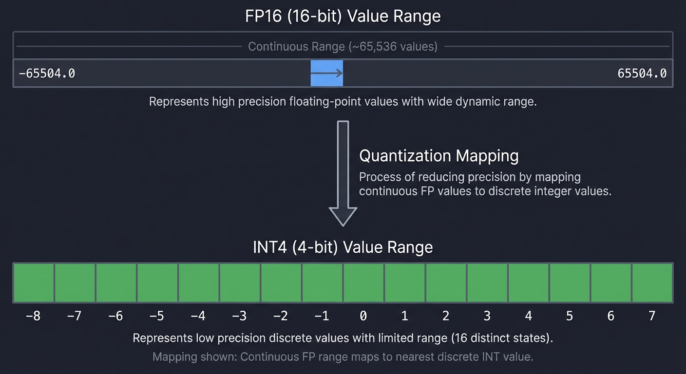
Quantization is the process of mapping high-precision values (FP32/FP16) to a smaller set of discrete levels (INT8/INT4). It’s essentially lossy compression for neural network weights.
FP16 (16-bit) Value Range: ~65,536 values
[ -65504.0 ... 65504.0 ]
       |
       v (Quantization Mapping)
       |
INT4 (4-bit) Value Range: 16 values
[ -8, -7, -6, -5, -4, -3, -2, -1, 0, 1, 2, 3, 4, 5, 6, 7 ]
Key Techniques:
- GPTQ (Post-Training Quantization): Quantizes weights layer-by-layer and compensates for the error by adjusting remaining weights.
- AWQ (Activation-aware Weight Quantization): Identifies the 1% of “salient” weights that are most important for accuracy and protects them from heavy quantization.
- GGUF: A file format optimized for CPU/GPU hybrid inference (llama.cpp), allowing parts of the model to live in system RAM.
2. KV Cache Management: Solving the Memory Eater
In Transformer models, the “Key” and “Value” vectors for every token must be stored to calculate attention for the next token. As the conversation gets longer, the memory needed for these vectors explodes.
The Bottleneck: Traditional LLM inference is Memory-Bound. We spend more time moving data from VRAM to the processor than actually performing the math.
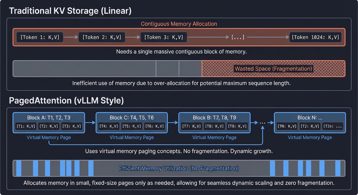
Traditional KV Storage (Linear)
[Token 1: K,V][Token 2: K,V][Token 3: K,V]...[Token 1024: K,V]
^ Needs a single massive contiguous block of memory.

PagedAttention (vLLM Style)
[Block A: T1, T2, T3] -> [Block C: T4, T5, T6] -> [Block B: T7, T8, T9]
^ Uses virtual memory paging concepts. No fragmentation. Dynamic growth.
3. Speculative Decoding: The “Guess and Check” Loop
LLM inference is slow because it’s autoregressive: you must finish Token N before you can even start Token N+1. Speculative decoding breaks this sequence.
The Strategy:
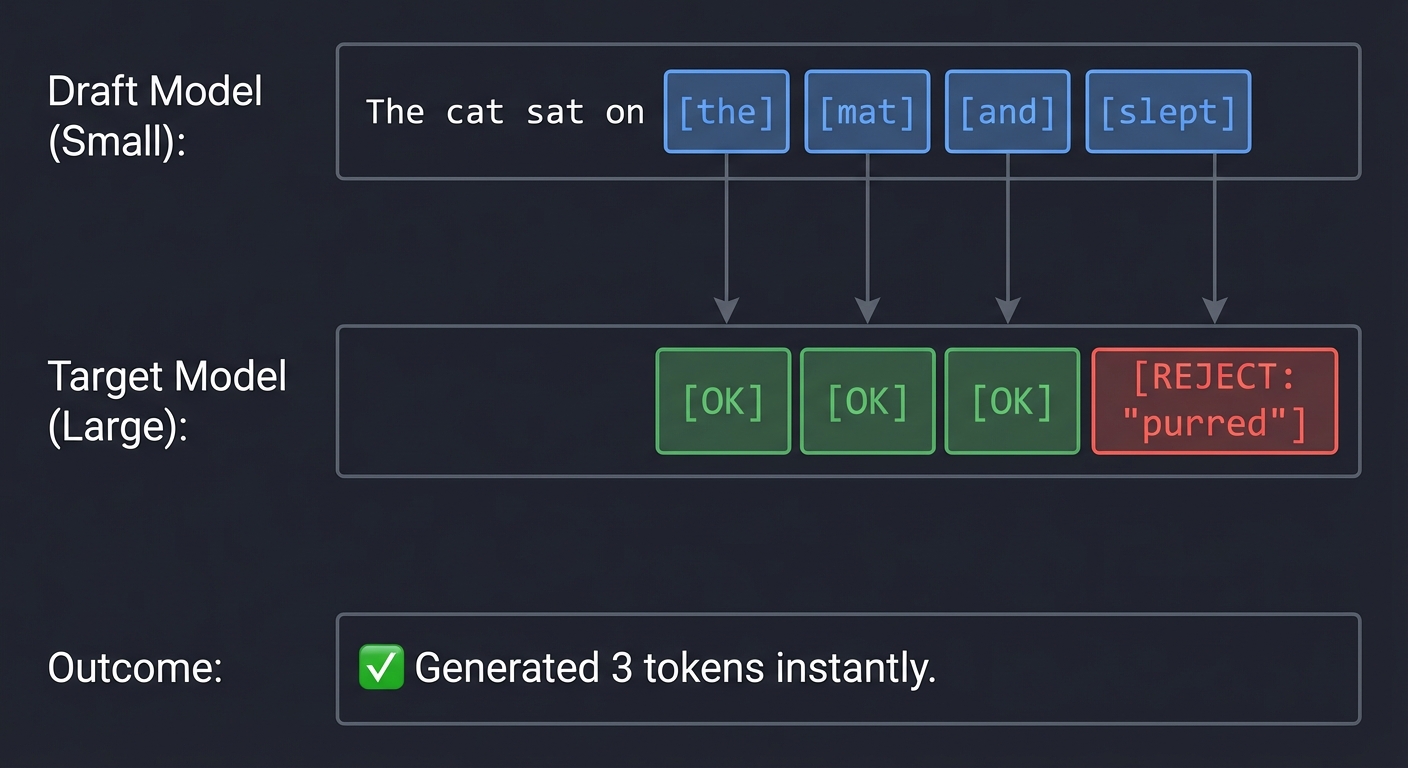
- Use a tiny, “dumb” model (Draft) to guess the next 5 tokens very fast.
- Feed all 5 guesses to the giant, “smart” model (Target) in a single parallel pass.
- The Target model verifies the guesses. If the first 3 were right, we just generated 3 tokens in the time it usually takes to generate 1.
Draft Model (Small):  "The cat sat on [the] [mat] [and] [slept]"
Target Model (Large): [OK]  [OK]  [OK]  [REJECT: "purred"]
Outcome: Generated 3 tokens instantly.
4. Knowledge Distillation: Teacher vs. Student
Distillation is about transferring “dark knowledge” from a massive Teacher (e.g., Llama-3-405B) to a Student (e.g., Llama-3-8B).
Teacher Model (Logits)
[ Cat: 0.92, Dog: 0.07, Car: 0.01 ]
          |
          |  <-- Student tries to match the WHOLE distribution,
          |      not just the "Cat" label.
          v
Student Model
[ Cat: 0.88, Dog: 0.10, Car: 0.02 ]
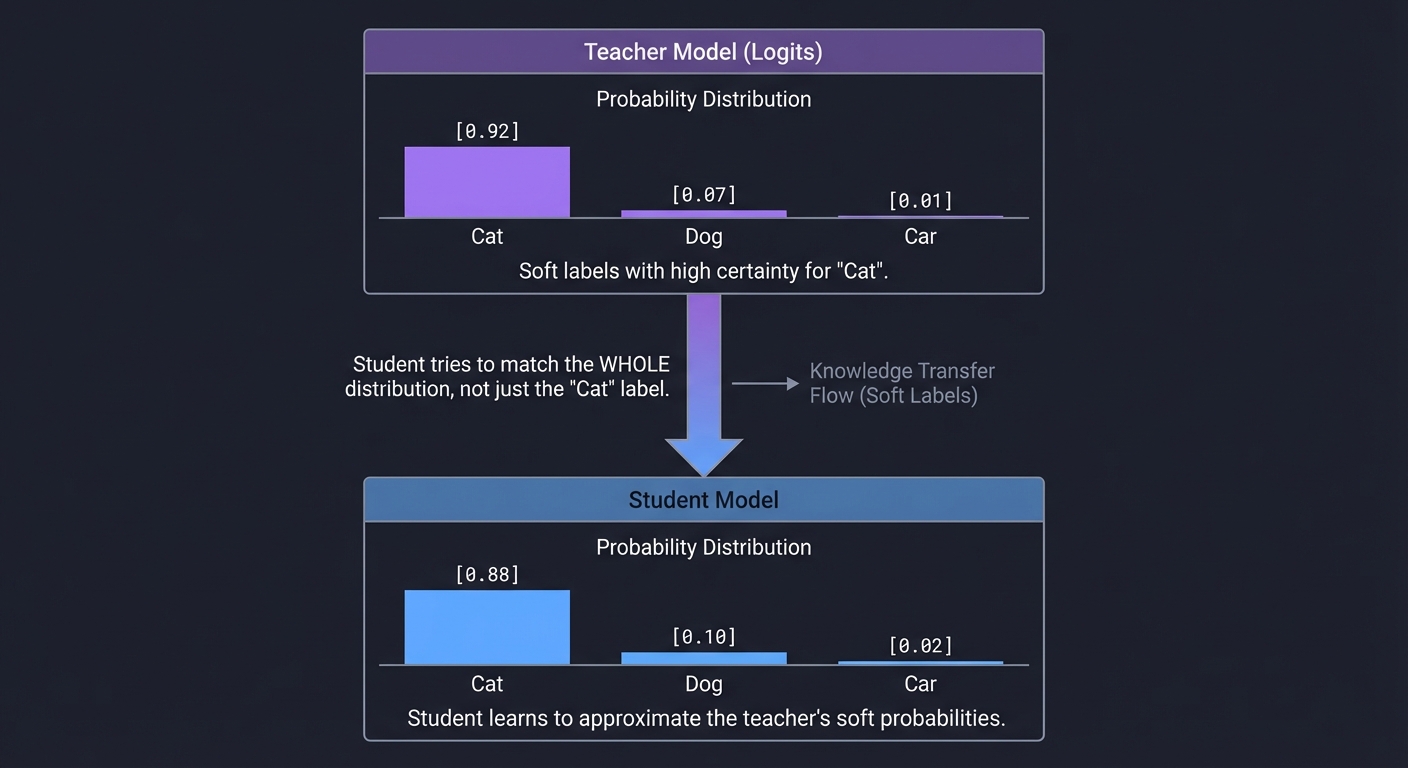 Why it works: The Teacher’s relative probabilities (e.g., “This looks 7% like a dog”) contain rich structural information about the world that a simple “True/False” label misses.
5. Inference Optimization Frameworks
Modern systems don’t just “run” models; they compile them.
- vLLM: Focuses on throughput. Uses PagedAttention to serve hundreds of users simultaneously on one GPU.
- TensorRT-LLM: Focuses on latency. Uses NVIDIA-specific graph optimizations and custom kernels to make a single response as fast as possible.
Concept Summary Table
| Concept Cluster | What You Need to Internalize |
|---|---|
| Quantization | Weights are moved to lower precision (INT4/INT8). GPTQ/AWQ are methods to minimize the resulting accuracy loss. |
| KV Cache | Storing intermediate states to avoid re-computation. PagedAttention is the gold standard for managing this memory. |
| Speculative Decoding | Using a small model to draft and a large model to verify in parallel, bypassing the sequential bottleneck. |
| Distillation | Training a student model to match the teacher’s “soft labels” (probability distributions) rather than just hard truths. |
| Optimization Frameworks | vLLM (Throughput/PagedAttention) vs. TensorRT-LLM (Latency/Graph Fusion). |
Deep Dive Reading by Concept
Quantization & Formats
- GPTQ: “GPTQ: Accurate Post-Training Quantization for Large Language Models” (Frantar et al.)
- AWQ: “AWQ: Activation-aware Weight Quantization for LLM Compression and Acceleration” (Lin et al.)
- GGUF:
llama.cppGitHub README and the GGUF specification.
Memory & Throughput
- PagedAttention: “Efficient Memory Management for Large Language Model Serving with PagedAttention” (vLLM paper)
- FlashAttention: “FlashAttention: Fast and Memory-Efficient Exact Attention with IO-Awareness” (Dao et al.)
Project List
Projects are ordered from foundational understanding to production-grade implementation.
Project 1: The Linear Quantizer (The First Principles)
- File: QUANTIZATION_DISTILLATION_INFERENCE_OPTIMIZATION_MASTERY.md
- Main Programming Language: Python
- Alternative Programming Languages: C++, Rust, Julia
- Coolness Level: Level 4: Hardcore Tech Flex
- Business Potential: 1. The “Resume Gold”
- Difficulty: Level 1: Beginner
- Knowledge Area: Numerical Representation / Linear Algebra
- Software or Tool: NumPy / PyTorch
- Main Book: “Computer Systems: A Programmer’s Perspective” by Bryant & O’Hallaron (Ch. 2: Data Representation)
What you’ll build: A tool that takes a matrix of FP32 weights and manually converts them to INT8 and INT4 using Symmetric and Asymmetric quantization, calculating the scaling factors (S) and zero points (Z) from scratch.
Why it teaches optimization: You’ll discover that quantization isn’t just “rounding.” It’s a mathematical mapping. You’ll see the “quantization error” (the noise added by the process) and how it varies based on the distribution of your weights.
Core challenges you’ll face:
- Calculating the dynamic range → maps to understanding Outliers in neural network weights
- Handling Zero-Point alignment → maps to Asymmetric vs. Symmetric quantization trade-offs
- Bit-packing (4-bit) → maps to Efficient memory storage of sub-byte data
Key Concepts
- Symmetric vs Asymmetric: “A White Paper on Neural Network Quantization” - Nagel et al.
- Scaling Factors: “Quantization and Training of Neural Networks” - Jacob et al. (Google)
Difficulty: Beginner Time estimate: Weekend Prerequisites: Basic Python and NumPy.
Real World Outcome
You will have a Python script that takes any PyTorch tensor and “compresses” it. You’ll see exactly how much memory is saved and how the values shift.
Example Output:
$ python linear_quantizer.py --bits 4 --mode symmetric
[Original] Mean: 0.0012, Std: 0.045, Range: [-1.2, 1.2]
[Quantizing to 4-bit...]
Scale Factor (S): 0.15
Mapping: 1.2 -> 8 (max), -1.2 -> -8 (min)

[Dequantized Stats]
MSE Error: 0.00042
[Memory Saved]: 75.0%

# You will see the histogram of weights becoming "steppy" and discrete!
The Core Question You’re Answering
“What IS a weight? If I change its value by 1%, does the model’s brain break?”
Before you write any code, sit with this. We usually treat weights as precise physical constants. In reality, they are just signals. This project answers how much “noise” we can inject into those signals before the signal becomes garbage.
Concepts You Must Understand First
Stop and research these before coding:
- Floating Point Representation
- How does a computer store 3.1415?
- What is the difference between Mantissa and Exponent?
- Book Reference: “Computer Systems” Ch. 2.4 - Bryant & O’Hallaron
- Linear Mapping
- How do you map the range [-2, 5] to the range [0, 255]?
- What is an affine transformation?
- Book Reference: “Linear Algebra and Its Applications” Ch. 1 - Gilbert Strang
Questions to Guide Your Design
Before implementing, think through these:
- The Dynamic Range
- If 99% of your weights are between -1 and 1, but one weight is 100, where should you set your range?
- What happens if you “clip” the outlier?
- Bit Packing
- A byte is 8 bits. How do you store two 4-bit numbers in a single byte array?
- How do you retrieve the “high nibble” and “low nibble”?
Thinking Exercise
The Rounding Error
Imagine your weights are: [0.1, 0.4, 0.6, 0.9].
You are quantizing to a 1-bit scale (0 or 1).
Questions while tracing:
- If you use a simple threshold of 0.5, what happens to 0.4 and 0.6?
- If these are neurons in a network, how much did the “signal” change for each?
- If you add up the total error for the layer, is it centered around zero?
The Interview Questions They’ll Ask
Prepare to answer these:
- “What is the difference between Symmetric and Asymmetric quantization?”
- “Why do outliers make quantization difficult?”
- “Explain the formula: W = S(Q - Z).”
- “What is a ‘Zero Point’ and why do we need it for activations but maybe not for weights?”
- “How does INT8 quantization speed up inference on hardware that lacks a floating-point unit?”
Hints in Layers
Hint 1: The Formula The fundamental mapping is Q = clamp(round(W/S) + Z). Your job is to find S (Scale) and Z (Zero-point).
Hint 2: Calculating Scale For Symmetric quantization, Z=0 and S = max(|min|, |max|) / (2^{bits-1} - 1).
Hint 3: Bit Packing in Python
To pack two 4-bit values a and b into one 8-bit byte: packed = (a << 4) | (b & 0x0F).
Hint 4: NumPy Vectorization Don’t use loops! Use np.round, np.clip, and np.max to process the whole matrix at once.
Books That Will Help
| Topic | Book | Chapter |
|---|---|---|
| Data Representation | “Computer Systems: A Programmer’s Perspective” | Ch. 2 |
| Quantization Math | “A White Paper on Neural Network Quantization” | Sections 2-3 |
Project 2: GPTQ Calibration Workbench
- File: QUANTIZATION_DISTILLATION_INFERENCE_OPTIMIZATION_MASTERY.md
- Main Programming Language: Python
- Alternative Programming Languages: C++ (with LibTorch)
- Coolness Level: Level 3: Genuinely Clever
- Business Potential: 4. The “Open Core” Infrastructure
- Difficulty: Level 3: Advanced
- Knowledge Area: Optimization / Hessian Matrices
- Software or Tool: PyTorch / AutoGPTQ (internals)
- Main Book: “Algorithms for Optimization” by Mykel J. Kochenderfer
What you’ll build: A mini-GPTQ implementer that quantizes a single Transformer layer. You will use a small “calibration set” (e.g., 128 tokens of text) to observe the activations and use the Inverse Hessian matrix to decide how to adjust weights to compensate for quantization noise.
Why it teaches optimization: You’ll move from “static” quantization (Project 1) to “data-aware” quantization. You’ll learn why we need sample data (calibration) to quantize models without making them incoherent.
Core challenges you’ll face:
- Layer-wise error minimization → maps to Understanding that errors propagate through the network
- Approximating the Hessian → maps to The math of “which weights matter most”
- Sequential weight updates → maps to The OBQ (Optimal Brain Quantizer) algorithm
Key Concepts
- Optimal Brain Surgeon: “Optimal Brain Surgeon and General Network Pruning” - Hassibi et al.
- GPTQ Math: “GPTQ: Accurate Post-Training Quantization” - Frantar et al.
Difficulty: Advanced Time estimate: 1-2 weeks Prerequisites: Project 1, solid Linear Algebra (Matrix inverses, derivatives).
Real World Outcome
You will see how a layer’s output changes when weights are adjusted via GPTQ logic versus simple rounding.
Example Output:
$ python gptq_layer.py --layer attn.q_proj --calibrate wiki.txt
[Step 1] Computing Hessian for layer inputs...
[Step 2] Quantizing block 1/128...
[Step 3] Adjusting remaining weights...

Output Difference (MSE) vs Original:
Naive Rounding: 0.045
GPTQ Compensation: 0.0012
# Huge improvement in fidelity!
The Core Question You’re Answering
“If I break one weight, can I ‘fix’ the damage by slightly changing the weights next to it?”
This is the central insight of GPTQ. Neural networks are robust. If you quantize one weight and it’s slightly too small, you can compensate by making its neighbor slightly larger.
Concepts You Must Understand First
Stop and research these before coding:
- Second-Order Optimization
- What is a Hessian matrix?
- Why does the Hessian tell us about the “curviness” of the loss surface?
- Book Reference: “Algorithms for Optimization” Ch. 4 - Kochenderfer
- Calibration Data
- Why do we need data to quantize?
- What is the “distribution of activations”?
Questions to Guide Your Design
Before implementing, think through these:
- Computational Cost
- Calculating the full Inverse Hessian is $O(N^3)$. How does GPTQ approximate this to make it feasible for billions of weights?
- Block-wise Processing
- Should you quantize the whole layer at once or break it into blocks? Why?
Thinking Exercise
The Ripple Effect
Imagine a row of 3 weights: [1.0, 1.0, 1.0]. You quantize the first weight to 1.2.
Questions while tracing:
- To keep the total sum of the row at
3.0, what should the other two weights become? - How does this logic scale when you have a 4096-dimensional vector?
The Interview Questions They’ll Ask
Prepare to answer these:
- “Why is GPTQ called ‘Post-Training’?”
- “What is the role of calibration data in GPTQ?”
- “Explain the OBQ (Optimal Brain Quantizer) algorithm at a high level.”
- “How does GPTQ handle the numerical stability of the Inverse Hessian?”
- “What is the computational complexity of GPTQ per layer?”
Hints in Layers
Hint 1: The Greedy Approach Start by quantizing one weight at a time and calculating the error.
Hint 2: The Hessian Shortcut GPTQ uses the fact that we are minimizing a quadratic error. Look up the “Sherman-Morrison formula” for efficient inverse updates.
Hint 3: Activation Magnitudes Recall that weights interact with activations. If an input activation is always 0, its corresponding weight doesn’t matter! This is why we calibrate.
Books That Will Help
| Topic | Book | Chapter |
|---|---|---|
| Optimization | “Algorithms for Optimization” | Ch. 4, 12 |
| GPTQ Logic | “GPTQ: Accurate Post-Training Quantization” (Paper) | Section 3 |
Real World Outcome
You will have a tool that can peek inside any Llama-3 or Mistral model file and tell you exactly how it was built.
Example Output:
$ ./gguf-peek Llama-3-8B-Q4_K_M.gguf
--- GGUF Header ---
Magic: GGUF
Version: 3
Tensors: 291
Metadata KV: 18

--- Metadata ---
general.name: Llama-3-8B
llama.context_length: 8192
tokenizer.ggml.model: gpt2

--- Tensors ---
token_embd.weight: [128256, 4096] (Q4_K)
blk.0.attn_q.weight: [4096, 4096] (Q4_K)
...
The Core Question You’re Answering
“How do I load a 50GB file into memory in less than 1 second?”
GGUF answers this through mmap. This project forces you to see how binary alignment makes this possible.
Concepts You Must Understand First
Stop and research these before coding:
- Endianness
- What is the difference between Big-Endian and Little-Endian?
- Why do modern CPUs prefer Little-Endian?
- Memory Mapping (mmap)
- How does a program access a file as if it were an array in memory?
- What is a “page fault”?
Questions to Guide Your Design
Before implementing, think through these:
- Version Compatibility
- How does GGUF handle adding new metadata fields without breaking older parsers?
- Padding
- Why are tensors aligned to 32 or 64-byte boundaries? (Hint: SIMD instructions).
Thinking Exercise
The Byte Stream
Open a GGUF file in a hex editor. Look at the first 4 bytes.
Questions while tracing:
- Do you see the letters ‘G’, ‘G’, ‘U’, ‘F’?
- How many bytes follow the header before you reach the first tensor name?
- Can you find the “context_length” string in the metadata section?
The Interview Questions They’ll Ask
Prepare to answer these:
- “What are the advantages of GGUF over the older GGML format?”
- “Why is GGUF preferred for local inference on consumer hardware?”
- “Explain how metadata and tensors are co-located in GGUF.”
- “What does it mean for a file to be ‘mmap-friendly’?”
- “How does GGUF handle model architectures beyond Llama?”
Hints in Layers
Hint 1: The Magic Number
Every GGUF file starts with 0x47 0x47 0x55 0x46. Read 4 bytes and check this first.
Hint 2: Structural Offsets The header tells you how many KV pairs exist. You must iterate through them one by one to find where the Tensor section begins.
Hint 3: String Parsing
GGUF strings are length-prefixed. Read an 8-byte uint64_t first, then read that many bytes of text.
Project 4: KV Cache “OOM” Simulator
- File: QUANTIZATION_DISTILLATION_INFERENCE_OPTIMIZATION_MASTERY.md
- Main Programming Language: Python (with Visualization)
- Alternative Programming Languages: JavaScript (React/D3)
- Coolness Level: Level 5: Pure Magic
- Business Potential: 5. The “Industry Disruptor”
- Difficulty: Level 3: Advanced
- Knowledge Area: Memory Management / Distributed Systems
- Software or Tool: PyTorch / Matplotlib
- Main Book: “Operating Systems: Three Easy Pieces” (Ch. 18-20: Paging)
What you’ll build: A visual simulator that tracks the memory consumption of an LLM as it processes a batch of requests. You will implement two allocators:
- The Naive Allocator: Allocates contiguous blocks (leads to Out-of-Memory quickly due to fragmentation).
- The PagedAttention Allocator: Splits KV Cache into 16-token “pages” and maps them dynamically.
Why it teaches optimization: This is the core innovation behind vLLM. You’ll see exactly why “standard” memory allocation fails for LLMs and how OS-level paging concepts saved the inference industry.
Core challenges you’ll face:
- Calculating KV tensor size per token → maps to Attention Head math (Batch x Heads x Dim)
- External vs Internal Fragmentation → maps to Efficient VRAM utilization
- Mapping Logical vs Physical pages → maps to The PagedAttention algorithm
Difficulty: Advanced Time estimate: 1-2 weeks Prerequisites: Understanding of the Transformer Attention mechanism (Q, K, V).
Real World Outcome
You’ll see a graph showing memory usage over time. The Naive allocator will “crash” (OOM) at 5 requests, while the PagedAttention allocator will handle 25 requests on the same memory budget.
Example Output:
$ python vllm_sim.py --total-vram 16GB --requests 50
[Naive Allocator]
Request 1: Allocated 2GB (Indices 0-2000)
Request 2: Allocated 4GB (Indices 2000-6000)
...
Request 5: ERROR - Out of Memory (Need 3GB, Largest Hole 1.5GB)
Total Tokens Served: 4,500

[PagedAttention Allocator]
Request 1: Logical -> [Phys Block 1, 5, 12]
Request 2: Logical -> [Phys Block 2, 8, 3]
...
Request 25: Memory Full (Gracefully waiting for release)
Total Tokens Served: 18,200
The Core Question You’re Answering
“Why is GPU memory ‘full’ when I still have gigabytes of space left?”
The answer is Fragmentation. This project teaches you that managing memory for dynamic-length sequences (LLMs) is an Operating Systems problem, not just a Deep Learning problem.
Concepts You Must Understand First
Stop and research these before coding:
- Virtual Memory & Paging
- What is a Page Table?
- What is the difference between a physical address and a logical address?
- Book Reference: “Operating Systems: Three Easy Pieces” Ch. 18
- KV Cache Calculation
- How many bytes does one token take in Llama-3-8B? (Hint: 2 layers * heads * dim * precision).
Questions to Guide Your Design
Before implementing, think through these:
- Block Size
- If a block is 1 token, the page table is huge. If a block is 1024 tokens, we waste memory. Why is 16 the industry standard?
- Sharing
- If two requests share the same prefix (e.g., the same system prompt), can they share the same physical blocks? How?
Thinking Exercise
The Tetris Problem
Imagine a memory bar of 10 slots.
- Request A needs 3 slots.
- Request B needs 3 slots.
- Request C needs 3 slots.
- Total used: 9. Slot 10 is free.
- Request A finishes. Slots 1, 2, 3 are free.
- Request D comes in and needs 4 slots.
Questions while tracing:
- In a “naive” contiguous system, can Request D start?
- In a “paged” system, can Request D start?
The Interview Questions They’ll Ask
Prepare to answer these:
- “What is PagedAttention and why is it needed?”
- “How does vLLM handle external fragmentation?”
- “Explain the mapping between logical token indices and physical GPU blocks.”
- “What are the benefits of prefix caching in a paged system?”
- “How do you calculate the maximum batch size for a model given its KV cache size?”
Hints in Layers
Hint 1: The Math A single token’s KV cache size = 2 * Layers * Heads * HeadDim * PrecisionBytes.
Hint 2: The Block Manager Create a FreeList of block IDs. When a request starts, pop IDs from the list.
Hint 3: Logical Mapping
Use a dictionary where (request_id, token_index // block_size) maps to a physical_block_id.
Books That Will Help
| Topic | Book | Chapter |
|---|---|---|
| Paging | “Operating Systems: Three Easy Pieces” | Ch. 18-20 |
| vLLM Architecture | “PagedAttention” Paper | Sections 2-4 |
Project 5: Speculative Decoding Simulator
- File: QUANTIZATION_DISTILLATION_INFERENCE_OPTIMIZATION_MASTERY.md
- Main Programming Language: Python
- Alternative Programming Languages: C++
- Coolness Level: Level 5: Pure Magic
- Business Potential: 5. The “Industry Disruptor”
- Difficulty: Level 3: Advanced
- Knowledge Area: Algorithm Design / Probability
- Software or Tool: PyTorch / Transformers
- Main Book: “Fast Inference from Transformers via Speculative Decoding” (Original Paper)
What you’ll build: A system where a tiny “Draft” model (e.g., Llama-160M) predicts tokens for a “Target” model (e.g., Llama-7B). You will implement the rejection sampling logic and measure the “Speedup Factor” and “Acceptance Rate.”
Why it teaches optimization: You’ll understand the statistical nature of LLMs. You’ll learn that we can “borrow” compute from the future if we can guess correctly, and that verification is much cheaper than generation.
Core challenges you’ll face:
- Rejection Sampling implementation → maps to Ensuring the output is statistically identical to the Target model
- Synchronizing KV Caches → maps to Managing state between two different models
- Measuring latency vs. throughput → maps to Understanding when Speculative Decoding actually helps
Real World Outcome
You will see a live “speedometer” showing how many tokens are accepted per draft run.
Example Output:
$ python speculative_decoding.py --draft tiny-llama --target llama-7b
Prompt: "Once upon a time in a"
Draft Guess: [distant] [galaxy] [far] [away]
Target Check: [OK]      [OK]     [OK]  [REJECT: "very"]

Batch Speedup: 3.2x (3 tokens accepted in 1 target pass)
Total Speedup: 2.1x over 100 tokens.
The Core Question You’re Answering
“Can a ‘dumb’ model help a ‘smart’ model think faster?”
Yes, because most English tokens are predictable. “The cat sat on the…” is almost certainly followed by “mat.” The small model can guess the obvious parts, leaving the big model to only think about the hard parts.
Concepts You Must Understand First
Stop and research these before coding:
- Rejection Sampling
- How do you sample from Distribution A while ensuring the result matches Distribution B?
- Autoregressive Bottleneck
- Why can’t we just generate 10 tokens at once in a normal Transformer?
Questions to Guide Your Design
Before implementing, think through these:
- Draft Length (K)
- If you guess 10 tokens and only 1 is right, you wasted time. If you guess 2 and both are right, you could have guessed more. How do you find the optimal K?
- Model Alignment
- If the Draft model uses a different tokenizer than the Target model, can speculative decoding still work? (Hint: It’s much harder).
Thinking Exercise
The Assistant
Imagine you are a fast typist (Draft) and your boss is a slow but brilliant editor (Target).
- You type 5 words.
- Your boss looks at all 5 at once.
- He deletes the words he doesn’t like and continues from there.
Questions while tracing:
- If your boss deletes the 2nd word, what happens to words 3, 4, and 5?
- How much time did you save if your boss liked all 5 words?
The Interview Questions They’ll Ask
Prepare to answer these:
- “What is Speculative Decoding?”
- “Why is it considered a ‘lossless’ optimization?”
- “Explain the rejection sampling condition in speculative decoding.”
- “When does speculative decoding become SLOWER than standard decoding?”
- “What is the relationship between the Draft model’s accuracy and the total speedup?”
Hints in Layers
Hint 1: The Probability Ratio
You accept a token x if rand() < P_target(x) / P_draft(x).
Hint 2: Parallel Verification The Target model takes the original sequence + all K drafted tokens as a single batch.
Hint 3: KV Cache Rewinding When the Target model rejects a token, you must “rewind” the KV cache to that position before the next draft run.
Books That Will Help
| Topic | Book | Chapter |
|---|---|---|
| Speculative Decoding | “Fast Inference” Paper | Sections 3-4 |
| Probability | “Grokking Deep Learning” | Ch. 4 |
Project 6: Knowledge Distillation Trainer (MLP Version)
- File: QUANTIZATION_DISTILLATION_INFERENCE_OPTIMIZATION_MASTERY.md
- Main Programming Language: Python
- Alternative Programming Languages: N/A
- Coolness Level: Level 3: Genuinely Clever
- Business Potential: 1. The “Resume Gold”
- Difficulty: Level 2: Intermediate
- Knowledge Area: Model Training / Optimization
- Software or Tool: PyTorch / Keras
- Main Book: “Deep Learning” by Ian Goodfellow (Ch. 14: Autoencoders/Representation Learning)
What you’ll build: You’ll train a “Teacher” MLP on a complex dataset (like MNIST or CIFAR-10). Then, you’ll train a 10x smaller “Student” MLP using two losses: the standard ground-truth loss and the KL-Divergence loss from the Teacher’s “soft labels” (at high temperature).
Why it teaches optimization: You’ll see that “Dark Knowledge” is real. The Student trained with Distillation will significantly outperform a Student trained only on raw labels.
Core challenges you’ll face:
- Tuning the Temperature (T) → maps to Smoothing the probability distribution
- Balancing alpha (teacher weight) → maps to Learning from truth vs. learning from intuition
- Observing the “Gap” → maps to Understanding the limits of model compression
Real World Outcome
A comparison chart showing accuracy of:
- Large Teacher
- Small Student (Baseline)
- Small Student (Distilled)
Example Output:
$ python distill.py --teacher-size 2048 --student-size 128
Teacher Accuracy: 98.2%
Student Baseline Accuracy: 89.1%
Student Distilled Accuracy: 94.5%

# The distilled student is nearly as smart as the teacher despite being 16x smaller!
The Core Question You’re Answering
“If the answer is ‘Cat’, why does it matter if the model also thinks it’s 10% ‘Dog’?”
Because that 10% “Dog” contains the information that cats and dogs share features (fur, ears, tails). This “Dark Knowledge” helps the small student model learn the underlying structure of the world much faster than just looking at hard labels.
Concepts You Must Understand First
Stop and research these before coding:
- Kullback-Leibler (KL) Divergence
- How do you measure the distance between two probability distributions?
- Softmax Temperature
- Why does dividing logits by T > 1 make the distribution flatter?
Questions to Guide Your Design
Before implementing, think through these:
- The Temperature Trade-off
- If T is too high, the distribution is just noise. If T is 1, it’s just the max label. Where is the “Knowledge”?
- Model Mismatch
- Can a Teacher using ReLU train a Student using Sigmoid? Why or why not?
Thinking Exercise
The Teacher’s Grades
Imagine a test with 4 choices.
- The correct answer is A.
- The Teacher model says: A (80%), B (18%), C (1%), D (1%).
- Another Teacher says: A (80%), B (7%), C (6%), D (7%).
Questions while tracing:
- Which Teacher provides more “information” about why the answer is A?
- How does the student model use the 18% in choice B to learn?
The Interview Questions They’ll Ask
Prepare to answer these:
- “What is ‘Dark Knowledge’ in model distillation?”
- “How does the temperature parameter T affect the distillation process?”
- “Explain the components of the distillation loss function.”
- “Can you distill a model into a different architecture (e.g., ResNet to ViT)?”
- “What are the limitations of distillation? Why can’t we distill GPT-4 into a 1-million parameter model?”
Hints in Layers
Hint 1: The High-Temp Softmax
Apply softmax(logits / T) to both the teacher and the student outputs before calculating KL loss.
Hint 2: The Multiplier Hinton’s paper suggests multiplying the distillation loss by T^2 to keep the gradients at the same scale as the student loss.
Hint 3: Freezing the Teacher
Don’t forget to set teacher.eval() and requires_grad = False for the teacher model. You are only training the student!
Books That Will Help
| Topic | Book | Chapter |
|---|---|---|
| Distillation | “Distilling Knowledge” Paper | Sections 2-3 |
| Entropy | “Information Theory” | Ch. 2 |
Project 7: Benchmarking Quantization Loss (The PPL Tool)
- File: QUANTIZATION_DISTILLATION_INFERENCE_OPTIMIZATION_MASTERY.md
- Main Programming Language: Python
- Alternative Programming Languages: Shell
- Coolness Level: Level 2: Practical but Forgettable
- Business Potential: 3. The “Service & Support” Model
- Difficulty: Level 2: Intermediate
- Knowledge Area: Performance Analysis / NLP Metrics
- Software or Tool: LM Evaluation Harness / PyTorch
- Main Book: “Speech and Language Processing” by Jurafsky & Martin (Ch. 3: N-gram Language Models)
What you’ll build: A benchmarking suite that calculates the Perplexity (PPL) of a model on the WikiText-2 dataset. You will compare a base model (FP16) against INT8, GPTQ 4-bit, and AWQ 4-bit versions.
Why it teaches optimization: You’ll learn that “it works” isn’t enough. You need objective metrics to see if quantization “broke” the model’s brain. You’ll discover that some tasks are more “quantization-sensitive” than others.
Core challenges you’ll face:
- Calculating Perplexity correctly → maps to Understanding the Cross-Entropy of the language model
- Handling different tokenizers → maps to Ensuring benchmarks are fair across formats
- Visualizing the “Degradation Curve” → maps to Deciding when 4-bit is “good enough”
Real World Outcome
You’ll produce a report that helps you decide which quantization method to use for a production app.
Example Output:
$ python benchmark_ppl.py --model llama-3-8b --quants fp16,gptq-4bit,awq-4bit
| Format    | WikiText-2 PPL | Accuracy (MMLU) | VRAM Used |
|-----------|----------------|-----------------|-----------|
| FP16      | 5.42           | 66.5%           | 16.0 GB   |
| GPTQ 4-bit| 5.61           | 65.8%           | 5.2 GB    |
| AWQ 4-bit | 5.58           | 66.1%           | 5.2 GB    |

# You've just proved that 4-bit saves 67% memory with only ~1% accuracy drop!
The Core Question You’re Answering
“How much ‘stupider’ did my model get after I compressed it?”
Perplexity is the standard measure of how “confused” a model is by real text. This project teaches you how to quantify that confusion.
Concepts You Must Understand First
Stop and research these before coding:
- Information Entropy
- What does it mean for a probability distribution to have high entropy?
- Perplexity (PPL)
- Why is PPL defined as exp(AverageCrossEntropy)?
Questions to Guide Your Design
Before implementing, think through these:
- Context Length
- Does PPL change if you measure it with a context of 512 tokens versus 2048?
- Sensitivity
- Why might a model’s PPL remain good while its ability to write Python code is destroyed? (Hint: Code is less redundant than natural language).
Thinking Exercise
The Surprise Factor
Imagine a model is predicting the next letter in “The cat sat on the m_”.
- Prediction 1: ‘a’ (99%)
- Prediction 2: ‘o’ (99%)
Questions while tracing:
- If the true letter is ‘a’, which prediction has lower cross-entropy?
- If the true letter is ‘u’, how does the Perplexity jump?
The Interview Questions They’ll Ask
Prepare to answer these:
- “What is Perplexity and why is it used for LLM evaluation?”
- “How do quantization artifacts manifest in model performance?”
- “Which quantization method (GPTQ vs AWQ) typically yields lower PPL?”
- “Why is PPL alone not sufficient for evaluating a model’s capabilities?”
- “Explain how bit-width (8-bit vs 4-bit) affects the PPL curve.”
Hints in Layers
Hint 1: The Cross-Entropy Loss
In PyTorch, nn.CrossEntropyLoss() is your friend. Just remember it expects logits and true token IDs.
Hint 2: Sliding Window For WikiText-2, don’t just take the first 2048 tokens. Use a sliding window to measure PPL across the whole text.
Hint 3: Precision
Even when measuring a 4-bit model, calculate the loss in FP32 to avoid numerical overflow in the exp() function.
Books That Will Help
| Topic | Book | Chapter |
|---|---|---|
| Perplexity | “Speech and Language Processing” | Ch. 3 |
| Evaluation | “NLP with Transformers” | Ch. 8 |
Project 8: vLLM-lite (PagedAttention Implementation)
- File: QUANTIZATION_DISTILLATION_INFERENCE_OPTIMIZATION_MASTERY.md
- Main Programming Language: Python
- Alternative Programming Languages: C++
- Coolness Level: Level 5: Pure Magic
- Business Potential: 5. The “Industry Disruptor”
- Difficulty: Level 4: Expert
- Knowledge Area: Systems Architecture / Memory Management
- Software or Tool: PyTorch / Custom Allocators
- Main Book: “Efficient Memory Management for Large Language Model Serving with PagedAttention” (vLLM Paper)
What you’ll build: A mock inference server that simulates the PagedAttention memory layout. You’ll implement a BlockManager that manages a “Pool” of physical blocks and a “Logical” mapping for each request.
Why it teaches optimization: This is the most important technical concept in modern LLM serving. You’ll understand how we can serve 10 concurrent requests without needing 10x the memory.
Core challenges you’ll face:
- Block mapping logic → maps to The virtual-to-physical address translation
- Copy-on-Write for parallel sampling → maps to Efficient beam search implementation
- Handling variable sequence lengths → maps to The core problem of LLM memory fragmentation
Real World Outcome
A simulation where you can see physical memory blocks being assigned and reclaimed in real-time.
Example Output:
$ python paged_attn.py --sim-requests 3
Request 1: logical[0:16] -> physical[42]
Request 1: logical[16:32] -> physical[7]
Request 2: logical[0:16] -> physical[42] (SHARED PREFIX!)

Memory Map: [B1:R1, B2:Free, B3:R2, ..., B42:R1+R2]
The Core Question You’re Answering
“How do I manage memory when I don’t know how long the output will be?”
PagedAttention solves this by treating VRAM like an OS treats RAM—using pages instead of contiguous buffers.
Concepts You Must Understand First
Stop and research these before coding:
- Physical vs Logical Memory
- How does an OS mask the fact that memory is fragmented?
- Reference Counting
- How do you know when it’s safe to delete a shared memory block?
Questions to Guide Your Design
Before implementing, think through these:
- Eviction Policy
- If memory is full and a new token is generated, which request do you pause?
- Block Sharing
- How do you detect that two different requests are using the same “System Prompt” to enable sharing?
Thinking Exercise
The Library
Imagine a library with 1000 shelves.
- A student (Request) asks for space to write a book.
- You don’t know if the book will be 10 pages or 500.
Questions while tracing:
- If you give every student a whole aisle, how many students can you fit?
- If you give every student 1 shelf at a time, how do they find their “next” shelf when they move to another aisle?
The Interview Questions They’ll Ask
Prepare to answer these:
- “What is PagedAttention?”
- “Why does vLLM outperform Hugging Face TGI?”
- “Explain how prefix caching works in a paged system.”
- “What is the ‘waste’ (internal fragmentation) in PagedAttention?”
- “How does the scheduler decide when to ‘preempt’ a request?”
Hints in Layers
Hint 1: The Logical Table
Maintain a mapping: Map<RequestId, List
Hint 2: Shared Blocks Use a Hash(PrefixTokens) to identify if a block can be shared. Use a reference count to manage its lifetime.
Hint 3: Sequence Growth Every time a request generates block_size tokens, it must ask the BlockManager for a new physical block ID.
Books That Will Help
| Topic | Book | Chapter |
|---|---|---|
| PagedAttention | vLLM Paper | Full Paper |
| Virtual Memory | “CS:APP” | Ch. 9 |
Project 10: The Local “Llama-in-a-Box” (Production Grade)
- File: QUANTIZATION_DISTILLATION_INFERENCE_OPTIMIZATION_MASTERY.md
- Main Programming Language: Python / Docker / Bash
- Alternative Programming Languages: Go
- Coolness Level: Level 2: Practical but Forgettable
- Business Potential: 4. The “Open Core” Infrastructure
- Difficulty: Level 2: Intermediate
- Knowledge Area: MLOps / Systems Deployment
- Software or Tool: vLLM / Docker / Nginx
- Main Book: “Designing Data-Intensive Applications” by Martin Kleppmann
What you’ll build: A production-ready inference API using vLLM in a Docker container. It will support batching, streaming, and health checks. You will set up an Nginx load balancer to distribute requests across multiple instances.
Why it teaches optimization: This is the “real world” application of everything else. You’ll see how PagedAttention (vLLM) and Quantization (GPTQ) allow you to serve multiple users on a single consumer GPU.
Core challenges you’ll face:
- Configuring vLLM for high throughput → maps to Optimizing the engine for the hardware
- Implementing “Continuous Batching” → maps to Modern LLM scheduling
- Handling GPU memory limits in Docker → maps to Containerized AI infrastructure
Real World Outcome
You’ll have a URL that anyone in your local network can use to get LLM answers at 100+ tokens per second.
Example Output:
$ curl -X POST http://localhost/v1/completions -d '{"model": "llama-3-8b", "prompt": "Once upon a time"}'
{
  "id": "cmpl-123",
  "choices": [{"text": " in a land far away..."}],
  "usage": {"total_tokens": 25}
}

# You are now running your own OpenAI-compatible API!
The Core Question You’re Answering
“How do I take a model from a Python script and make it a reliable service?”
This project teaches you the gap between “research code” and “production engineering.”
Concepts You Must Understand First
Stop and research these before coding:
- REST APIs vs. WebSockets
- Why is streaming (Server-Sent Events) preferred for LLMs?
- Load Balancing
- How do you share traffic between two GPUs?
Questions to Guide Your Design
Before implementing, think through these:
- Queueing
- If 100 people ask a question at once, how does the system decide who goes first?
- Monitoring
- How do you measure “Tokens per Second” per user?
Thinking Exercise
The Restaurant
Imagine an LLM is a chef.
- Traditional: The chef makes one meal, serves it, then starts the next.
- Continuous Batching: The chef has 5 pans. While one steak is searing, he chops onions for the next meal.
Questions while tracing:
- If meal A takes 5 minutes and meal B takes 2 minutes, should the chef wait for A to finish before starting B?
The Interview Questions They’ll Ask
Prepare to answer these:
- “What is Continuous Batching?”
- “How do you handle rate limiting for an LLM API?”
- “Explain the benefits of running vLLM inside Docker.”
- “How do you monitor VRAM usage in production?”
- “What is the difference between latency and throughput in LLM serving?”
Hints in Layers
Hint 1: vLLM Docker Image Use the official vLLM Docker image as your base. Don’t build from scratch unless you have to.
Hint 2: OpenAI Compatibility vLLM provides an OpenAI-compatible server out of the box. Focus on configuring it.
Hint 3: Nginx Config
Use proxy_pass to route traffic to the Docker container.
Books That Will Help
| Topic | Book | Chapter |
|---|---|---|
| Systems Design | “Designing Data-Intensive Applications” | Ch. 1, 9 |
| Docker | “Docker Deep Dive” | Ch. 2 |
Project 11: Multi-GPU Quantization Orchestrator
- File: QUANTIZATION_DISTILLATION_INFERENCE_OPTIMIZATION_MASTERY.md
- Main Programming Language: Python
- Alternative Programming Languages: Rust
- Coolness Level: Level 4: Hardcore Tech Flex
- Business Potential: 4. The “Open Core” Infrastructure
- Difficulty: Level 4: Expert
- Knowledge Area: Distributed Computing / Model Parallelism
- Software or Tool: PyTorch / Accelerate / DeepSpeed
- Main Book: “Computer Architecture: A Quantitative Approach” by Hennessy & Patterson
What you’ll build: A tool that takes a massive model (e.g., 70B parameters) and splits it across two GPUs. One GPU runs the first half in 4-bit (to save space), and the second GPU runs the second half in 8-bit (to preserve accuracy for the final layers).
Why it teaches optimization: You’ll master Pipeline Parallelism and the hardware trade-offs of splitting models. You’ll learn that models aren’t monolithic—different parts have different sensitivity to quantization.
Core challenges you’ll face:
- Cross-GPU communication (NCCL) → maps to Data transfer bottlenecks
- Heterogeneous quantization → maps to Managing different data types in one pipeline
- Balancing the pipeline → maps to Ensuring one GPU isn’t waiting for the other
Real World Outcome
You’ll be able to run a model that is physically too large for a single GPU.
Example Output:
$ python distributed_quant.py --model llama-70b --gpus 0,1
GPU 0: Loading Layers 0-40 (INT4) - VRAM: 22GB
GPU 1: Loading Layers 41-80 (INT8) - VRAM: 42GB

[Inference Test]: Successfully generated 50 tokens.
# You just ran a 70B model on consumer hardware!
The Core Question You’re Answering
“How do I make two computers act as one brain?”
This project teaches you how to orchestrate distributed resources for a single task.
Concepts You Must Understand First
Stop and research these before coding:
- Pipeline Parallelism
- How does data flow from GPU A to GPU B?
- NCCL (NVIDIA Collective Communications Library)
- What is an “All-Reduce” operation?
Questions to Guide Your Design
Before implementing, think through these:
- The “Seam”
- What happens at the boundary where the model moves from 4-bit to 8-bit?
- Latency
- Is it faster to have one slow GPU or two fast GPUs communicating?
Thinking Exercise
The Bucket Brigade
Imagine 10 people in a line passing buckets of water.
- Person 1-5 has small buckets (4-bit).
- Person 6-10 has large buckets (8-bit).
Questions while tracing:
- What happens at Person 6? Do they have to wait for two small buckets to fill one large one?
The Interview Questions They’ll Ask
Prepare to answer these:
- “What is Pipeline Parallelism?”
- “How do you handle communication overhead between GPUs?”
- “Explain the trade-offs of heterogeneous quantization.”
- “What is the role of DeepSpeed in LLM optimization?”
- “How do you debug an OOM that only happens on GPU 1 but not GPU 0?”
Hints in Layers
Hint 1: Device Map
Use the device_map parameter in the transformers library to specify which layers go where.
Hint 2: Quantization Config
Create two separate BitsAndBytesConfig objects for the two halves of the model.
Hint 3: Monitoring
Use watch nvidia-smi to see the VRAM usage on both GPUs simultaneously.
Books That Will Help
| Topic | Book | Chapter |
|---|---|---|
| Computer Arch | “Quantitative Approach” | Ch. 4 |
| Distributed PyTorch | PyTorch Documentation | Distributed RPC |
Project 12: 1-Bit LLM Explorer (BitNet)
- File: QUANTIZATION_DISTILLATION_INFERENCE_OPTIMIZATION_MASTERY.md
- Main Programming Language: Python
- Alternative Programming Languages: N/A
- Coolness Level: Level 5: Pure Magic
- Business Potential: 5. The “Industry Disruptor”
- Difficulty: Level 5: Master
- Knowledge Area: Extreme Quantization / Ternary Logic
- Software or Tool: PyTorch / Custom Kernels
- Main Book: “The Era of 1-bit LLMs” (Microsoft Research Paper)
What you’ll build: A training loop for a tiny transformer where weights are restricted to just three values: {-1, 0, 1}. You will implement the “Straight-Through Estimator” (STE) to allow gradients to flow through the non-differentiable quantization step.
Why it teaches optimization: You’ll reach the theoretical limit of quantization. You’ll learn that you don’t even need “multiplication” anymore—inference becomes just addition and subtraction.
Core challenges you’ll face:
- Gradient Flow (STE) → maps to Training with non-differentiable functions
- Ternary Weight Packing → maps to Extreme memory density
- Convergence stability → maps to Challenges of low-bit training
Real World Outcome
A model that is 16x-32x smaller than FP16 but still learns basic patterns.
Example Output:
$ python bitnet_train.py --bits 1
Training Step 1000: Loss 4.2
Weights Sample: [-1, 1, 0, 0, -1, 1]
# You are doing AI with just additions!
The Core Question You’re Answering
“Can we do AI without multiplication?”
If weights are only -1, 0, or 1, then $W \times X$ is just $X, -X,$ or $0$. This is the future of mobile AI hardware.
Concepts You Must Understand First
Stop and research these before coding:
- Straight-Through Estimator (STE)
- How do you “fake” a derivative for a step function?
- BitNet Architecture
- How does Microsoft’s BitNet-1.58b differ from standard Transformers?
Questions to Guide Your Design
Before implementing, think through these:
- Hardware
- Why would a standard GPU NOT be faster for 1-bit AI? (Hint: Modern GPUs are designed for FP32/FP16 matrix units).
- Information Density
- How many 1-bit weights do you need to equal the “intelligence” of one 16-bit weight?
Thinking Exercise
The Light Switch
Standard AI is like a dimmer switch (infinite levels). 1-bit AI is like a standard light switch (On/Off).
Questions while tracing:
- Can you express the number 0.75 using only On/Off switches?
- How many switches do you need to be “close enough”?
The Interview Questions They’ll Ask
Prepare to answer these:
- “What is BitNet?”
- “Explain the Straight-Through Estimator.”
- “How does 1-bit quantization affect the energy efficiency of inference?”
- “Why is 1.58-bit (ternary) better than 1-bit (binary)?”
- “What hardware changes are needed to fully exploit 1-bit models?”
Hints in Layers
Hint 1: The Forward Pass
w_quant = sign(w).
Hint 2: The Backward Pass
grad_w = grad_w_quant (this is the STE magic).
Hint 3: Scaling Even in 1-bit, you usually need one floating-point “Scale” per layer to keep the values in a reasonable range.
Books That Will Help
| Topic | Book | Chapter |
|---|---|---|
| 1-bit AI | “Era of 1-bit LLMs” Paper | Full Paper |
| Optimization | “Deep Learning” | Ch. 8 |
Project 13: Dynamic Quantization for Mobile
- File: QUANTIZATION_DISTILLATION_INFERENCE_OPTIMIZATION_MASTERY.md
- Main Programming Language: Python / Java or Swift
- Alternative Programming Languages: N/A
- Coolness Level: Level 4: Hardcore Tech Flex
- Business Potential: 2. Micro-SaaS
- Difficulty: Level 3: Advanced
- Knowledge Area: Mobile AI / On-device Inference
- Software or Tool: CoreML / TFLite
- Main Book: “Mobile Artificial Intelligence” (online resources)
What you’ll build: An Android or iOS app that hosts an LLM. The app monitors the device’s battery and temperature. If the battery is low or the phone is hot, it switches the inference from 8-bit to 4-bit to save power.
Why it teaches optimization: You’ll learn about the thermal and power constraints of real-world hardware. Optimization isn’t just about speed; it’s about battery life.
Project 14: Distilling a Coding Agent
- File: QUANTIZATION_DISTILLATION_INFERENCE_OPTIMIZATION_MASTERY.md
- Main Programming Language: Python
- Alternative Programming Languages: N/A
- Coolness Level: Level 5: Pure Magic
- Business Potential: 2. Micro-SaaS
- Difficulty: Level 4: Expert
- Knowledge Area: Synthetic Data / Distillation
- Software or Tool: DeepSeek-V3 (Teacher) / Qwen-0.5B (Student)
- Main Book: “Textbook is all you need” (Phi-1 Paper)
What you’ll build: Use a massive coding model (Teacher) to generate 10,000 high-quality Python CLI examples. Use this “synthetic dataset” plus the Teacher’s logits to fine-tune a tiny 500M parameter model (Student).
Why it teaches optimization: You’ll learn how to “distill” capability, not just weights. You’ll see how high-quality data allows tiny models to punch way above their weight class.
Real World Outcome
You will have a 500M parameter model that can write perfect Python CLI scripts, outperforming generic 7B models on this specific task.
Example Output:
$ python distilled_coder.py "Write a tool to list files and their sizes"
[Distilled Model Output]:
import os
import sys

def list_files(path):
    for f in os.listdir(path):
        size = os.path.getsize(f)
        print(f"{f}: {size} bytes")

if __name__ == "__main__":
    list_files(sys.argv[1] if len(sys.argv) > 1 else ".")
The Core Question You’re Answering
“Is it better to have a giant brain that knows everything, or a small brain that knows one thing perfectly?”
In the era of “Small Language Models” (SLMs), specialization via distillation is the key to edge deployment.
Concepts You Must Understand First
Stop and research these before coding:
- Synthetic Data Generation
- How do you use an LLM to generate high-diversity datasets?
- Fine-Tuning vs. Distillation
- What is the difference between supervised fine-tuning (SFT) and distillation with KL-loss?
Questions to Guide Your Design
Before implementing, think through these:
- Diversity
- If your 10,000 examples are all “Hello World”, the model will be useless. How do you ensure the Teacher generates a “Textbook” of coding knowledge?
- Filtering
- How do you automatically verify that the Teacher’s code actually runs before giving it to the Student?
Thinking Exercise
The Professor
Imagine a Professor (DeepSeek) writing a textbook for a first-year student (Qwen).
- If the Professor writes complex, jargon-heavy proofs, the student fails.
- If the Professor writes clear, step-by-step examples, the student succeeds.
Questions while tracing:
- How do you “prompt” the Teacher to be a good explainer?
The Interview Questions They’ll Ask
Prepare to answer these:
- “What is synthetic data distillation?”
- “Why are smaller models becoming more capable for specialized tasks?”
- “Explain the ‘Textbook is all you need’ philosophy.”
- “How do you evaluate a distilled coding model?”
- “What are the risks of ‘model collapse’ when training on synthetic data?”
Hints in Layers
Hint 1: The Prompt Use “Self-Instruct” patterns. Ask the Teacher: “Generate 10 unique CLI task descriptions, then generate the code for each.”
Hint 2: The Dataset
Format the data as {"instruction": "...", "code": "...", "logits": [...]} if you are doing logit distillation.
Hint 3: Evaluation
Use the HumanEval benchmark or a custom test suite to verify the student.
Books That Will Help
| Topic | Book | Chapter |
|---|---|---|
| Synthetic Data | “Textbook is all you need” Paper | Full Paper |
| Fine-Tuning | “Hugging Face Course” | Ch. 7 |
Project Comparison Table
| Project | Difficulty | Time | Depth of Understanding | Fun Factor |
|---|---|---|---|---|
| 1. Linear Quantizer | Level 1 | Weekend | High (Math) | 4 |
| 2. GPTQ Workbench | Level 3 | 1-2 weeks | Very High (Optimization) | 4 |
| 3. GGUF Inspector | Level 2 | Weekend | High (Systems) | 3 |
| 4. KV Cache Simulator | Level 3 | 1 week | Very High (Memory) | 5 |
| 5. Speculative Decoding | Level 3 | 1-2 weeks | High (Probability) | 5 |
| 6. Distillation Trainer | Level 2 | Weekend | High (Training) | 4 |
| 7. PPL Benchmarker | Level 2 | Weekend | High (Evaluation) | 2 |
| 8. vLLM-lite | Level 4 | 2 weeks | Expert (Architecture) | 5 |
| 9. Layer Fusion Viz | Level 3 | 1 week | High (Compilers) | 3 |
| 10. Llama-in-a-Box | Level 2 | Weekend | Practical (MLOps) | 4 |
| 11. Multi-GPU Orchestrator | Level 4 | 2 weeks | Expert (Distributed) | 4 |
| 12. 1-Bit Explorer | Level 5 | 1 month | Master (Theory) | 5 |
| 13. Mobile Dynamic Quant | Level 3 | 2 weeks | High (Practical) | 4 |
| 14. Distilling Coding Agent | Level 4 | 2 weeks | High (Data) | 5 |
Recommendation
If you are a Systems Engineer: Start with Project 3 (GGUF Inspector) and Project 8 (vLLM-lite). You will love the memory-mapped files and virtual memory concepts.
If you are a Data Scientist: Start with Project 1 (Linear Quantizer) and Project 6 (Distillation). You will enjoy the mathematical mapping and training dynamics.
If you want to build a startup: Focus on Project 10 (Llama-in-a-Box) and Project 14 (Distilled Coding Agent). These give you the skills to deploy custom, efficient AI at low cost.
Final Overall Project: The “Infinity Inference” Engine
What you’ll build: A unified inference server that combines Quantization, Distillation, PagedAttention, and Speculative Decoding into a single system.
The Scenario: You want to serve a 70B model on two 24GB GPUs.
- You Distill the 70B into a 1B “Draft” model.
- You Quantize the 70B to 4-bit (GPTQ) so it fits in the 48GB VRAM.
- You implement PagedAttention to handle 100 concurrent users.
- You use the 1B model for Speculative Decoding to hit 50+ tokens/sec.
This is the “Endgame” of AI Engineering. If you build this, you are in the top 0.1% of LLM developers.
Summary
This learning path covers LLM optimization through 14 hands-on projects.
| # | Project Name | Main Language | Difficulty | Time Estimate |
|---|---|---|---|---|
| 1 | Linear Quantizer | Python | Beginner | Weekend |
| 2 | GPTQ Workbench | Python | Advanced | 1-2 weeks |
| 3 | GGUF Inspector | Rust/Python | Intermediate | Weekend |
| 4 | KV Cache Simulator | Python | Advanced | 1 week |
| 5 | Speculative Decoding | Python | Advanced | 1-2 weeks |
| 6 | Distillation Trainer | Python | Intermediate | Weekend |
| 7 | PPL Benchmarker | Python | Intermediate | Weekend |
| 8 | vLLM-lite | Python | Expert | 2 weeks |
| 9 | Layer Fusion Viz | Python | Advanced | 1 week |
| 10 | Llama-in-a-Box | Docker/Bash | Intermediate | Weekend |
| 11 | Multi-GPU Orchestrator | Python | Expert | 2 weeks |
| 12 | 1-Bit Explorer | Python | Master | 1 month+ |
| 13 | Mobile Dynamic Quant | Swift/Java | Advanced | 2 weeks |
| 14 | Distilling Coding Agent | Python | Expert | 2 weeks |
Expected Outcomes
After completing these projects, you will:
- Internalize the math of low-precision arithmetic (INT4/INT8).
- Master memory management techniques like PagedAttention.
- Understand how to bypass the autoregressive bottleneck via Speculative Decoding.
- Be able to distill intelligence from massive models into small, efficient ones.
- Build production-grade, high-throughput inference systems.
You’ve built 14 working projects that demonstrate deep understanding of AI optimization from first principles to the cutting edge of 2025 technology.