Project 7: Latency Budget and Tail Latency Simulator

Project 7: Latency Budget and Tail Latency Simulator

Project Overview

Attribute	Details
Difficulty	Intermediate
Time Estimate	1-2 weeks
Primary Language	C
Alternative Languages	Go, Rust, Python
Knowledge Area	Latency Engineering
Tools Required	perf, tracing tools, gnuplot/matplotlib
Primary Reference	“Designing Data-Intensive Applications” by Martin Kleppmann

---

Learning Objectives

By completing this project, you will be able to:

1. Explain tail latency phenomena including why p99 diverges from median
2. Model queuing behavior and its exponential effect on latency
3. Measure and report latency distributions with proper histograms
4. Identify sources of latency variance including scheduler, I/O, and GC
5. Design latency budgets that account for tail behavior
6. Implement latency mitigation strategies like hedging and timeouts

---

Deep Theoretical Foundation

Why Tail Latency Matters

Consider a service handling 1 million requests per day. At p99, 1% of requests experience the tail latency:

• 10,000 users per day experience the worst-case latency
• If average session has 100 requests, every user experiences tail latency

User experience distribution for 100-request session:
┌────────────────────────────────────────────────────────────────┐
│ Probability of hitting at least one p99 request:               │
│   1 - (0.99)^100 = 63%                                         │
│                                                                 │
│ Probability of hitting at least one p99.9 request:             │
│   1 - (0.999)^100 = 10%                                        │
└────────────────────────────────────────────────────────────────┘

The tail isn’t an edge case—it’s the common case for user experience.

The Queuing Theory Connection

Little’s Law: L = λW

• L = average number of items in queue
• λ = arrival rate
• W = average wait time

Key insight: As utilization approaches 100%, wait time approaches infinity.

Queuing delay vs. utilization (M/M/1 queue):
┌──────────────────────────────────────────────────────┐
│ Utilization    │  Relative Delay                     │
├────────────────┼─────────────────────────────────────┤
│ 50%            │  1.0x service time                  │
│ 70%            │  2.3x                               │
│ 80%            │  4.0x                               │
│ 90%            │  9.0x                               │
│ 95%            │  19.0x                              │
│ 99%            │  99.0x                              │
└────────────────┴─────────────────────────────────────┘

At 80% utilization, average latency is 4x the service time. At 95%, it’s 19x.

Sources of Latency Variance

1. Queuing Delays

• Request arrives when server busy
• Must wait for current requests to complete
• Variance increases with load

2. Scheduler Interference

• OS scheduler preempts process
• Context switch adds 1-10 microseconds
• Other processes steal CPU time

3. I/O Variance

• Disk seek time: 0.1-10 ms range
• Network jitter: RTT variance
• Contention for I/O resources

4. Garbage Collection

• Stop-the-world pauses: 10-100+ ms
• Even concurrent GC has some pause
• Unpredictable timing

5. Memory Effects

• TLB misses: microsecond delays
• Page faults: millisecond delays
• NUMA remote access: 2x latency

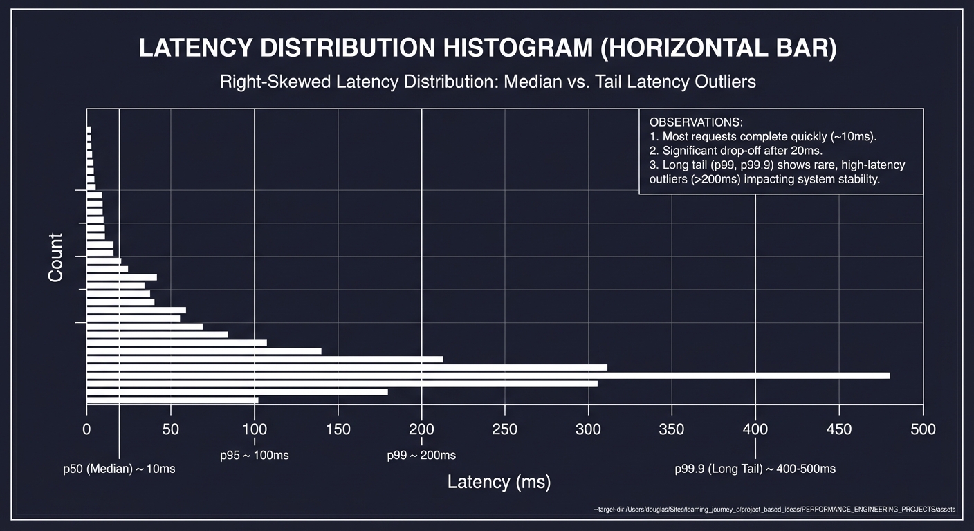
Latency Distribution Shapes

Real latency distributions are NOT normal. They have:

• Right skew: Long tail of slow requests
• Multi-modal: Peaks at different latency levels
• Heavy tails: Extreme outliers (10x, 100x median)

Typical latency distribution:
Count
  │
  │ ▄
  │ ██
  │ ███
  │ ████
  │ █████
  │ ██████
  │ ███████▄
  │ █████████▄▄▄▄▄▄▄▄▄▄▄▄▄▄▄▄▄▄______.......
  └───────────────────────────────────────────→ Latency
    p50     p90  p95    p99        p99.9

Note the long tail extending far beyond median

Latency Budget Concept

A latency budget allocates time across components:

Total SLA: 100ms
├── Network (client→server): 10ms
├── Load balancer: 2ms
├── Authentication: 5ms
├── Business logic: 30ms
├── Database query: 40ms
├── Response serialization: 5ms
├── Network (server→client): 8ms
└── Buffer for variance: 0ms ← PROBLEM!

Without buffer, any variance exceeds SLA. A realistic budget:

Total SLA: 100ms
├── Core processing: 50ms (50% of budget)
├── I/O operations: 30ms (30% of budget)
└── Variance buffer: 20ms (20% of budget)

---

Complete Project Specification

What You’re Building

A latency simulation and analysis toolkit called latency_sim that:

1. Generates synthetic workloads with configurable latency patterns
2. Simulates queuing effects at various load levels
3. Produces latency histograms suitable for observability export
4. Identifies latency budget violations and sources
5. Models mitigation strategies (timeouts, hedging, retry)

Functional Requirements

latency_sim run --workload <name> --qps <rate> --duration <sec>
latency_sim analyze --input <data.csv> --percentiles 50,90,95,99,99.9
latency_sim histogram --input <data.csv> --buckets <list> --output <file>
latency_sim budget --components <config.yaml> --sla <ms>
latency_sim mitigation --strategy <hedge|timeout|retry> --compare

Example Output

Latency Simulation Report
═══════════════════════════════════════════════════
Workload: web_api
Configuration:
  Target QPS: 500
  Duration: 300 seconds
  Total requests: 150,000

Latency Distribution:
───────────────────────────────────────────────────
  p50:    4.8 ms  ████████████████
  p75:    7.3 ms  ███████████████████████
  p90:   12.1 ms  ██████████████████████████████
  p95:   18.4 ms  ████████████████████████████████████
  p99:   38.9 ms  ████████████████████████████████████████████
  p99.9: 127.3 ms ████████████████████████████████████████████████████████████

Histogram (Prometheus-compatible):
───────────────────────────────────────────────────
  latency_bucket{le="5"}     68,421
  latency_bucket{le="10"}    24,832
  latency_bucket{le="25"}     5,127
  latency_bucket{le="50"}     1,384
  latency_bucket{le="100"}      198
  latency_bucket{le="250"}       38
  latency_count              150,000
  latency_sum                1,247,342

Budget Analysis (SLA: 50ms):
───────────────────────────────────────────────────
Component         Actual p99   Budget   Status
network_ingress   3.2 ms       5 ms     ✓ OK
authentication    4.8 ms       5 ms     ✓ OK
business_logic    22.1 ms      20 ms    ⚠ OVER (110%)
database          18.4 ms      15 ms    ⚠ OVER (123%)
serialization     2.1 ms       5 ms     ✓ OK
TOTAL            50.6 ms       50 ms    ✗ SLA VIOLATED

Tail Latency Analysis:
───────────────────────────────────────────────────
• p99 is 8.1x higher than p50 (tail amplification)
• 1,500 requests exceeded SLA (1%)
• Worst-case latency: 312 ms (65x p50)
• Queue depth exceeded 20 for 42 seconds (14%)

Root Cause Indicators:
───────────────────────────────────────────────────
• Database p99 correlates with queue depth spikes
• 89% of SLA violations occurred during high queue depth
• Recommendation: Reduce database query latency or add capacity

---

Solution Architecture

Component Design

┌─────────────────────────────────────────────────────────────┐
│                    CLI Interface                             │
│   Workload configuration, analysis parameters                │
└──────────────────────────┬──────────────────────────────────┘
                           │
          ┌────────────────┼────────────────┐
          │                │                │
          ▼                ▼                ▼
   ┌─────────────┐  ┌─────────────┐  ┌─────────────┐
   │ Workload    │  │ Queue       │  │ Timer       │
   │ Generator   │  │ Simulator   │  │ Engine      │
   └──────┬──────┘  └──────┬──────┘  └──────┬──────┘
          │                │                │
          └────────────────┼────────────────┘
                           │
                           ▼
           ┌───────────────────────────────┐
           │      Measurement Collector     │
           │  Per-request latency storage   │
           └───────────────┬───────────────┘
                           │
          ┌────────────────┼────────────────┐
          │                │                │
          ▼                ▼                ▼
   ┌─────────────┐  ┌─────────────┐  ┌─────────────┐
   │ Histogram   │  │ Percentile  │  │ Budget      │
   │ Builder     │  │ Calculator  │  │ Analyzer    │
   └─────────────┘  └─────────────┘  └─────────────┘

Key Data Structures

// Single request measurement
typedef struct {
    uint64_t request_id;
    uint64_t arrival_time_ns;
    uint64_t start_time_ns;      // When processing started
    uint64_t end_time_ns;
    uint64_t queue_depth;        // Queue depth at arrival
    // Component breakdown (optional)
    uint64_t component_times[MAX_COMPONENTS];
} request_record_t;

// Histogram for percentile calculation
typedef struct {
    double *bucket_bounds;       // [5, 10, 25, 50, 100, 250, 500, 1000]
    uint64_t *bucket_counts;
    size_t num_buckets;
    uint64_t total_count;
    double sum;                  // For mean calculation
} histogram_t;

// Latency budget configuration
typedef struct {
    const char *component_name;
    double budget_ms;
    double actual_p99_ms;
    double utilization;          // actual/budget
    int exceeded;
} budget_component_t;

typedef struct {
    budget_component_t *components;
    size_t num_components;
    double sla_ms;
    double total_actual_ms;
    int sla_violated;
} budget_analysis_t;

Workload Generator

// Simulates realistic latency distribution
double generate_latency(workload_config_t *config) {
    // Base latency (log-normal distribution for realism)
    double base = config->base_latency_ms;
    double variance = config->variance_factor;

    // Log-normal gives right-skewed distribution
    double normal = random_normal(0, 1);
    double latency = base * exp(variance * normal);

    // Add occasional spikes (GC, I/O contention)
    if (random_uniform() < config->spike_probability) {
        latency += config->spike_latency_ms;
    }

    return latency;
}

// Queue simulation
double simulate_queue_delay(queue_t *q, double service_time) {
    double arrival_time = current_time();

    // Find when queue will be free
    double queue_free_time = q->busy_until;
    double wait_time = (queue_free_time > arrival_time)
                       ? (queue_free_time - arrival_time)
                       : 0;

    // Update queue state
    q->busy_until = fmax(arrival_time, queue_free_time) + service_time;
    q->depth = (int)(wait_time / service_time);  // Approximate depth

    return wait_time;
}

---

Phased Implementation Guide

Phase 1: Basic Latency Collection (Days 1-3)

Goal: Measure and store per-request latencies.

Steps:

1. Create request record structure
2. Implement nanosecond-precision timing
3. Generate synthetic workload with sleep-based delays
4. Store latencies in array for analysis
5. Calculate basic statistics (min, max, mean)

Validation: Mean matches expected average latency.

Phase 2: Percentile Calculation (Days 4-5)

Goal: Accurate percentile computation.

Steps:

1. Implement array-based percentile calculation (sort + index)
2. Add histogram-based approximate percentiles
3. Compare accuracy of both methods
4. Generate distribution visualization

Validation: Percentiles match expected for known distributions.

Phase 3: Queue Simulation (Days 6-8)

Goal: Model queuing effects on latency.

Steps:

1. Implement M/M/1 queue simulation
2. Generate arrivals with Poisson process
3. Track queue depth over time
4. Show latency explosion at high utilization

Validation: Matches theoretical queuing formula within 10%.

Phase 4: Budget Analysis (Days 9-11)

Goal: Component-level budget tracking.

Steps:

1. Parse budget configuration (YAML/JSON)
2. Simulate multi-component latency
3. Calculate per-component p99
4. Identify budget violations
5. Generate recommendations

Validation: Correctly identifies over-budget components.

Phase 5: Observability Export (Days 12-14)

Goal: Production-ready histogram export.

Steps:

1. Implement Prometheus histogram format
2. Add stable dimension tagging
3. Create Datadog distribution format
4. Test import into real observability platform

Validation: Metrics appear correctly in Grafana/Datadog.

---

Testing Strategy

Statistical Validation

1. Known distribution: Generate exponential, verify percentiles match theory
2. Queuing formula: Verify M/M/1 queue matches analytical results
3. Percentile accuracy: Compare histogram to exact sort-based calculation

Edge Cases

1. Zero-latency requests: Handle correctly
2. Extreme outliers: Don’t overflow or distort statistics
3. Empty periods: Handle gaps in traffic

Load Testing

1. Sustained load: Run for hours, verify no memory leaks
2. Burst traffic: Handle 10x normal load
3. Slow drain: Verify queue eventually empties

---

Common Pitfalls and Debugging

Pitfall 1: Timer Resolution Issues

Symptom: All latencies cluster at same value.

Cause: Timer resolution too coarse for measurements.

Solution:

// Use CLOCK_MONOTONIC for nanosecond precision
struct timespec ts;
clock_gettime(CLOCK_MONOTONIC, &ts);
uint64_t ns = ts.tv_sec * 1000000000ULL + ts.tv_nsec;

// Verify resolution
struct timespec res;
clock_getres(CLOCK_MONOTONIC, &res);
printf("Timer resolution: %ld ns\n", res.tv_nsec);

Pitfall 2: Histogram Bucket Misdesign

Symptom: Most latencies fall in one bucket.

Cause: Bucket boundaries don’t match distribution.

Solution:

// Exponential buckets cover wide range
// Good: [1, 2, 5, 10, 25, 50, 100, 250, 500, 1000, +Inf]
// Bad:  [10, 20, 30, 40, 50, 60, 70, 80, 90, 100, +Inf]

// Align with SLO boundaries
// If SLO is 100ms, have bucket at 100ms exactly

Pitfall 3: Coordinated Omission

Symptom: Latency looks better than reality.

Cause: When system is slow, fewer requests are sent, hiding latency.

Solution: Use “intended” vs “actual” arrival times:

// Coordinated omission affected (WRONG)
for (int i = 0; i < num_requests; i++) {
    uint64_t start = now();
    send_request();        // May block if server slow
    uint64_t end = now();
    record_latency(end - start);
}

// Corrected (RIGHT)
uint64_t intended_interval = 1000000000 / target_qps;
uint64_t next_intended = now();

for (int i = 0; i < num_requests; i++) {
    uint64_t actual_start = now();
    send_request();
    uint64_t end = now();

    // Include time waiting for previous requests
    record_latency(end - next_intended);

    next_intended += intended_interval;
}

Pitfall 4: Ignoring Warmup Period

Symptom: First percentiles are way off.

Cause: System not at steady state (cold caches, JIT warming).

Solution: Discard first N seconds or N requests.

---

Extensions and Challenges

Extension 1: Hedging Simulation

Implement hedging (send duplicate request after timeout):

// If no response in 10ms, send to second server
// Use whichever responds first
// Measure improvement in p99

Extension 2: Adaptive Load Shedding

Implement admission control:

• Track queue depth
• Reject requests when queue > threshold
• Measure trade-off: rejected requests vs tail latency

Extension 3: Distributed Tracing Integration

Add trace ID propagation:

• Generate span for each component
• Export to Jaeger/Zipkin format
• Correlate slow requests with traces

Challenge: Real Service Integration

Apply latency analysis to real service:

• Instrument actual HTTP endpoints
• Measure component latencies
• Compare simulation to reality
• Tune model parameters

---

Real-World Connections

Industry Patterns

1. Google’s Tail at Scale: Hedged requests, backup requests
2. Amazon’s p99 SLOs: Everything measured at p99, not average
3. Netflix’s Adaptive Load Shedding: Concurrency limits based on latency
4. LinkedIn’s Latency Budgets: Component-level tracking

Observability Best Practices (2025)

1. Store histograms, not aggregates: Enables accurate percentiles
2. Use stable dimensions only: Avoid high-cardinality tags
3. Align buckets with SLOs: Bucket at exact SLO boundary
4. Track queue depth alongside latency: Enables correlation

---

Self-Assessment Checklist

Before considering this project complete, verify:

• You can explain why p99 diverges from median
• You demonstrated queuing effects on latency
• Your histogram buckets are appropriately distributed
• You can identify budget violations by component
• Latency export is compatible with real observability platforms
• You understand and avoid coordinated omission
• You can recommend mitigation strategies

---

Resources

Essential Reading

• “Designing Data-Intensive Applications” by Kleppmann, Chapter 8
• “Systems Performance” by Gregg, Chapter 2
• “Site Reliability Engineering” (Google), Chapter 4

Papers

• “The Tail at Scale” (Google, 2013)
• “Fail at Scale” (Facebook, 2015)

Tools

• HdrHistogram: High dynamic range histogram library
• Prometheus: Histogram implementation
• Grafana: Visualization and SLO tracking