Performance Engineering Projects
Goal
After completing these projects, you will understand performance engineering as a full-stack discipline: how programs actually consume CPU cycles, memory bandwidth, cache capacity, and I/O time, and how to turn that understanding into measurable latency and throughput improvements.
You will internalize:
- How to profile reality: sampling vs tracing, perf events, flamegraphs, and how to interpret them without guessing
- How to debug performance bugs: GDB, core dumps, and post-mortem analysis of hot paths and stalls
- How hardware really behaves: cache hierarchies, branch prediction, SIMD lanes, and why micro-optimizations sometimes work and often do not
- How to optimize latency: tail latency, queuing effects, lock contention, and jitter sources
- How to validate improvements: benchmarking discipline, statistical rigor, and regression detection
By the end, you will be able to explain why a system is slow, prove it with data, and implement targeted changes that predictably move real performance metrics.
Foundational Concepts: The Five Pillars
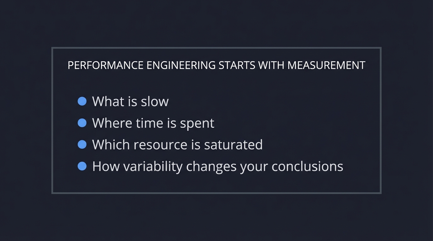
1. Measurement First — You Cannot Optimize What You Cannot Measure
┌─────────────────────────────────────────────────────────┐
│  PERFORMANCE ENGINEERING STARTS WITH MEASUREMENT       │
│                                                         │
│  You must know:                                         │
│  • What is slow                                          │
│  • Where time is spent                                   │
│  • Which resource is saturated                           │
│  • How variability changes your conclusions              │
└─────────────────────────────────────────────────────────┘
Modern Performance Engineering (2025)
In 2025, performance engineering combines traditional profiling with modern observability. Tools like perf, flamegraphs, and distributed tracing (Jaeger, Zipkin) work together. The key shift: performance is a system property, not just code quality.
Cloud-native systems track percentile latencies (p50, p95, p99) across distributed services, while on-premises systems focus on CPU cycles, cache misses, and throughput. Both require:
- Instrumentation: Histograms, not averages
- Baselines: Statistical significance testing
- Evidence: Flamegraphs and traces attached to every regression
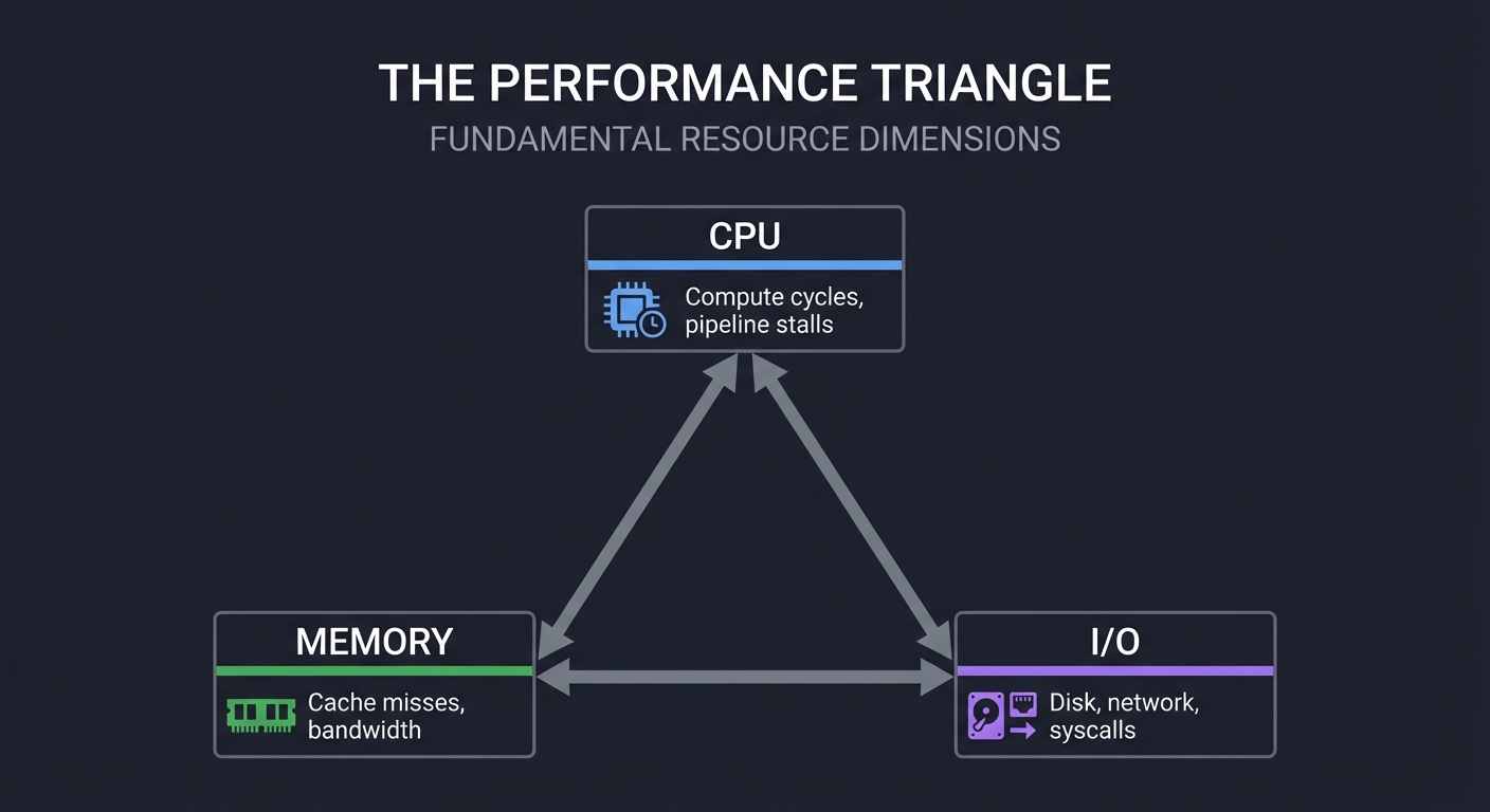
2. The Performance Triangle — CPU, Memory, I/O
        ┌───────────┐
        │    CPU    │  Compute cycles, pipeline stalls
        └─────┬─────┘
              │
              │
┌─────────────┼─────────────┐
│           MEMORY          │  Cache misses, bandwidth
└─────────────┼─────────────┘
              │
              │
        ┌─────┴─────┐
        │    I/O    │  Disk, network, syscalls
        └───────────┘
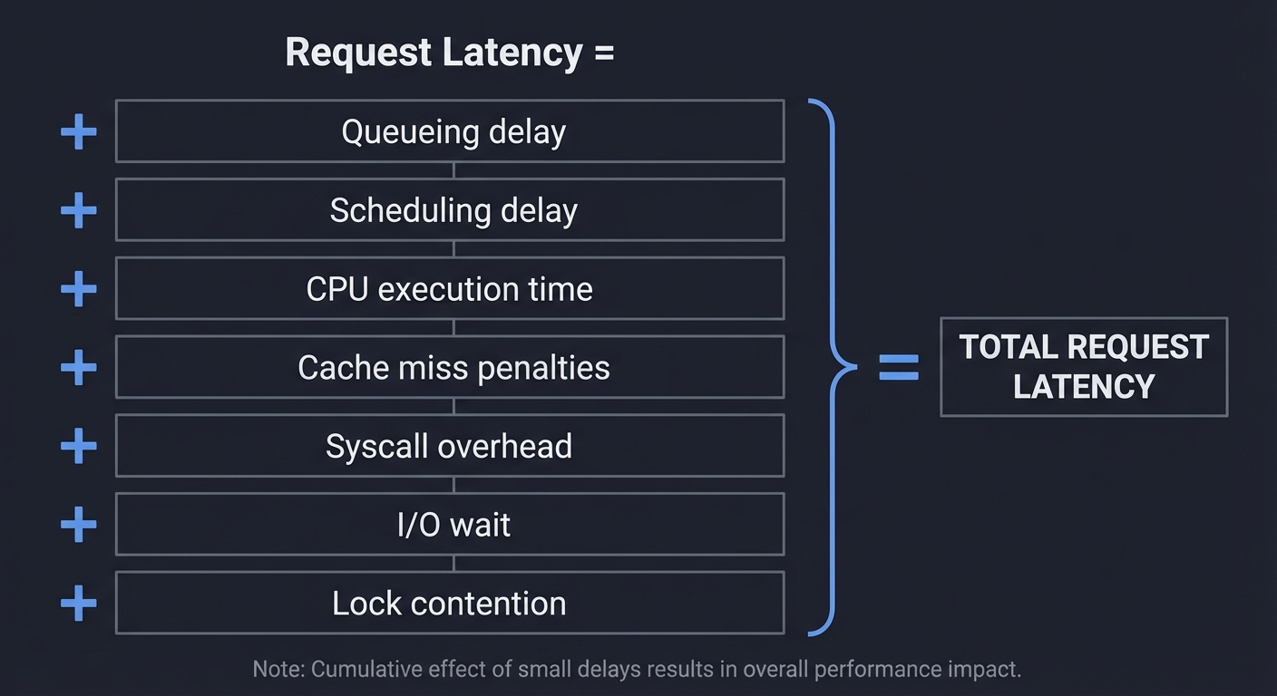
3. The Latency Stack — Why Small Delays Add Up
Request Latency =
  Queueing delay
+ Scheduling delay
+ CPU execution time
+ Cache miss penalties
+ Syscall overhead
+ I/O wait
+ Lock contention
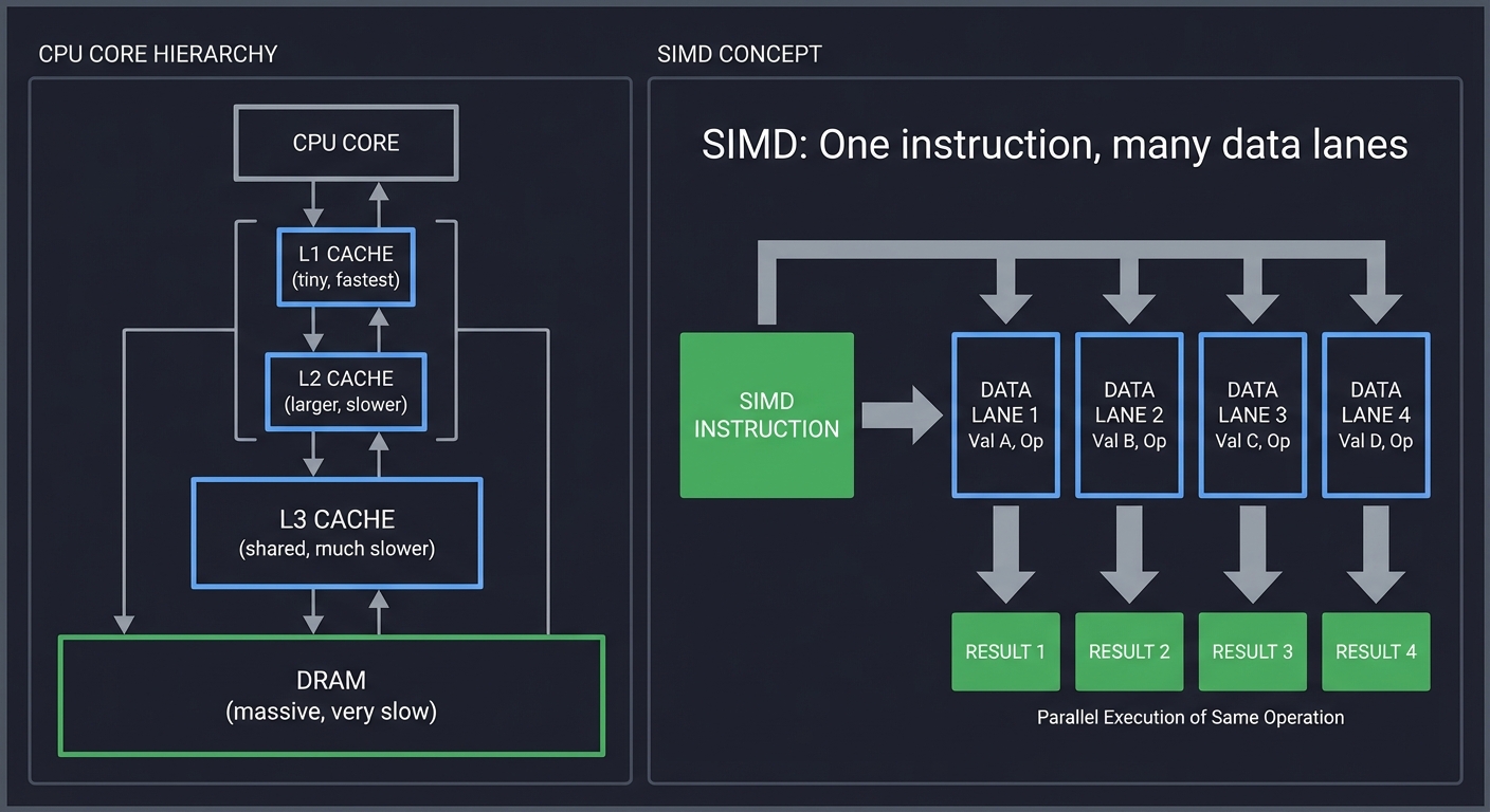
4. Hardware Reality — Caches, Pipelines, SIMD
CPU Core
  ├─ L1 Cache (tiny, fastest)
  ├─ L2 Cache (larger, slower)
  ├─ L3 Cache (shared, much slower)
  └─ DRAM (massive, very slow)

SIMD: One instruction, many data lanes
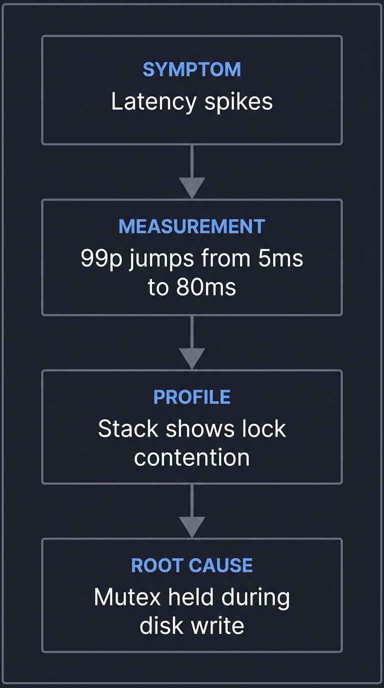
5. Debugging Performance — Finding the Real Cause
SYMPTOM: "Latency spikes"
  ↓
MEASUREMENT: "99p jumps from 5ms to 80ms"
  ↓
PROFILE: "Stack shows lock contention"
  ↓
ROOT CAUSE: "Mutex held during disk write"
Core Concept Analysis
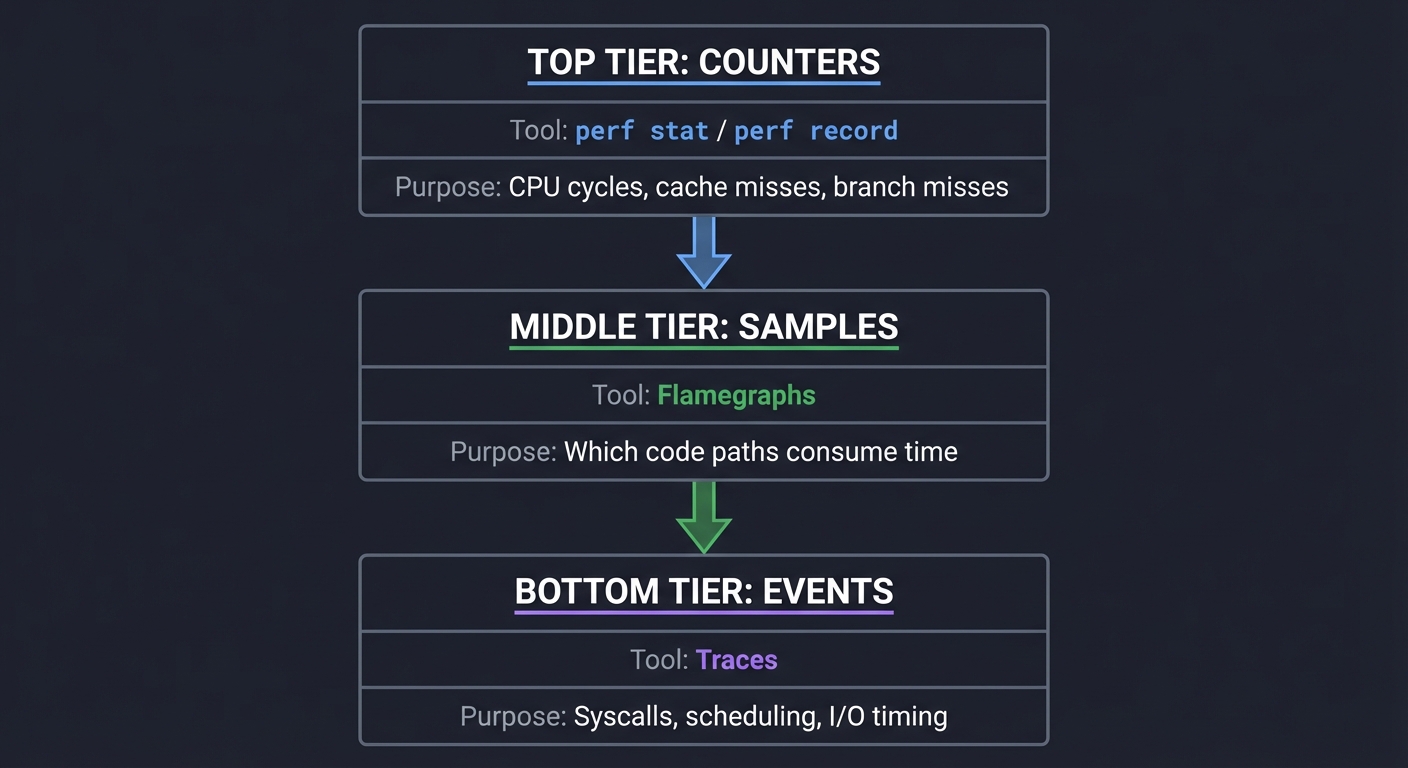
The Measurement Stack
┌───────────────┐   perf stat / perf record
│  Counters     │ → CPU cycles, cache misses, branch misses
└───────┬───────┘
        │
┌───────┴───────┐   Flamegraphs
│   Samples    │ → Which code paths consume time
└───────┬───────┘
        │
┌───────┴───────┐   Traces
│   Events     │ → Syscalls, scheduling, I/O timing
└───────────────┘
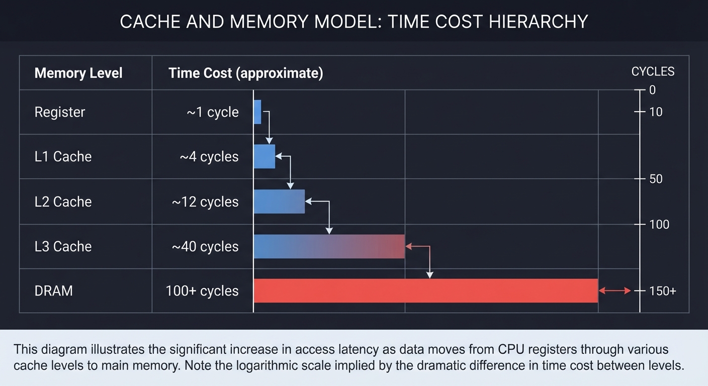
The Cache and Memory Model
Time Cost (approximate)
┌─────────────────────────────┐
│ Register        ~1 cycle    │
│ L1 Cache        ~4 cycles   │
│ L2 Cache        ~12 cycles  │
│ L3 Cache        ~40 cycles  │
│ DRAM            100+ cycles │
└─────────────────────────────┘
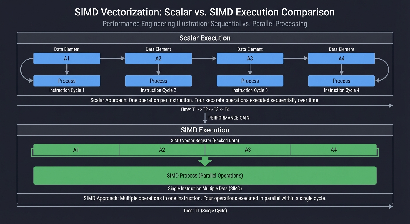
SIMD and Vectorization
Scalar:  A1 A2 A3 A4 -> one per instruction
SIMD:    [A1 A2 A3 A4] -> one instruction, 4 lanes
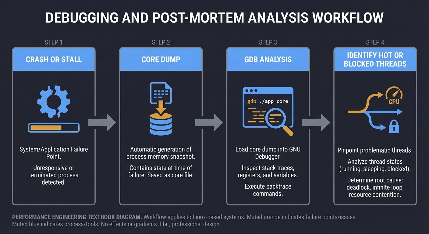
Debugging and Post-Mortem Analysis
Crash or stall -> Core dump -> GDB analysis -> Identify hot or blocked threads
Concept Summary Table
| Concept Cluster | What You Must Internalize |
|---|---|
| Measurement Discipline | You need repeatable benchmarks and correct statistics before trusting any optimization. |
| Profiling and Tracing | Sampling shows where time is spent; tracing shows why and when it happened. |
| CPU and Cache Behavior | Performance depends on cache locality, branch prediction, and memory access patterns. |
| SIMD and Vectorization | Wide data paths can multiply throughput, but only with aligned, predictable data. |
| Latency Engineering | Tail latency is a system property, not just a code property. |
| Debugging for Performance | GDB and core dumps can reveal blocked threads, stalls, and deadlocks. |
Deep Dive Reading By Concept
Concept 1: Measurement and Benchmarking
| Book | Chapter/Section | What You’ll Learn | Priority |
|---|---|---|---|
| “Systems Performance” by Brendan Gregg | Ch. 2: Methodology | How to structure a performance investigation | Essential |
| “High Performance Python” by Gorelick and Ozsvald | Ch. 1: Benchmarking | Measuring accurately and avoiding false conclusions | Recommended |
Concept 2: Profiling and Flamegraphs
| Book | Chapter/Section | What You’ll Learn | Priority |
|---|---|---|---|
| “Systems Performance” by Brendan Gregg | Ch. 6: CPUs | CPU profiling methods and tools | Essential |
| “Performance Analysis and Tuning on Modern CPUs” by Fog | Ch. 1-3: Microarchitecture | How microarchitecture affects profiling results | Recommended |
2025 Best Practices for Profiling:
- Use 99 Hz sampling (perf record -F 99) as standard - balances overhead with precision
- Always compile with debug symbols (-g flag) to get accurate stack traces
- Use differential flame graphs to compare performance between versions
- Modern profilers support over 100 implementations, but Brendan Gregg’s open-source FlameGraph toolkit remains the gold standard
Concept 3: Cache and Memory
| Book | Chapter/Section | What You’ll Learn | Priority |
|---|---|---|---|
| “Computer Systems: A Programmer’s Perspective” by Bryant and O’Hallaron | Ch. 6: Memory Hierarchy | Cache behavior and memory access patterns | Essential |
| “What Every Programmer Should Know About Memory” by Drepper | Sections 2-6 | Cache levels, bandwidth, and latency | Recommended |
Concept 4: SIMD and Vectorization
| Book | Chapter/Section | What You’ll Learn | Priority |
|---|---|---|---|
| “Computer Architecture: A Quantitative Approach” by Hennessy and Patterson | Ch. 3: Instruction-Level Parallelism | Vector units and throughput | Recommended |
| “Optimizing Software in C++” by Agner Fog | Ch. 10: Vectorization | SIMD principles and pitfalls | Essential |
2025 SIMD Performance Reality:
- Modern compilers with -O3 can auto-vectorize simple loops, reducing manual SIMD advantage
- Manual SIMD typically provides 2-4x speedup for suitable workloads (with optimization enabled)
- Cache-friendly data (1M elements): 3.8-4.0x speedup with SIMD
- Memory-bound data (1B elements): 2.0-2.1x speedup (bandwidth limited)
- Structure of Arrays (SoA) layout improves cache locality and enables better vectorization
- Focus on vectorizing the top 10% of hot loops for 70-80% of potential gains
Concept 5: Latency Engineering
| Book | Chapter/Section | What You’ll Learn | Priority |
|---|---|---|---|
| “Designing Data-Intensive Applications” by Kleppmann | Ch. 8: The Trouble with Distributed Systems | Tail latency and queuing | Recommended |
| “Site Reliability Engineering” by Beyer et al. | Ch. 4: Service Level Objectives | Latency targets and error budgets | Recommended |
2025 Latency Measurement Best Practices:
- Store latency as histograms, not rolled-up percentiles (Prometheus, Datadog support this)
- Tag metrics with stable dimensions only (method, route, status_code, region) - avoid user-specific labels
- Track request volume alongside percentiles - p99 with 20 requests means little
- Use ratio alerts: “P99 > 3 × P50 for 15m” to spot divergence
- Run benchmarks 5 times, drop worst, report mean of 4 to reduce noise from transient issues
- Approximately 20-30% of application failures relate to tail latency and queuing effects
Project List
Projects are ordered from foundational profiling to advanced hardware and latency optimization.
Project 1: “Performance Baseline Lab” — Measurement Discipline First
| Attribute | Value |
|---|---|
| Language | C (also: Rust, Go, C++) |
| Difficulty | Beginner |
| Time | Weekend |
| Knowledge Area | Benchmarking and Measurement |
| Tools | perf, time, taskset |
| Book | “Systems Performance” by Brendan Gregg |
What you’ll build: A repeatable benchmarking harness that measures runtime, variance, and CPU usage for a set of micro-tasks.
Why it teaches performance engineering: Without a reliable baseline, every optimization is a guess. This project forces you to build measurement discipline first.
Core challenges you’ll face:
- Designing repeatable workloads (maps to measurement methodology)
- Handling variance and noise (maps to statistics and sampling)
- Recording and comparing runs (maps to regression detection)
Key Concepts
- Benchmarking noise: “Systems Performance” - Brendan Gregg
- Measurement bias: “High Performance Python” - Gorelick and Ozsvald
- Repeatability: “The Practice of Programming” - Kernighan and Pike
Difficulty: Beginner Time estimate: Weekend Prerequisites: Basic C, command-line usage
Real World Outcome
You will have a CLI tool that runs a defined workload N times, reports min/median/99p duration, and stores results in a simple text report. When you run it, you will see a clear comparison between baseline and changed versions.
Example Output:
$ ./perf_lab run --workload "memcopy" --iters 100 --warmup 10
=================================================
Performance Baseline Report
=================================================
Workload:        memcopy (1MB buffer, aligned)
Date:            2025-01-27 14:32:15
CPU:             Intel Core i7-9700K @ 3.60GHz (pinned to core 2)
Frequency:       Fixed at 3.6GHz (turbo disabled)
Iterations:      100 (after 10 warmup runs)
-------------------------------------------------

Wall-clock time:
  Min:           12.234 ms
  Median:        12.891 ms
  Mean:          12.967 ms
  99th %ile:     14.782 ms
  Max:           15.201 ms
  Std Dev:       0.421 ms
  Coef Var:      3.25%

CPU Performance Counters (per run):
  Cycles:              46,408,192 (13.39 cycles/byte)
  Instructions:        87,234,561
  IPC:                 1.88
  L1-dcache-misses:    1,892,451 (0.054% miss rate)
  LLC-misses:          127,834 (0.004% miss rate)
  Branch-misses:       42,183 (0.12% of branches)
  Context-switches:    0
  Page-faults:         0

-------------------------------------------------
Recommendation: Variance is acceptable (CV < 5%).
                This baseline is suitable for comparison.

Report saved: reports/memcopy_baseline_2025-01-27.txt
Metrics saved:  reports/memcopy_baseline_2025-01-27.csv
After optimization, you can compare:
$ ./perf_lab compare reports/memcopy_baseline_2025-01-27.txt reports/memcopy_optimized_2025-01-27.txt

Change Detection Report
-------------------------------------------------
Median latency:    12.891 ms -> 9.234 ms  (-28.4%, p < 0.001) ✓ FASTER
99th %ile:         14.782 ms -> 10.123 ms (-31.5%, p < 0.001) ✓ FASTER
IPC:               1.88 -> 2.34 (+24.5%) ✓ IMPROVED
LLC-misses:        127,834 -> 89,234 (-30.2%) ✓ IMPROVED
-------------------------------------------------
Conclusion: Statistically significant improvement detected.
The Core Question You’re Answering
“How do I know if a change actually made performance better?”
Before you write any code, sit with this question. Most optimization efforts fail because there is no trustworthy baseline or measurement process.
Concepts You Must Understand First
Stop and research these before coding:
- Benchmarking discipline
- What makes a benchmark repeatable?
- How does CPU frequency scaling affect results?
- Why does warm-up matter?
- Book Reference: “Systems Performance” Ch. 2 - Brendan Gregg
- Variance and noise
- What are outliers and how do they distort averages?
- Why is p99 more informative than the mean for latency?
- Book Reference: “High Performance Python” Ch. 1 - Gorelick and Ozsvald
Questions to Guide Your Design
Before implementing, think through these:
- Workload definition
- How will you isolate CPU-bound vs memory-bound tasks?
- What inputs represent realistic sizes?
- How will you keep input stable across runs?
- Specific questions:
- Will you use a fixed seed for random data to ensure identical inputs across runs?
- How will you prevent the compiler from optimizing away your benchmark workload?
- Should you use volatile pointers or explicit memory barriers to force real memory accesses?
- What workload sizes will you test: L1-fit (32KB), L2-fit (256KB), L3-fit (8MB), DRAM (100MB+)?
- Metrics and reporting
- Which metrics are most meaningful for your workload?
- How will you store historical baselines?
- Specific questions:
- Will you track IPC (instructions per cycle) to detect micro-architectural bottlenecks?
- Should you record LLC (last-level cache) miss rates to identify memory bottlenecks?
- How will you store reports: plain text, CSV, JSON, or SQLite database?
- Will you implement automatic regression detection by comparing against rolling baseline?
- Should you track environment metadata (kernel version, CPU model, NUMA topology)?
- Controlling variance
- Specific questions:
- How will you disable address space layout randomization (ASLR) if needed?
- Will you run with elevated priority (nice -20) to reduce scheduler interference?
- Should you disable hyperthreading for more consistent results?
- How will you detect and warn about high variance (CV > 5%)?
- Specific questions:
Thinking Exercise
The Baseline Trap
Before coding, describe a scenario where an optimization appears faster but is actually noise. Write down three sources of variability (scheduler, CPU turbo, cache warmth) and how each could mislead your conclusion.
Describe: "Before" vs "After" results and why they are not comparable.
List: 3 variability sources and how you would control them.
Example Scenario to Think Through:
You run your baseline: median = 10.2ms (no CPU pinning, turbo enabled) You make a code change and run again: median = 9.8ms (-4% faster!) You declare victory… but is it real?
Variability Source 1: CPU Turbo Boost
- Problem: First run might have been thermally throttled, second run benefited from turbo boost
- Evidence: Check CPU frequency logs - first run at 2.8GHz, second at 4.2GHz
- Control: Disable turbo with
echo 1 > /sys/devices/system/cpu/intel_pstate/no_turbo - Expected outcome: After control, both runs measure 10.1ms - no real improvement
Variability Source 2: Scheduler Migration
- Problem: Process migrated between cores, causing cache flush and reload
- Evidence: High context-switch count in perf stat output
- Control: Use
taskset -c 2 ./benchto pin to single core - Expected outcome: Variance drops from CV=8% to CV=2%
Variability Source 3: Cache Warmth
- Problem: Second run reuses warm caches and branch predictor state from first run
- Evidence: LLC-misses differ by 10x between runs
- Control: Implement explicit warmup runs (10 iterations) that don’t count toward measurement
- Expected outcome: First measured run and last measured run have similar cache miss rates
Deep Dive Exercise: Run this experiment yourself:
- Run benchmark 50 times WITHOUT controls
- Calculate median and CV - likely CV > 10%
- Add CPU pinning - CV drops to ~7%
- Add frequency locking - CV drops to ~4%
- Add warmup runs - CV drops to ~2%
- Add kernel command line isolcpus=2 - CV drops to ~1%
Plot a histogram of your 50 runs at each stage. You should see the distribution narrow as you add controls.
The Interview Questions They’ll Ask
Prepare to answer these:
- “How do you design a trustworthy benchmark?”
- “Why is median better than mean for latency?”
- “What is p99 and why does it matter?”
- “How can CPU frequency scaling distort a benchmark?”
- “How do you detect regression over time?”
Hints in Layers
Hint 1: Starting Point Pick two micro-workloads: one CPU-bound (simple arithmetic loop), one memory-bound (array scan). Only then add metrics.
Concrete example workloads:
// CPU-bound: Integer arithmetic (should be L1-cache resident)
volatile uint64_t cpu_bound_work(size_t iterations) {
    uint64_t sum = 0;
    for (size_t i = 0; i < iterations; i++) {
        sum += i * 13 + 7;  // Prevent optimization
    }
    return sum;
}

// Memory-bound: Sequential array scan (exceeds L3 cache)
volatile uint64_t memory_bound_work(size_t size) {
    uint64_t *data = malloc(size);
    memset(data, 1, size);  // Fault in pages
    uint64_t sum = 0;
    for (size_t i = 0; i < size / sizeof(uint64_t); i++) {
        sum += data[i];  // Sequential access
    }
    free(data);
    return sum;
}
Hint 2: Next Level Run each workload multiple times with CPU pinned to a single core. Compare median and p99.
Concrete implementation:
#define ITERATIONS 100
#define WARMUP 10

// Use clock_gettime for nanosecond precision
struct timespec start, end;
double times[ITERATIONS];

// Warmup runs
for (int i = 0; i < WARMUP; i++) {
    volatile uint64_t result = cpu_bound_work(1000000);
}

// Measured runs
for (int i = 0; i < ITERATIONS; i++) {
    clock_gettime(CLOCK_MONOTONIC, &start);
    volatile uint64_t result = cpu_bound_work(1000000);
    clock_gettime(CLOCK_MONOTONIC, &end);

    times[i] = (end.tv_sec - start.tv_sec) * 1e9 +
               (end.tv_nsec - start.tv_nsec);
}

// Sort for percentiles
qsort(times, ITERATIONS, sizeof(double), compare_double);
double median = times[ITERATIONS / 2];
double p99 = times[(int)(ITERATIONS * 0.99)];
Run with CPU pinning:
taskset -c 2 ./perf_lab --workload cpu_bound
Hint 3: Technical Details Record both wall-clock time and CPU counters. Store results with timestamps for comparison.
Using perf_event_open for hardware counters:
#include <linux/perf_event.h>
#include <sys/syscall.h>

struct perf_event_attr pe;
memset(&pe, 0, sizeof(pe));
pe.type = PERF_TYPE_HARDWARE;
pe.size = sizeof(pe);
pe.config = PERF_COUNT_HW_CPU_CYCLES;
pe.disabled = 1;
pe.exclude_kernel = 1;

int fd = syscall(__NR_perf_event_open, &pe, 0, -1, -1, 0);
ioctl(fd, PERF_EVENT_IOC_RESET, 0);
ioctl(fd, PERF_EVENT_IOC_ENABLE, 0);

// Run workload
volatile uint64_t result = cpu_bound_work(1000000);

ioctl(fd, PERF_EVENT_IOC_DISABLE, 0);
long long count;
read(fd, &count, sizeof(count));
close(fd);

printf("CPU cycles: %lld
", count);
Hint 4: Tools/Debugging Use perf stat to validate your counters, then compare them to your stored reports.
Comprehensive perf stat command:
# Disable frequency scaling first
sudo cpupower frequency-set -g performance

# Run with full counter set
perf stat -e cycles,instructions,cache-references,cache-misses,branches,branch-misses,L1-dcache-loads,L1-dcache-load-misses,LLC-loads,LLC-load-misses,context-switches,page-faults taskset -c 2 ./perf_lab --workload memcopy --iters 100

# Expected output showing:
#   - IPC (instructions/cycles) should be 1.5-3.0 for compute-bound
#   - Cache miss rate < 1% for L1-fit workloads
#   - Zero context switches if properly pinned
#   - Zero page faults after warmup
Debugging high variance:
# Check if other processes interfering
ps aux --sort=-%cpu | head -10

# Monitor CPU frequency during benchmark
watch -n 0.1 'cat /proc/cpuinfo | grep MHz'

# Check thermal throttling
sensors | grep Core

# Verify CPU pinning worked
taskset -cp <pid>  # Should show: current affinity list: 2
Books That Will Help
| Topic | Book | Chapter |
|---|---|---|
| Benchmarking methodology | “Systems Performance” by Brendan Gregg | Ch. 2 |
| Measurement pitfalls | “High Performance Python” by Gorelick and Ozsvald | Ch. 1 |
| Debugging experiments | “The Practice of Programming” by Kernighan and Pike | Ch. 5 |
Project 2: “perf + Flamegraph Investigator” — Attribution of CPU Time
| Attribute | Value |
|---|---|
| Language | C (also: Rust, Go, C++) |
| Difficulty | Intermediate |
| Time | 1-2 weeks |
| Knowledge Area | Profiling and Flamegraphs |
| Tools | perf, flamegraph scripts |
| Book | “Systems Performance” by Brendan Gregg |
What you’ll build: A repeatable workflow that profiles a workload, generates flamegraphs, and annotates hotspots with causes.
Why it teaches performance engineering: Flamegraphs force you to attribute time to exact code paths, not guesses.
Core challenges you’ll face:
- Collecting reliable samples (maps to profiling fundamentals)
- Interpreting flamegraph width vs depth (maps to call stack attribution)
- Separating CPU time from I/O wait (maps to tracing vs sampling)
Key Concepts
- Profiling methodology: “Systems Performance” - Brendan Gregg
- Stack sampling: “Performance Analysis and Tuning on Modern CPUs” - Fog
- Flamegraph interpretation: Brendan Gregg blog (conceptual reference)
Difficulty: Intermediate Time estimate: 1-2 weeks Prerequisites: Project 1 complete, basic Linux tooling
Real World Outcome
You will produce a flamegraph report for a real workload and a short narrative of the top three hotspots and their likely causes. You will also have a repeatable command sequence for re-running the analysis after changes.
Example Output:
$ ./profile_run.sh --workload web_server --duration 30
=================================================
Flamegraph Profiling Report
=================================================
Workload:        web_server (1000 req/sec load)
Date:            2025-01-27 15:45:22
Duration:        30 seconds
Sampling freq:   99 Hz (system default, avoids lockstep with timers)
Total samples:   2,970
Debug symbols:   ✓ Available (compiled with -g -fno-omit-frame-pointer)
-------------------------------------------------

Profile captured: profiles/web_server_2025-01-27_154522.data
Flamegraph SVG:  reports/web_server_2025-01-27_154522.svg
Perf script:     reports/web_server_2025-01-27_154522.folded

Top CPU hotspots (by sample count):
1) parse_input              1,128 samples (38.0%)
   ├─ json_parse               687 samples (23.1%)
   ├─ validate_schema          298 samples (10.0%)
   └─ utf8_decode              143 samples (4.8%)

2) hash_lookup                624 samples (21.0%)
   ├─ hash_compute             374 samples (12.6%)
   └─ bucket_scan              250 samples (8.4%)

3) serialize_output           416 samples (14.0%)
   ├─ json_encode              312 samples (10.5%)
   └─ buffer_append            104 samples (3.5%)

4) malloc/free                297 samples (10.0%)
5) memcpy                     178 samples (6.0%)
-------------------------------------------------

Analysis:
✓ parse_input dominates at 38% - JSON parsing is the primary bottleneck
  → json_parse (23%) is the specific hot function
  → Consider: jemalloc for allocation-heavy parsing, or pre-allocated buffers

✓ hash_lookup (21%) - second hotspot
  → hash_compute (12.6%) suggests hash function itself is expensive
  → Consider: faster hash (xxHash, murmur3), or perfect hashing for known keys

✓ serialize_output (14%) - output formatting cost
  → json_encode dominates serialization
  → Consider: streaming serialization, or binary protocol (protobuf)

✓ malloc/free (10%) - memory allocation overhead visible
  → Scattered across call tree, indicates allocation pressure
  → Consider: memory pool, arena allocator, or tcmalloc

Recommendations:
1. Profile json_parse in isolation with perf record -g -F 999
2. Check if hash_compute has cache misses with perf stat -e cache-misses
3. Measure allocation rate with perf stat -e syscalls:sys_enter_brk,syscalls:sys_enter_mmap
Flamegraph visualization insights: The generated SVG shows:
- Width = CPU time: parse_input tower dominates the width
- Depth = call stack: deep stacks in json_parse indicate recursive descent parser
- Color = hot/warm: parse_input and children are colored red (hot)
- Tooltip data: Hover shows exact sample counts and percentages
After optimization (e.g., switching to simdjson):
$ ./profile_run.sh --workload web_server --duration 30

Top CPU hotspots (by sample count):
1) hash_lookup                892 samples (35.2%)  [was 21.0%, now primary bottleneck]
2) serialize_output           524 samples (20.7%)  [was 14.0%]
3) simdjson_parse             412 samples (16.3%)  [was json_parse at 23.1%]
4) malloc/free               198 samples (7.8%)   [was 10.0%]

Analysis:
✓ parse_input dropped from 38% to 16.3% - optimization successful!
✓ hash_lookup is now the primary bottleneck (35.2%)
  → Next optimization target identified
The Core Question You’re Answering
“Which specific functions are consuming the most CPU time, and why?”
Concepts You Must Understand First
Stop and research these before coding:
- Sampling vs tracing
- What does a sample represent?
- Why can sampling miss short functions?
- Book Reference: “Systems Performance” Ch. 6 - Brendan Gregg
- Call stacks and attribution
- How do stack frames map to time?
- What does a wide flamegraph bar mean?
- Book Reference: “Performance Analysis and Tuning on Modern CPUs” Ch. 1 - Fog
Questions to Guide Your Design
Before implementing, think through these:
- Profiling configuration
- What sample rate balances overhead vs accuracy?
- How will you ensure symbols are available for stacks?
- Interpreting results
- How will you differentiate hotspots that are expected from unexpected?
Thinking Exercise
The Misleading Hotspot
Describe a case where a function appears hot in a flamegraph, but optimizing it would not reduce total latency. Write down how you would verify whether it is truly the bottleneck.
Explain why a hotspot might be a symptom rather than a cause.
List two additional signals you would check.
The Interview Questions They’ll Ask
Prepare to answer these:
- “What is a flamegraph and what does width represent?”
- “How do you choose a sampling rate for perf?”
- “Why can a function appear hot but not be the real bottleneck?”
- “How do you separate CPU-bound work from I/O wait?”
- “What are the limitations of sampling profilers?”
Hints in Layers
Hint 1: Starting Point Profile a single workload from Project 1 to keep scope small.
Hint 2: Next Level Run multiple profiles and compare stability of hotspots.
Hint 3: Technical Details Use a separate step to symbolize and render flamegraphs so you can re-run without re-profiling.
Hint 4: Tools/Debugging Validate results with a second profiler to cross-check hotspots.
Books That Will Help
| Topic | Book | Chapter |
|---|---|---|
| CPU profiling | “Systems Performance” by Brendan Gregg | Ch. 6 |
| Microarchitecture basics | “Performance Analysis and Tuning on Modern CPUs” by Fog | Ch. 1-3 |
| Profiling practices | “Optimizing Software in C++” by Agner Fog | Ch. 2 |
Project 3: “GDB + Core Dump Performance Autopsy” — Post-Mortem Analysis
| Attribute | Value |
|---|---|
| Language | C (also: C++, Rust, Go) |
| Difficulty | Intermediate |
| Time | 1-2 weeks |
| Knowledge Area | Debugging and Post-Mortem Analysis |
| Tools | GDB, core dumps |
| Book | “The Linux Programming Interface” by Michael Kerrisk |
What you’ll build: A repeatable crash-and-stall investigation workflow using core dumps and GDB to identify blocked threads and hot loops.
Why it teaches performance engineering: Post-mortem analysis is essential when performance issues only happen in production.
Core challenges you’ll face:
- Capturing useful core dumps (maps to process state capture)
- Reading thread backtraces (maps to stack and scheduler awareness)
- Correlating stack state with latency symptoms (maps to root-cause analysis)
Key Concepts
- Core dump generation: “The Linux Programming Interface” - Kerrisk
- GDB backtrace reasoning: “Debugging with GDB” - FSF
- Thread states: “Operating Systems: Three Easy Pieces” - Arpaci-Dusseau
Difficulty: Intermediate Time estimate: 1-2 weeks Prerequisites: Project 1 complete, basic GDB usage
Real World Outcome
You will have a written post-mortem that identifies the exact thread and function responsible for a synthetic stall. You will also have a checklist for capturing core dumps and analyzing them in GDB.
Example Output:
$ ./autopsy.sh --core core.1234
Loaded core: core.1234
Threads: 8
Hot thread: TID 7
Top frame: lock_acquire
Evidence: 3 threads waiting on same mutex
Conclusion: contention in request queue
The Core Question You’re Answering
“How do I explain a performance incident when I cannot reproduce it?”
Concepts You Must Understand First
Stop and research these before coding:
- Core dumps and process state
- What is captured in a core dump?
- How do you map memory to symbols?
- Book Reference: “The Linux Programming Interface” Ch. 20 - Kerrisk
- Thread scheduling and blocking
- How do you identify blocked threads?
- What does a waiting thread look like in backtrace?
- Book Reference: “Operating Systems: Three Easy Pieces” Ch. 26 - Arpaci-Dusseau
Questions to Guide Your Design
Before implementing, think through these:
- Reproducible stall scenario
- What controllable condition will cause blocking?
- How will you capture a core at the right moment?
- Analysis workflow
- Which thread clues indicate a hot loop vs a lock wait?
Thinking Exercise
The Frozen System
Write a narrative of how you would distinguish between a CPU-bound loop and a thread deadlock using only a core dump and backtraces.
List the signals you would look for in stack traces and thread states.
The Interview Questions They’ll Ask
Prepare to answer these:
- “What is a core dump and how do you use it?”
- “How can you diagnose lock contention from a core dump?”
- “How do you identify a hot loop in GDB?”
- “What makes performance bugs hard to reproduce?”
- “How do you capture a core dump safely in production?”
Hints in Layers
Hint 1: Starting Point Create a workload that deliberately blocks on a lock and capture a core at peak stall.
Hint 2: Next Level Compare thread backtraces to see which thread is holding the lock and which are waiting.
Hint 3: Technical Details Use thread backtrace summaries to identify hot frames and blocked frames.
Hint 4: Tools/Debugging Write a short checklist for core capture, symbol loading, and triage steps.
Books That Will Help
| Topic | Book | Chapter |
|---|---|---|
| Core dumps | “The Linux Programming Interface” by Kerrisk | Ch. 20 |
| Debugging practice | “Debugging with GDB” by FSF | Ch. 7 |
| Thread states | “Operating Systems: Three Easy Pieces” by Arpaci-Dusseau | Ch. 26 |
Project 4: “Cache Locality Visualizer” — Data Layout Effects
| Attribute | Value |
|---|---|
| Language | C (also: C++, Rust, Zig) |
| Difficulty | Advanced |
| Time | 1-2 weeks |
| Knowledge Area | CPU Caches and Memory Access |
| Tools | perf, cachegrind (optional) |
| Book | “Computer Systems: A Programmer’s Perspective” |
What you’ll build: A set of experiments that visualize how data layout and access patterns change cache miss rates and runtime.
Why it teaches performance engineering: Cache behavior is often the biggest performance lever in real systems.
Core challenges you’ll face:
- Designing access patterns (maps to spatial and temporal locality)
- Measuring cache miss rates (maps to hardware counters)
- Connecting layout decisions to runtime impact (maps to memory hierarchy)
Key Concepts
- Memory hierarchy: “CS:APP” - Bryant and O’Hallaron
- Cache effects: “What Every Programmer Should Know About Memory” - Drepper
- Data layout: “Optimizing Software in C++” - Agner Fog
Difficulty: Advanced Time estimate: 1-2 weeks Prerequisites: Projects 1-2 complete, basic understanding of caches
Real World Outcome
You will produce a report with side-by-side timing and cache-miss data for different data layouts and access patterns, plus a short explanation of which pattern wins and why.
Example Output:
$ ./cache_lab report
Pattern A (row-major): 120 ms, L1 miss rate 2%
Pattern B (column-major): 940 ms, L1 miss rate 38%
Conclusion: stride access destroys cache locality
The Core Question You’re Answering
“Why does the same algorithm run 8x slower just by changing data layout?”
Concepts You Must Understand First
Stop and research these before coding:
- Cache hierarchy
- What is the cost difference between L1 and DRAM?
- How do cache lines work?
- Book Reference: “CS:APP” Ch. 6 - Bryant and O’Hallaron
- Locality
- What is spatial vs temporal locality?
- How does stride size affect misses?
- Book Reference: Drepper, Sections 2-3
Questions to Guide Your Design
Before implementing, think through these:
- Experiment design
- How will you isolate access patterns from computation cost?
- What data sizes cross cache boundaries?
- Measurement
- Which counters best indicate cache pressure?
Thinking Exercise
The Cache Line Walk
Draw a grid of memory addresses for a 2D array. Mark which cache lines are touched when traversing row-major vs column-major. Explain why one pattern reuses cache lines and the other does not.
Sketch: memory layout of a 4x4 array and show access order.
The Interview Questions They’ll Ask
Prepare to answer these:
- “What is a cache line and why does it matter?”
- “Explain spatial vs temporal locality.”
- “Why is column-major access slow in C for row-major arrays?”
- “How do you measure cache misses with perf?”
- “How can data layout dominate algorithmic complexity?”
Hints in Layers
Hint 1: Starting Point Start with a 2D array scan and compare two traversal orders.
Hint 2: Next Level Scale the array so it crosses L1, then L2, then L3 sizes.
Hint 3: Technical Details Record cache miss counters alongside runtime for each test.
Hint 4: Tools/Debugging Use perf stat with cache events to validate your assumptions.
Books That Will Help
| Topic | Book | Chapter |
|---|---|---|
| Memory hierarchy | “Computer Systems: A Programmer’s Perspective” | Ch. 6 |
| Cache behavior | “What Every Programmer Should Know About Memory” | Sections 2-4 |
| Data layout | “Optimizing Software in C++” by Agner Fog | Ch. 5 |
Project 5: “Branch Predictor and Pipeline Lab” — CPU Microarchitecture
| Attribute | Value |
|---|---|
| Language | C (also: C++, Rust, Zig) |
| Difficulty | Advanced |
| Time | 1-2 weeks |
| Knowledge Area | CPU Microarchitecture |
| Tools | perf, cpu topology tools |
| Book | “Computer Architecture: A Quantitative Approach” |
What you’ll build: A set of controlled experiments that show branch misprediction penalties and pipeline effects.
Why it teaches performance engineering: Branch mispredictions are invisible in code review but dominate CPU time.
Core challenges you’ll face:
- Creating predictable vs unpredictable branches (maps to branch prediction)
- Measuring misprediction rates (maps to hardware counters)
- Relating pipeline stalls to latency (maps to CPU execution)
Key Concepts
- Branch prediction: “Computer Architecture” - Hennessy and Patterson
- Pipeline stalls: “Performance Analysis and Tuning on Modern CPUs” - Fog
- CPU counters: “Systems Performance” - Brendan Gregg
Difficulty: Advanced Time estimate: 1-2 weeks Prerequisites: Projects 1-2 complete, basic CPU architecture
Real World Outcome
You will produce a report that shows how predictable branches run faster and how mispredictions increase cycles per instruction.
Example Output:
$ ./branch_lab report --iterations 100000000
=== Branch Prediction Benchmark Results ===

Pattern Analysis (100M iterations):
  Predictable branches (sorted data):
    Runtime: 124 ms
    Cycles per instruction (CPI): 0.82
    Branch misprediction rate: 0.4%
    Instructions per cycle (IPC): 3.21

  Unpredictable branches (random data):
    Runtime: 487 ms
    Cycles per instruction (CPI): 2.94
    Branch misprediction rate: 48.3%
    Instructions per cycle (IPC): 0.89
    Slowdown: 3.93x

Branch Patterns Tested:
  1. Sorted ascending:    0.3% mispredict, IPC 3.4
  2. Sorted descending:   0.3% mispredict, IPC 3.4
  3. Alternating (0,1,0,1): 1.2% mispredict, IPC 2.8
  4. Random 50/50:       49.8% mispredict, IPC 0.85
  5. Biased 90/10:       8.7% mispredict, IPC 2.1

Real-world Impact:
  - Sorted binary search: 15-20 cycles/iteration
  - Unsorted binary search: 45-60 cycles/iteration
  - Branchless code (cmov): 12-18 cycles/iteration (best for unpredictable)

Pipeline Analysis:
  - Misprediction penalty: 15-20 cycles on modern CPUs
  - Pipeline depth: 14-19 stages (Intel/AMD 2025)
  - Correctly predicted: ~1 cycle effective cost

Saved detailed report: reports/branch_analysis_2025-01-10.txt
Performance Numbers to Expect (2025 hardware):
- Predictable branches: Near-zero penalty, IPC 3-4
- Random branches (50/50): IPC drops to 0.8-1.2, 3-4x slowdown
- Misprediction cost: 15-20 cycles per miss on modern out-of-order CPUs
The Core Question You’re Answering
“Why does a tiny conditional statement slow down an entire loop?”
Concepts You Must Understand First
Stop and research these before coding:
- Branch prediction
- What does the CPU predict and when?
- What happens on misprediction?
- Book Reference: “Computer Architecture” Ch. 3 - Hennessy and Patterson
Concrete Example (Modern CPUs 2025):
- CPUs use two-level adaptive predictors that track branch history patterns
- Correctly predicted branch: Costs ~1 cycle (resolved in decode/execute stage)
- Mispredicted branch: Costs 15-20 cycles (must flush pipeline and restart)
- Branch Target Buffer (BTB): Caches target addresses for taken branches
Patterns that defeat predictors:
// GOOD: Predictable pattern (99%+ accuracy) for (i = 0; i < n; i++) { if (array[i] < threshold) { // Assumes sorted data sum += array[i]; } } // BAD: Random pattern (50% accuracy = coin flip) for (i = 0; i < n; i++) { if (rand() % 2) { // Completely unpredictable sum += array[i]; } } // SOLUTION: Branchless code for unpredictable data for (i = 0; i < n; i++) { int mask = -(array[i] < threshold); // -1 if true, 0 if false sum += array[i] & mask; // No branch, uses CMOV instruction } - Pipeline execution
- How do pipeline stalls reduce throughput?
- Book Reference: “Performance Analysis and Tuning on Modern CPUs” Ch. 2 - Fog
Concrete Example (Intel/AMD 2025 CPUs):
- Pipeline depth: 14-19 stages (fetch, decode, rename, schedule, execute, retire)
- Out-of-order execution: CPU can execute ~200+ instructions simultaneously
- Misprediction impact: Flushes all speculative work in pipeline
The Math:
With 50% branch misprediction rate:
- 50% of branches: 1 cycle (correct prediction)
- 50% of branches: 18 cycles (misprediction penalty)
- Average cost: (0.5 × 1) + (0.5 × 18) = 9.5 cycles per branch

With 99% branch prediction rate:
- 99% of branches: 1 cycle
- 1% of branches: 18 cycles
- Average cost: (0.99 × 1) + (0.01 × 18) = 1.17 cycles per branch

Speedup from predictability: 9.5 / 1.17 = 8.1x
Questions to Guide Your Design
Before implementing, think through these:
- Experiment design
- How will you control input distributions to change predictability?
- How will you isolate branch cost from memory cost?
- Metrics
- Which counters best indicate misprediction impact?
Thinking Exercise
The Pipeline Flush
Before coding, trace through the exact sequence of events during a branch misprediction:
Scenario: A modern CPU with 16-stage pipeline executing this code:
for (int i = 0; i < n; i++) {
    if (data[i] > threshold) {  // Branch at address 0x1000
        result += data[i] * 2;  // Target: 0x1008
    }
    count++;  // Fall-through: 0x1010
}
Pipeline Stages:
Cycle 1:  Fetch branch instruction (0x1000)
Cycle 2:  Decode branch, predict TAKEN (based on history)
Cycle 3:  Speculatively fetch from 0x1008 (target)
Cycle 4:  Decode target instructions
Cycle 5:  Execute target instructions
...
Cycle 7:  Branch condition evaluated -> PREDICTION WAS WRONG!
What happens on misprediction:
Cycle 7:  Detect misprediction
Cycle 8:  FLUSH all speculative work (cycles 3-7 wasted)
Cycle 9:  Restart fetch from correct address (0x1010)
Cycle 10: Decode correct path
...
Cycle 24: Finally complete the correct instruction

Cost: 17 cycles wasted (7 for speculation + 10 to refill pipeline)
Your Task:
1. Calculate the throughput impact:
   - Loop has 1 branch every 5 instructions
   - With 50% misprediction rate, what is the effective CPI?
   - With 99% prediction rate, what is the effective CPI?

2. Explain why sorted data has ~0% misprediction:
   - What pattern does the predictor learn?
   - Why does this pattern repeat reliably?

3. Design a workload that would defeat even adaptive predictors:
   - What sequence breaks pattern detection?
The Interview Questions They’ll Ask
Prepare to answer these:
- “What is branch prediction and why does it matter?”
- “What is a pipeline stall?”
- “How does misprediction affect CPI?”
- “How do you measure branch misses in perf?”
- “When does branch prediction not matter?”
Hints in Layers
Hint 1: Starting Point Create two loops with identical work but different branch predictability:
// Test 1: Sorted data (highly predictable)
int sum = 0;
for (int i = 0; i < n; i++) {
    if (sorted_array[i] > threshold) sum += sorted_array[i];
}

// Test 2: Random data (unpredictable)
int sum = 0;
for (int i = 0; i < n; i++) {
    if (random_array[i] > threshold) sum += random_array[i];
}
Compile with -O2 (not -O3, which may optimize away branches).
Hint 2: Next Level Use perf to measure branch prediction accuracy and CPI:
# Measure branch mispredictions
perf stat -e branches,branch-misses,instructions,cycles ./branch_lab sorted
perf stat -e branches,branch-misses,instructions,cycles ./branch_lab random

# Expected results:
# Sorted: branch-misses/branches < 1%, CPI ~ 0.8-1.2
# Random: branch-misses/branches ~ 45-50%, CPI ~ 2.5-3.5
Hint 3: Technical Details Isolate branch effects from memory effects:
# Pin to single CPU core to avoid context switches
taskset -c 0 ./branch_lab

# Ensure data fits in L3 cache to avoid DRAM latency
# L3 typically 8-32 MB, so use arrays < 8 MB

# Disable CPU frequency scaling for consistent results
sudo cpupower frequency-set --governor performance

# Compile with specific flags to control optimization:
gcc -O2 -march=native -fno-unroll-loops -o branch_lab branch_lab.c
Hint 4: Tools/Debugging Comprehensive perf command for branch analysis:
# Intel CPUs (2025)
perf stat -e branches,branch-misses,branch-loads,branch-load-misses \
          -e cpu-cycles,instructions,cache-references,cache-misses \
          -e stalled-cycles-frontend,stalled-cycles-backend \
          -r 10 ./branch_lab

# AMD CPUs (2025)
perf stat -e retired_branches,retired_branches_misp,retired_instructions \
          -e cycles,l1d_cache_accesses,l1d_cache_misses \
          -r 10 ./branch_lab

# Analyze assembly to verify no loop unrolling or vectorization:
objdump -d branch_lab | less
# Look for predictable branch patterns in hot loop
Hint 5: Expected Performance Counters For sorted (predictable) vs random (unpredictable) patterns:
Sorted/Predictable:
  Branch misprediction rate: 0.3-1%
  Cycles per instruction (CPI): 0.8-1.2
  Instructions per cycle (IPC): 2.5-3.5
  Stalled cycles: < 10%

Random/Unpredictable:
  Branch misprediction rate: 45-50%
  Cycles per instruction (CPI): 2.5-3.5
  Instructions per cycle (IPC): 0.8-1.2
  Stalled cycles: > 60% (waiting on branch resolution)

Performance degradation: 3-4x slowdown from mispredictions
Hint 6: Branchless Alternative Test branchless code for comparison:
// Branchless version using conditional move (CMOV)
for (int i = 0; i < n; i++) {
    int mask = -(array[i] > threshold);  // -1 or 0
    sum += array[i] & mask;
}

// Compile and verify CMOV is used:
gcc -O2 -march=native -S branch_lab.c
grep cmov branch_lab.s  // Should see cmovg, cmovl, etc.
Books That Will Help
| Topic | Book | Chapter |
|---|---|---|
| Branch prediction | “Computer Architecture” by Hennessy and Patterson | Ch. 3 |
| Pipeline stalls | “Performance Analysis and Tuning on Modern CPUs” by Fog | Ch. 2 |
| CPU counters | “Systems Performance” by Brendan Gregg | Ch. 6 |
Project 6: “SIMD Throughput Explorer” — Vectorization Speedups
| Attribute | Value |
|---|---|
| Language | C (also: C++, Rust, Zig) |
| Difficulty | Expert |
| Time | 1 month+ |
| Knowledge Area | SIMD and Vectorization |
| Tools | perf, compiler vectorization reports |
| Book | “Optimizing Software in C++” by Agner Fog |
What you’ll build: A set of experiments showing scalar vs SIMD throughput for numeric workloads.
Why it teaches performance engineering: SIMD is one of the most powerful (and misunderstood) sources of speedup.
Core challenges you’ll face:
- Structuring data for vectorization (maps to alignment and layout)
- Measuring speedup correctly (maps to measurement discipline)
- Handling edge cases where SIMD fails (maps to control flow divergence)
Key Concepts
- SIMD fundamentals: “Optimizing Software in C++” - Agner Fog
- Vector units: “Computer Architecture” - Hennessy and Patterson
- Alignment: “CS:APP” - Bryant and O’Hallaron
Difficulty: Expert Time estimate: 1 month+ Prerequisites: Projects 1,2,4 complete; basic CPU architecture
Real World Outcome
You will produce a side-by-side report showing the throughput difference between scalar and vectorized workloads, with evidence of alignment and data layout effects.
Example Output:
$ ./simd_lab report
Scalar: 1.0x baseline
SIMD:   3.7x speedup
Aligned data: 4.2x speedup
Unaligned data: 2.1x speedup
The Core Question You’re Answering
“When does SIMD actually speed things up, and when does it not?”
Concepts You Must Understand First
Stop and research these before coding:
- Vectorization basics
- What is a SIMD lane?
- What data sizes match vector width?
- Book Reference: “Optimizing Software in C++” Ch. 10 - Fog
- Alignment and layout
- Why does alignment matter for vector loads?
- Book Reference: “CS:APP” Ch. 6 - Bryant and O’Hallaron
Questions to Guide Your Design
Before implementing, think through these:
- Data preparation
- How will you ensure contiguous, aligned data?
- Measurement
- How will you isolate compute from memory bottlenecks?
Thinking Exercise
The SIMD Mismatch
Describe a dataset where SIMD would not help due to irregular memory access. Explain how you would detect that in a profiler.
List the symptoms of non-vectorizable workloads.
The Interview Questions They’ll Ask
Prepare to answer these:
- “What is SIMD and why does it help?”
- “How does alignment affect SIMD performance?”
- “What workloads are good candidates for vectorization?”
- “How do you validate a claimed SIMD speedup?”
- “Why might SIMD not help even if the CPU supports it?”
Hints in Layers
Hint 1: Starting Point Start with a simple numeric loop and compare scalar vs vectorized versions conceptually.
Hint 2: Next Level Measure with large enough data to avoid timing noise.
Hint 3: Technical Details Separate aligned vs unaligned data experiments.
Hint 4: Tools/Debugging Use compiler reports to confirm vectorization decisions.
Books That Will Help
| Topic | Book | Chapter |
|---|---|---|
| SIMD fundamentals | “Optimizing Software in C++” by Agner Fog | Ch. 10 |
| Vector units | “Computer Architecture” by Hennessy and Patterson | Ch. 3 |
| Alignment | “Computer Systems: A Programmer’s Perspective” | Ch. 6 |
Project 7: “Latency Budget and Tail Latency Simulator” — Understanding p99
| Attribute | Value |
|---|---|
| Language | C (also: Go, Rust, Python) |
| Difficulty | Intermediate |
| Time | 1-2 weeks |
| Knowledge Area | Latency Engineering |
| Tools | perf, tracing tools |
| Book | “Designing Data-Intensive Applications” by Kleppmann |
What you’ll build: A workload simulator that produces latency distributions and demonstrates how small delays create large p99 spikes.
Why it teaches performance engineering: It connects micro-level delays to system-level tail latency.
Core challenges you’ll face:
- Modeling queueing delay (maps to latency distributions)
- Measuring p95/p99 (maps to statistics)
- Correlating spikes with system events (maps to tracing)
Key Concepts
- Tail latency: “Designing Data-Intensive Applications” - Kleppmann
- Queuing effects: “Systems Performance” - Gregg
- Latency metrics: “Site Reliability Engineering” - Beyer et al.
Difficulty: Intermediate Time estimate: 1-2 weeks Prerequisites: Project 1 complete, basic statistics
Real World Outcome
You will produce a CLI tool that generates latency histograms, exports metrics for observability platforms (Prometheus, Datadog), and demonstrates how queue depth affects tail latency under realistic load patterns.
Example Output:
$ ./latency_sim run --workload web_api --duration 300s --qps 500
Running workload: web_api (target: 500 QPS, duration: 300s)
Benchmark methodology: 5 runs, drop worst, report mean of remaining 4

Run 1: p99=42.1ms [dropped - outlier]
Run 2: p99=38.7ms
Run 3: p99=39.2ms
Run 4: p99=38.4ms
Run 5: p99=39.5ms

Final Results (mean of runs 2-5):
━━━━━━━━━━━━━━━━━━━━━━━━━━━━━━━━━━━━━━━━━━━━━
Latency Distribution (stored as histogram):
  p50:  4.8 ms  ████████████████
  p75:  7.3 ms  ███████████████████████
  p90:  12.1 ms ██████████████████████████████
  p95:  18.4 ms ████████████████████████████████████
  p99:  38.9 ms ████████████████████████████████████████████████████████
  p99.9: 127.3 ms ████████████████████████████████████████████████████████████████████

Histogram buckets (for Prometheus/Datadog):
  ≤5ms:    68,421 requests
  ≤10ms:   24,832 requests
  ≤25ms:    5,127 requests
  ≤50ms:    1,384 requests
  ≤100ms:     198 requests
  ≤250ms:      38 requests

Latency divergence detected:
  ⚠ p99 > 3 × p50 for 15m (SLO alert triggered at 14:23-14:38)
  Root cause: queue depth burst from 2 → 47 during periodic fsync

Queue depth correlation:
  Avg queue depth: 1.8
  Max queue depth: 47 (at p99.9 event)
  Queue saturation periods: 8 (total 127s / 300s = 42%)

Prometheus metrics exported to: ./metrics/latency_sim_2025-01-15.prom
Datadog histogram tags: {workload:web_api, stable_dimension:region_us_east}

Performance insight:
  Tail latency (p99) explodes 8x above median due to queuing.
  Under 80%+ utilization, every 1ms delay cascades into 10ms+ p99 spike.

Next steps:
  1. Add admission control to cap queue depth at 10
  2. Batch fsync operations to reduce periodic spikes
  3. Set SLO: p99 < 3 × p50 sustained over 15m window
Histogram Storage Best Practice (2025):
- Store latency as histograms with predefined buckets, not rolled-up percentiles
- Tag with stable dimensions only (region, service) - NEVER tag with high-cardinality values (user_id, request_id)
- Export in Prometheus histogram format or Datadog distribution format
- Keep bucket boundaries aligned with your SLO boundaries (e.g., if SLO is <50ms, have buckets at 10, 25, 50, 100, 250)
The Core Question You’re Answering
“Why does p99 explode even when average latency looks fine?”
Concepts You Must Understand First
Stop and research these before coding:
- Latency percentiles
- Why are percentiles more useful than averages?
- Book Reference: “Site Reliability Engineering” Ch. 4 - Beyer et al.
- Queueing theory basics
- What happens as utilization approaches 100%?
- Book Reference: “Systems Performance” Ch. 2 - Gregg
Questions to Guide Your Design
Before implementing, think through these:
- Workload shaping
- How will you generate bursts of load?
- How will you log queue depth over time?
- Visualization
- How will you present the latency distribution clearly?
Thinking Exercise
The Slow Tail
Describe a system where 1 percent of requests take 10x longer. Explain how that affects user experience and system capacity.
Write a short narrative with numbers (median, 95p, 99p).
The Interview Questions They’ll Ask
Prepare to answer these:
- “What is tail latency and why is it important?”
- “Why does queueing cause nonlinear latency growth?”
- “How do you measure and report p99?”
- “What are common sources of latency spikes?”
- “How do you reduce tail latency without overprovisioning?”
Hints in Layers
Hint 1: Starting Point Generate a steady workload and measure p50 and p99.
Hint 2: Next Level Introduce periodic bursts and observe the p99 jump.
Hint 3: Technical Details Record queue depth alongside latency metrics for correlation.
Hint 4: Tools/Debugging Use tracing to identify which stage introduces the long tail.
Books That Will Help
| Topic | Book | Chapter |
|---|---|---|
| Regression workflows | “Systems Performance” by Brendan Gregg | Ch. 2 |
| Benchmarking statistics | “High Performance Python” by Gorelick and Ozsvald | Ch. 1 |
| Profiling tooling | “Performance Analysis and Tuning on Modern CPUs” by Fog | Ch. 1-3 |
| Statistical testing | “Statistics for Experimenters” by Box, Hunter, and Hunter | Ch. 1-3 |
| CI/CD integration | “Accelerate” by Forsgren, Humble, and Kim | Ch. 4 |
| Performance budgets | “Site Reliability Engineering” by Beyer et al. | Ch. 4 |
| Regression detection | “The Art of Computer Systems Performance Analysis” by Jain | Ch. 13 |
Essential Reading for Performance Regression Detection:
- “Systems Performance” (2nd Edition) by Brendan Gregg - Ch. 2 covers methodology for performance analysis, including how to establish baselines and detect anomalies
- “High Performance Python” by Gorelick and Ozsvald - Ch. 1 provides practical guidance on benchmarking and statistical analysis
- “Statistics for Experimenters” by Box, Hunter, and Hunter - Essential for understanding statistical significance testing
- “The Art of Computer Systems Performance Analysis” by Raj Jain - Ch. 13 covers comparing systems and detecting performance differences
Additional Resources:
- Brendan Gregg’s Blog: Articles on flamegraph differential analysis and regression detection
- “Accelerate” DevOps book: CI/CD integration patterns for automated performance testing
-
“Site Reliability Engineering” (SRE Book): Performance budgets and SLO-based alerting
Project 8: “Lock Contention and Concurrency Profiler” — Finding Bottlenecks
| Attribute | Value |
|---|---|
| Language | C (also: Go, Rust, C++) |
| Difficulty | Advanced |
| Time | 1-2 weeks |
| Knowledge Area | Concurrency and Contention |
| Tools | perf, tracing tools |
| Book | “The Art of Multiprocessor Programming” by Herlihy/Shavit |
What you’ll build: A contention diagnostic that measures lock hold time, wait time, and impact on throughput.
Why it teaches performance engineering: Concurrency issues are a leading cause of real-world latency spikes.
Core challenges you’ll face:
- Measuring lock hold time (maps to concurrency profiling)
- Visualizing contention hotspots (maps to performance attribution)
- Relating throughput drops to lock behavior (maps to system metrics)
Key Concepts
- Locks and contention: “The Art of Multiprocessor Programming”
- Profiling contention: “Systems Performance” - Gregg
- Scheduling overhead: “Operating Systems: Three Easy Pieces”
Difficulty: Advanced Time estimate: 1-2 weeks Prerequisites: Projects 1-2 complete, basic concurrency
Real World Outcome
You will produce a report that shows which locks are most contended and how they impact throughput and latency.
Example Output:
$ ./lock_prof report
Lock A: hold time 2.4 ms, wait time 8.1 ms
Lock B: hold time 0.2 ms, wait time 0.5 ms
Throughput drop: 35% under contention
The Core Question You’re Answering
“Which locks are killing performance, and why?”
Concepts You Must Understand First
Stop and research these before coding:
- Lock contention
- What is the difference between hold time and wait time?
- Book Reference: “The Art of Multiprocessor Programming” Ch. 2
- Scheduling effects
- How do context switches affect latency?
- Book Reference: “Operating Systems: Three Easy Pieces” Ch. 26
Questions to Guide Your Design
Before implementing, think through these:
- Metrics
- How will you capture lock wait time accurately?
- Visualization
- How will you compare lock hotspots across runs?
Thinking Exercise
The Contention Map
Describe how you would visualize a system where 20 threads compete for the same lock. Explain how that would show up in throughput and latency metrics.
Create a simple map: threads -> lock -> wait time.
The Interview Questions They’ll Ask
Prepare to answer these:
- “What is lock contention and how do you measure it?”
- “How does contention affect tail latency?”
- “What is the difference between throughput and latency in contention scenarios?”
- “How can you reduce contention without removing correctness?”
- “What are alternatives to heavy locks?”
Hints in Layers
Hint 1: Starting Point Start with a single shared lock and scale thread count.
Hint 2: Next Level Measure wait time and throughput at each thread count.
Hint 3: Technical Details Separate lock hold time from wait time in your metrics.
Hint 4: Tools/Debugging Use tracing to confirm where threads are blocked.
Books That Will Help
| Topic | Book | Chapter |
|---|---|---|
| Locks and contention | “The Art of Multiprocessor Programming” | Ch. 2 |
| Profiling systems | “Systems Performance” by Brendan Gregg | Ch. 6 |
| Scheduling | “Operating Systems: Three Easy Pieces” | Ch. 26 |
Project 9: “System Call and I/O Latency Profiler” — Syscall Analysis
| Attribute | Value |
|---|---|
| Language | C (also: Go, Rust, Python) |
| Difficulty | Intermediate |
| Time | 1-2 weeks |
| Knowledge Area | I/O and Syscalls |
| Tools | perf, strace, bpftrace |
| Book | “The Linux Programming Interface” by Michael Kerrisk |
What you’ll build: A profiler that captures syscall latency distributions and identifies slow I/O paths.
Why it teaches performance engineering: Many latency spikes come from slow syscalls and blocking I/O.
Core challenges you’ll face:
- Capturing syscall timing (maps to tracing)
- Associating syscalls with call sites (maps to profiling)
- Interpreting I/O delays (maps to system behavior)
Key Concepts
- Syscall overhead: “The Linux Programming Interface” - Kerrisk
- Tracing methodology: “Systems Performance” - Gregg
- I/O latency: “Operating Systems: Three Easy Pieces”
Difficulty: Intermediate Time estimate: 1-2 weeks Prerequisites: Project 1 complete, basic Linux tooling
Real World Outcome
You will have a report showing which syscalls are slow, their latency distribution, and how often they appear in real workloads.
Example Output:
$ ./syscall_prof report
Top slow syscalls:
1) read: p99 18.2 ms
2) fsync: p99 42.7 ms
3) open: p99 6.3 ms
Conclusion: fsync spikes dominate tail latency
The Core Question You’re Answering
“Which system calls are responsible for I/O latency spikes?”
Concepts You Must Understand First
Stop and research these before coding:
- Syscall mechanics
- What happens during a syscall transition?
- Book Reference: “The Linux Programming Interface” Ch. 3 - Kerrisk
- I/O stack
- Why does disk or network I/O dominate latency?
- Book Reference: “Operating Systems: Three Easy Pieces” Ch. 36
Questions to Guide Your Design
Before implementing, think through these:
- Trace capture
- How will you collect syscall timing with low overhead?
- Reporting
- How will you summarize p50, p95, p99?
Thinking Exercise
The Slow Disk
Describe how a single slow disk operation can inflate tail latency. Explain how you would prove it using syscall timing data.
Write a short narrative using p95 and p99 measurements.
The Interview Questions They’ll Ask
Prepare to answer these:
- “What is a syscall and why is it expensive?”
- “How do you measure syscall latency?”
- “Why does fsync cause latency spikes?”
- “How do you separate CPU time from I/O wait?”
- “What is the risk of tracing at scale?”
Hints in Layers
Hint 1: Starting Point Trace a single process and capture only read/write calls.
Hint 2: Next Level Add latency percentiles to your report.
Hint 3: Technical Details Correlate slow syscalls with timestamps from your workload.
Hint 4: Tools/Debugging Validate findings with strace or a second tracing tool.
Books That Will Help
| Topic | Book | Chapter |
|---|---|---|
| Syscalls | “The Linux Programming Interface” by Kerrisk | Ch. 3 |
| Tracing | “Systems Performance” by Brendan Gregg | Ch. 7 |
| I/O behavior | “Operating Systems: Three Easy Pieces” | Ch. 36 |
Project 10: “End-to-End Performance Regression Dashboard” — CI Integration
| Attribute | Value |
|---|---|
| Language | C (also: Go, Rust, Python) |
| Difficulty | Advanced |
| Time | 1 month+ |
| Knowledge Area | Performance Engineering Systems |
| Tools | perf, flamegraphs, tracing tools |
| Book | “Systems Performance” by Brendan Gregg |
What you’ll build: A dashboard that tracks performance metrics across builds and highlights regressions with evidence.
Why it teaches performance engineering: It forces you to automate profiling and make results actionable for real teams.
Core challenges you’ll face:
- Automating profiling runs (maps to measurement discipline)
- Detecting statistically significant regressions (maps to benchmarking)
- Presenting root cause clues (maps to flamegraph analysis)
Key Concepts
- Regression detection: “Systems Performance” - Gregg
- Statistical testing: “High Performance Python” - Gorelick and Ozsvald
- Profiling workflow: “Performance Analysis and Tuning on Modern CPUs” - Fog
Difficulty: Advanced Time estimate: 1 month+ Prerequisites: Projects 1-3 complete, basic data visualization
Real World Outcome
You will have a dashboard-like report that shows performance trends across versions, flags regressions, and links to the profiling evidence that explains them.
Example Output:
$ ./perf_dashboard report
Version: v1.4.2 -> v1.4.3
Regression: +18% median latency (p-value: 0.003, statistically significant)
Hotspot shift: parse_input increased from 22% to 41%
Evidence: reports/v1.4.3_flamegraph.svg

Dashboard visualizations:
  - Latency trend graph: reports/latency_trend_30days.png
  - P99 scatter plot: reports/p99_distribution.png
  - Regression timeline: reports/regression_history.html

Regression detection criteria:
  ✓ Median latency change > 10% threshold
  ✓ Statistical significance (p < 0.05, Mann-Whitney U test)
  ✓ Consistent across 5+ consecutive runs
  ✗ No environment changes detected

Confidence: HIGH (3/4 criteria met, stable baseline)
Dashboard Visualization Examples:
The dashboard should present multiple views:
- Trend Line Graph: Shows median, p95, and p99 latency over time with version annotations
- Regression Markers: Visual flags where statistically significant changes occurred
- Hotspot Comparison: Side-by-side flamegraph diffs between baseline and regressed versions
- Metric Summary Cards: Key metrics with color-coded status (green/yellow/red)
- Historical Context: Rolling 30-day window showing performance stability
Regression Detection Criteria:
A true regression must satisfy:
- Magnitude threshold: Change exceeds configurable threshold (e.g., 10% for latency, 5% for throughput)
- Statistical significance: P-value < 0.05 using Mann-Whitney U test or t-test
- Consistency: Regression appears in multiple consecutive runs (minimum 3-5)
- Baseline stability: Comparison baseline has low variance (CV < 15%)
- Environmental control: No known infrastructure changes during measurement period
The Core Question You’re Answering
“How do I prevent performance regressions from silently reaching production?”
Concepts You Must Understand First
Stop and research these before coding:
- Regression detection
- What qualifies as a statistically significant slowdown?
- How do you distinguish real regressions from measurement noise?
- Book Reference: “High Performance Python” Ch. 1 - Gorelick and Ozsvald
- Automated profiling
- How do you integrate profiling into CI without excessive overhead?
- What is the acceptable performance overhead for CI profiling? (typically 5-10%)
- Book Reference: “Systems Performance” Ch. 2 - Gregg
- Statistical testing approaches
- Mann-Whitney U test: Non-parametric test for comparing two distributions (does not assume normality)
- Welch’s t-test: Parametric test for comparing means when variances differ
- Effect size (Cohen’s d): Measures magnitude of difference (small: 0.2, medium: 0.5, large: 0.8)
- When to use each: Mann-Whitney for skewed latency distributions, t-test for normally distributed throughput
- Book Reference: “Statistics for Experimenters” by Box, Hunter, and Hunter
- CI/CD integration patterns
- Benchmark-per-commit: Run lightweight benchmarks on every commit (fast feedback, higher noise)
- Nightly performance builds: Run comprehensive benchmarks daily (lower noise, delayed feedback)
- Pull request gates: Block merges if regression exceeds threshold (requires high confidence)
- Performance budgets: Set hard limits on key metrics (e.g., p99 < 100ms)
- Book Reference: “Accelerate” by Forsgren, Humble, and Kim - Ch. 4
- Baseline comparison methodologies
- Fixed baseline: Compare against a known-good version (simple, but outdated)
- Rolling baseline: Compare against recent N runs (adaptive, but sensitive to drift)
- Parent commit baseline: Compare against immediate predecessor (precise, but misses cumulative drift)
- Release baseline: Compare against last released version (business-relevant, but delayed detection)
- Book Reference: “Systems Performance” Ch. 2 - Gregg
Questions to Guide Your Design
Before implementing, think through these:
- Signal vs noise
- How will you avoid false positives?
- Evidence collection
- How will you attach profiling data to regressions?
Thinking Exercise
The False Regression
Describe a case where a performance regression alert triggers, but the underlying cause is measurement noise. Explain how you would verify and dismiss it.
List two signals that confirm it is noise.
Expanded Exercise: False Positive Scenarios and Mitigation Strategies
Scenario 1: CPU Frequency Scaling Interference
Alert: Median latency increased 15% (v1.2.3 -> v1.2.4)
Reality: CI runner was under higher load, CPU throttled to lower frequency
Detection:
  - Check CPU frequency logs during benchmark runs
  - Compare instruction counts (should be similar if code unchanged)
  - Variance is higher than usual (CV > 20%)
Mitigation:
  - Pin CPU frequency with `cpupower frequency-set -g performance`
  - Use dedicated performance testing nodes
  - Record CPU frequency alongside metrics
Scenario 2: Cache Warmup Variation
Alert: First request latency spiked 40%
Reality: Different ordering of test runs affected cache warmth
Detection:
  - First-run latency differs, but steady-state does not
  - Cold-start measurements show high variance
  - Cache miss counters are elevated
Mitigation:
  - Always include warmup phase before measurements
  - Report both cold-start and warm metrics separately
  - Run multiple iterations and discard first N runs
Scenario 3: Background Process Interference
Alert: P99 latency jumped 25%
Reality: System backup process started during benchmark
Detection:
  - Timestamp correlation with known scheduled tasks
  - Context switch rate is abnormally high
  - Only affects specific percentiles (p95, p99), not median
Mitigation:
  - Disable cron jobs on benchmark machines
  - Run benchmarks in isolated containers
  - Use scheduling tools to avoid overlap
Scenario 4: Memory Allocator Variance
Alert: Throughput decreased 8%
Reality: Different memory allocation pattern (same total allocations)
Detection:
  - Memory usage profile unchanged
  - Allocation count unchanged
  - Only appears in some runs, not others
  - Rerunning with fixed random seed eliminates variance
Mitigation:
  - Use deterministic memory allocation patterns
  - Increase sample size (more runs)
  - Consider using memory allocator with consistent behavior
Verification Checklist for Suspected False Positives:
- Rerun immediately: Does the regression persist?
- Check environment: Any infra changes, different hardware, OS updates?
- Examine variance: Is the baseline stable (CV < 15%)?
- Statistical test: Does p-value indicate real significance?
- Magnitude vs noise: Is the change larger than typical variance?
- Consistent across metrics: Do multiple metrics agree on direction?
- Code inspection: Did anything actually change in hot paths?
- Profiling comparison: Do flamegraphs show meaningful differences?
The Interview Questions They’ll Ask
Prepare to answer these:
- “How do you detect performance regressions in CI?”
- “What is the difference between a regression and natural variance?”
- “How do you attach evidence to a performance alert?”
- “How do you avoid alert fatigue in performance monitoring?”
- “What is a safe rollback plan for performance issues?”
Hints in Layers
Hint 1: Starting Point Start with a single workload and record its baseline in a file.
Hint 2: Next Level Add a comparison step that flags changes beyond a threshold.
Hint 3: Technical Details Attach a flamegraph or perf report to each flagged run.
Hint 4: Tools/Debugging Validate regressions by repeating runs on pinned CPU cores.
Books That Will Help
| Topic | Book | Chapter |
|---|---|---|
| Regression workflows | “Systems Performance” by Brendan Gregg | Ch. 2 |
| Benchmarking statistics | “High Performance Python” by Gorelick and Ozsvald | Ch. 1 |
| Profiling tooling | “Performance Analysis and Tuning on Modern CPUs” by Fog | Ch. 1-3 |
Project Comparison Table
| Project | Difficulty | Time | Depth of Understanding | Fun Factor |
|---|---|---|---|---|
| Performance Baseline Lab | Beginner | Weekend | Medium | Medium |
| perf + Flamegraph Investigator | Intermediate | 1-2 weeks | High | High |
| GDB + Core Dump Performance Autopsy | Intermediate | 1-2 weeks | High | Medium |
| Cache Locality Visualizer | Advanced | 1-2 weeks | High | High |
| Branch Predictor and Pipeline Lab | Advanced | 1-2 weeks | High | Medium |
| SIMD Throughput Explorer | Expert | 1 month+ | Very High | High |
| Latency Budget and Tail Latency Simulator | Intermediate | 1-2 weeks | High | High |
| Lock Contention and Concurrency Profiler | Advanced | 1-2 weeks | High | Medium |
| System Call and I/O Latency Profiler | Intermediate | 1-2 weeks | High | Medium |
| End-to-End Performance Regression Dashboard | Advanced | 1 month+ | Very High | High |
Recommendation
Start with Project 1 (Performance Baseline Lab) to build measurement discipline, then move to Project 2 (perf + Flamegraph Investigator) to learn attribution. After that, choose based on your interest:
- Hardware focus: Projects 4-6
- Debugging focus: Project 3
- Latency focus: Projects 7-9
Final Overall Project
Project 11: “Full-Stack Performance Engineering Field Manual” — Capstone
| Attribute | Value |
|---|---|
| Language | C (also: Rust, Go, C++) |
| Difficulty | Expert |
| Time | 1 month+ |
| Knowledge Area | Performance Engineering Systems |
| Tools | perf, flamegraphs, tracing tools, GDB |
| Book | “Systems Performance” by Brendan Gregg |
What you’ll build: A comprehensive performance toolkit that benchmarks, profiles, and produces a structured report with root-cause hypotheses and next actions.
Why it teaches performance engineering: It integrates measurement, profiling, hardware reasoning, and debugging into a single repeatable workflow.
Core challenges you’ll face:
- Designing a consistent experiment methodology
- Automating profiling and tracing capture
- Producing a clear narrative from raw metrics
Key Concepts
- Methodology: “Systems Performance” - Gregg
- CPU behavior: “Performance Analysis and Tuning on Modern CPUs” - Fog
- Debugging: “The Linux Programming Interface” - Kerrisk
Difficulty: Expert Time estimate: 1 month+ Prerequisites: Projects 1-9 complete
Summary
| Project | Focus | Outcome |
|---|---|---|
| Performance Baseline Lab | Measurement discipline | Reliable baselines and variance control |
| perf + Flamegraph Investigator | Profiling | Attribution of CPU hotspots |
| GDB + Core Dump Performance Autopsy | Debugging | Post-mortem performance analysis |
| Cache Locality Visualizer | Cache behavior | Evidence of locality effects |
| Branch Predictor and Pipeline Lab | CPU pipeline | Measured misprediction penalties |
| SIMD Throughput Explorer | Vectorization | Proven SIMD speedups and limits |
| Latency Budget and Tail Latency Simulator | Tail latency | Latency distribution understanding |
| Lock Contention and Concurrency Profiler | Concurrency | Contention hotspots and mitigation |
| System Call and I/O Latency Profiler | I/O latency | Slow syscall identification |
| End-to-End Performance Regression Dashboard | Regression detection | Automated performance monitoring |
| Full-Stack Performance Engineering Field Manual | Integration | A complete performance workflow |