Music Recommendation Engineering - From Zero to Discovery Master
Goal: Deeply understand the science and engineering behind modern music recommendation systems—from basic similarity metrics to advanced deep learning and reinforcement learning. You will learn to design, implement, and deploy production-grade engines that not only predict what a user will like but also handle real-world challenges like cold-start, data sparsity, algorithmic bias, and real-time adaptivity. By the end of this journey, you’ll be able to build a comprehensive discovery platform similar to Spotify’s Discover Weekly from the ground up.
Why Music Recommendation Engines Matter
In 1999, the “Celestial Jukebox” was a dream. Today, it’s a reality where over 100 million tracks are available at a tap. But abundance created a new problem: Choice Paralysis. The recommendation engine is the filter that transforms a chaotic ocean of noise into a personalized soundtrack for life.
That decision shaped the modern music industry:
- Spotify’s Discover Weekly: Since its launch in 2015, it has reached over 40 million people and 5 billion tracks played.
- The Power of the Algorithm: For many artists, being featured on a personalized playlist like “Release Radar” is the single most important factor for their career success.
- The Retention Engine: Recommendations drive over 30% of all music consumption. It’s not just a feature; it’s the core business model.
Why does building these systems matter? Because it’s the ultimate intersection of Human Behavior and Machine Learning:
User Action (Raw)               Interpretation (Feature)
        ↓                                 ↓
User skips at 5s          →     "Dislike" / "Low Valence"
User replays 3 times      →     "Addicted" / "High Affinity"
User adds to "Gym" list   →     "High Energy" / "Context: Workout"
        ↓                                 ↓
Mathematical Reality            Recommendation Result
        ↓                                 ↓
Vector Dot Product        →     "Here is a song with similar energy"
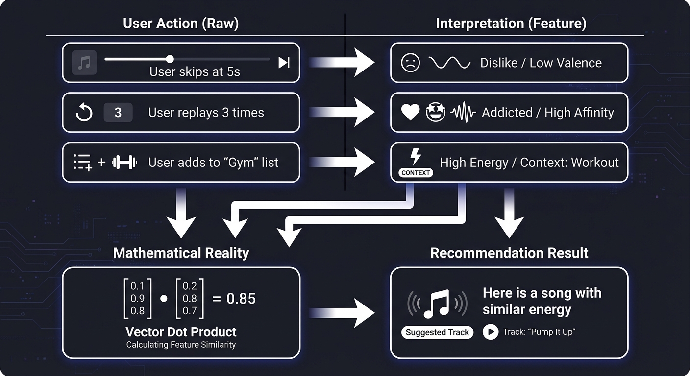
Every “Like,” “Skip,” and “Search” is a signal. Learning to build these engines is learning how to translate human emotion into high-dimensional vectors.
The Recommendation Hierarchy: From Signals to Insights
┌─────────────────────────────────────────────────────────────────┐
│                     THE DISCOVERY STACK                         │
│  ┌──────────────┐                                               │
│  │ Reinforcement│  ← Long-term satisfaction (Bandits, RL)       │
│  └──────┬───────┘                                               │
│         │                                                       │
│  ┌──────┴───────┐                                               │
│  │ Re-ranking   │  ← Diversity, Novelty, Fairness filters       │
│  └──────┬───────┘                                               │
│         │                                                       │
│  ┌──────┴───────┐                                               │
│  │ Candidate Gen│  ← Filtering 100M tracks to 1,000 (SVD, NCF)   │
│  └──────┬───────┘                                               │
│         │                                                       │
│  ┌──────┴───────┐                                               │
│  │ Feature Eng  │  ← MFCCs, Lyrics (BERT), Interaction Matrix   │
│  └──────┬───────┘                                               │
└─────────┼───────────────────────────────────────────────────────┘
          │
┌─────────┴───────────────────────────────────────────────────────┐
│     DATA LAKE   ← Billions of rows of play history & audio files│
└─────────────────────────────────────────────────────────────────┘
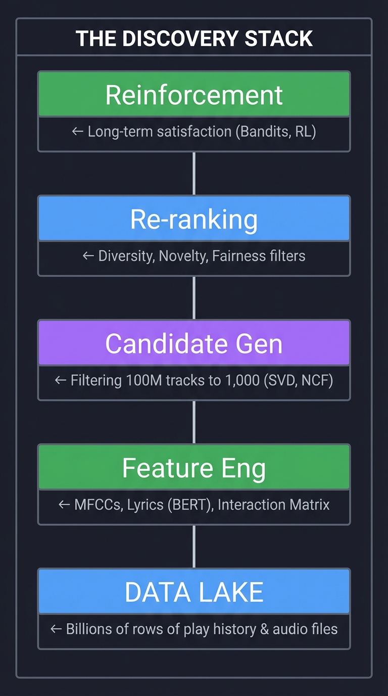
When you build a recommender, you’re not just “predicting a rating”—you’re managing this entire stack. Understanding this is why engineers at Spotify, Apple, and YouTube can keep users engaged for hours.
Core Concept Analysis
1. The Interaction Matrix: Representing Taste
At the heart of Collaborative Filtering is the User-Item matrix. It’s a massive, mostly empty grid of who listened to what.
            Song 1    Song 2    Song 3    Song 4
          (Beatles)  (Metallica) (Jazz)  (EDM)
User A      [ 5 ]      [ 0 ]     [ 1 ]     [ 0 ]
User B      [ 4 ]      [ 1 ]     [ 0 ]     [ 0 ]
User C      [ 0 ]      [ 5 ]     [ 0 ]     [ 4 ]
User D      [ 1 ]      [ 0 ]     [ 5 ]     [ 0 ]
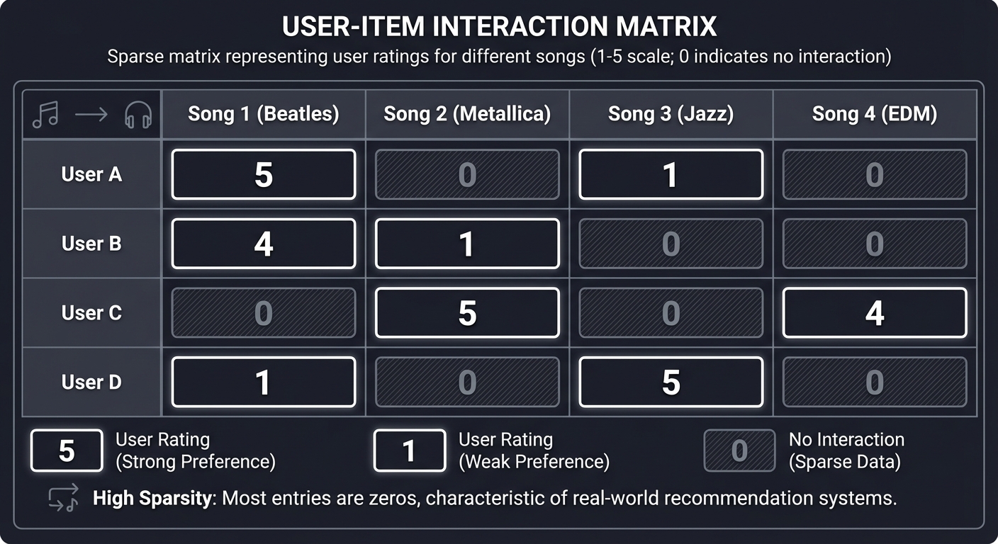
The Sparsity Problem: In a real system (100M users x 10M songs), 99.99% of these cells are 0. Your job is to fill in the blanks. If User A likes Beatles and User B likes Beatles, maybe User A will like Metallica (User B’s other favorite)?
2. Content-Based DNA: Extracting the “Vibe”
If you don’t know who a user is (Cold Start), you look at the song. We turn audio into a “Feature Vector”:
Song: "Midnight City"
┌─────────────────┬───────────┐
│ Feature         │ Value     │
├─────────────────┼───────────┤
│ BPM             │ 105       │
│ Valence (Mood)  │ 0.82      │
│ Acousticness    │ 0.05      │
│ Energy          │ 0.91      │
└─────────────────┴───────────┘
      ↓
Vector: [105, 0.82, 0.05, 0.91]
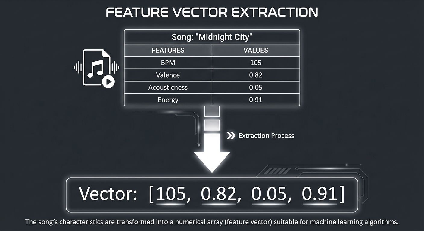
By calculating the Cosine Similarity between vectors, you find songs that “sound” similar regardless of what anyone else thinks.
3. Latent Factors: The Hidden Dimensions of Music
Sometimes, the most important features aren’t visible. Matrix Factorization decomposes the giant matrix into smaller “User Embeddings” and “Item Embeddings”.
User A (Embed)  x  Song X (Embed)  =  Predicted Interest
[0.8, -0.2, 0.5] • [0.9, -0.1, 0.4] =  0.94 (Match!)
Each dimension might represent an abstract concept the machine learned:
- Dimension 1: “Acoustic vs. Electronic”
- Dimension 2: “Sad vs. Happy”
- Dimension 3: “Complexity of Harmony”
4. Hybrid Systems: The Industry Standard
Why choose? Modern systems use Hybrids.
- Candidate Generation: Use CF (SVD/NCF) to grab 1000 potential tracks.
- Scoring: Use Content-Based features + Context (Time of day, Device) to rank those 1000.
- Re-ranking: Apply diversity filters so you don’t show the same artist 10 times.
5. Graph Perspectives: Taste as a Network
Standard Matrix Factorization looks at direct interactions. Graph Neural Networks (GNNs) look at the “hops” between nodes.
(User A) ─── [Song 1] ─── (User B) ─── [Song 2]
Even if User A has never heard Song 2, they are connected via User B and Song 1. This “Collaborative Signal Propagation” is the secret to discovering niche artists in the “Long Tail.”
6. The Exploitation-Exploration Tradeoff
A recommender that only gives you what you already like becomes a “Filter Bubble.” Reinforcement Learning (Multi-Armed Bandits) treats recommendations as experiments:
- Exploitation: Give them more Beatles (High confidence of reward).
- Exploration: Give them an unknown Jazz track (Taking a risk to learn more about their boundaries).
Tools for Understanding Recommendation
1. Pandas & NumPy: The Bedrock
The tools for manipulating the Interaction Matrix.
pivot_table = df.pivot(index='user_id', columns='song_id', values='rating').fillna(0)
2. Scikit-Learn: The Geometry
For calculating distances and similarities.
from sklearn.metrics.pairwise import cosine_similarity
sim = cosine_similarity(song_vectors)
3. Librosa: The “Ears”
For Digital Signal Processing (DSP) of raw audio files.
y, sr = librosa.load('song.mp3')
mfccs = librosa.feature.mfcc(y=y, sr=sr)
4. PyTorch / TensorFlow: The Brain
For deep learning models like Neural Collaborative Filtering (NCF) or Graph Neural Networks (GNNs).
Concept Summary Table
| Concept Cluster | What You Need to Internalize |
|---|---|
| Interaction Matrix | A sparse representation of who listened to what. The primary input for CF. |
| Implicit Feedback | Actions like skips or repeats that signal preference without an explicit “rating.” |
| Similarity Metrics | Cosine vs. Euclidean vs. Jaccard. Choosing the right “ruler” for your data. |
| Matrix Factorization | Decomposing a big sparse matrix into dense “Latent Factor” vectors. |
| Cold Start | The challenge of recommending for new users (no history) or new items (no plays). |
| Embeddings | Dense numerical representations where “similar” things are mathematically “close.” |
| Evaluation Metrics | Precision@K, NDCG, and Hit Rate. How to prove your model actually works. |
| Diversity & Novelty | Balancing “more of what you like” with “something you didn’t know you liked.” |
Deep Dive Reading by Concept
This section maps each concept from above to specific book chapters for deeper understanding. Read these before or alongside the projects to build strong mental models.
Recommendation Fundamentals
| Concept | Book & Chapter |
|---|---|
| Basics of RecSys | Practical Recommender Systems by Kim Falk — Ch. 1: “Introduction to Recommender Systems” |
| User Behavior | Practical Recommender Systems by Kim Falk — Ch. 2: “Collecting and Understanding User Behavior” |
| Content-Based Filtering | Recommender Systems: The Textbook by Charu C. Aggarwal — Ch. 4: “Content-Based Recommender Systems” |
| Collaborative Filtering | Recommender Systems: The Textbook by Charu C. Aggarwal — Ch. 2: “Neighborhood-Based Collaborative Filtering” |
Advanced Modeling & Engineering
| Concept | Book & Chapter |
|---|---|
| Matrix Factorization | Recommender Systems Handbook by Ricci et al. — Part II, Ch. 5: “Matrix Factorization” |
| Deep Learning Recs | Deep Learning for Recommender Systems by Li et al. — Ch. 2-3 (NCF Foundations) |
| Graph Neural Networks | Graph Representation Learning by William L. Hamilton — Ch. 5: “Graph Neural Networks” |
| System Architecture | Designing Data-Intensive Applications by Martin Kleppmann — Ch. 11: “Stream Processing” |
| Active Learning (Bandits) | Reinforcement Learning: An Introduction by Sutton & Barto — Ch. 2: “Multi-Armed Bandits” |
Essential Reading Order
- Foundation (Week 1):
- Practical Recommender Systems Ch. 1-2 (Concepts & Data)
- Practical Recommender Systems Ch. 3 (Content-Based)
- The Collaborative Era (Week 2):
- Practical Recommender Systems Ch. 4 (Collaborative Filtering)
- Recommender Systems: The Textbook Ch. 2 (Implicit Feedback)
- Production Scale (Week 3+):
- Designing Data-Intensive Applications Ch. 3 (Storage/Retrieval)
- Recommender Systems Handbook Part II, Ch. 5 (Math of Latent Factors)
Project List
Projects are ordered from fundamental similarity logic to advanced production architectures.
Project 1: “Simple Content-Based Music Recommender” — Feature Engineering
| Attribute | Details |
|---|---|
| File | MUSIC_RECOMMENDATION_ENGINE_LEARNING_PROJECTS.md |
| Main Programming Language | Python |
| Alternative Programming Languages | JavaScript, R |
| Coolness Level | Level 2: Practical but Forgettable |
| Business Potential | 1. The “Resume Gold” |
| Difficulty | Level 1: Beginner |
| Knowledge Area | Content-Based Filtering, Feature Engineering |
| Software or Tool | Pandas, Scikit-learn |
| Main Book | “Practical Recommender Systems” by Kim Falk |
What you’ll build: A system that suggests songs based on matching characteristics (genre, artist, tempo) of songs a user already likes.
Why it teaches music recommendation: It forces you to digitize the “DNA” of a song. You’ll learn how to represent categories (like Genre) as numbers and how to calculate “distance” in high-dimensional space.
Core challenges you’ll face:
- One-Hot Encoding → mapping categorical data to vectors.
- Normalizing Tempo → ensuring BPM (120) doesn’t drown out Genre (0 or 1).
- The Filter Bubble → realizing your system only recommends “more of the same.”
Real World Outcome
You’ll have a script that takes a “Seed Song” and finds the 5 most similar tracks in a CSV catalog.
Example Output:
$ python content_recommender.py --seed "Uptown Funk"
Seed Song: Uptown Funk (Genre: Funk, BPM: 115)

Top Recommendations:
1. Treasure (Bruno Mars) - Match: 98% (Same Artist, Same Genre)
2. Get Lucky (Daft Punk) - Match: 85% (Same Genre, Close BPM)
3. Happy (Pharrell) - Match: 82% (High Energy, Funk elements)

# You are seeing how metadata alone can create a surprisingly coherent 'vibe'!
The Core Question You’re Answering
“If I only know about the items, and nothing about other users, how can I find a ‘sibling’ for this song?”
Before coding, realize that “similarity” is subjective. To a computer, similarity is just two vectors pointing in the same direction in a many-dimensional room.
Concepts You Must Understand First
Stop and research these before coding:
- Feature Vectors & Embeddings
- How do you turn a “Genre” (string) into a “Feature” (number)?
- Why do we use One-Hot Encoding?
- Book Reference: “Practical Recommender Systems” Ch. 3
- Distance vs. Similarity
- What is the difference between Euclidean Distance and Cosine Similarity?
- Why is Cosine Similarity the “gold standard” for recommendation?
- Book Reference: “Recommender Systems: The Textbook” Ch. 4
- Normalization (Feature Scaling)
- If Tempo is 120 and Valence is 0.5, why will Tempo dominate the math?
- How does Min-Max Scaling solve this?
Questions to Guide Your Design
Before implementing, think through these:
- Defining the ‘DNA’
- Which features matter most? Tempo? Key? Danceability?
- How do you handle missing data (e.g., a song with no genre)?
- The Similarity Matrix
- Should you calculate similarity for every song pair every time?
- How do you store the similarity scores for fast lookup?
- User Profile Creation
- If a user likes 3 songs, how do you create a single “User Vector” that represents their taste? (Average? Weighted average?)
Thinking Exercise
Trace the Similarity By Hand
Imagine 3 songs:
- Song A: BPM=120, Genre=Rock (1)
- Song B: BPM=125, Genre=Rock (1)
- Song C: BPM=120, Genre=Jazz (0)
Questions while tracing:
- Which is more similar to A: B or C?
- If you change the BPM of B to 180, is it still “similar” to A?
- How much does the Genre column “weight” the result compared to BPM?
The Interview Questions They’ll Ask
Prepare to answer these:
- “What are the limitations of Content-Based Filtering?” (Answer: The Filter Bubble / Overspecialization)
- “How do you handle categorical features like ‘Artist’ when there are thousands of them?”
- “Explain the ‘Cold Start’ problem for items in Content-Based systems. (Trick question: Content-based systems solve the item cold start!)”
Hints in Layers
Hint 1: Start with a CSV
Don’t build a database yet. Use a CSV with columns like title, artist, genre, tempo.
Hint 2: One-Hot Encoding
Use pandas.get_dummies() to transform your genre column into multiple binary columns.
Hint 3: Calculating Similarity
Use sklearn.metrics.pairwise.cosine_similarity. It takes a matrix and returns a matrix of similarity scores.
Hint 4: Ranking
Use argsort() to find the indices of the highest similarity scores, excluding the seed song itself.
Books That Will Help
| Topic | Book | Chapter |
|---|---|---|
| Content-Based Logic | “Practical Recommender Systems” | Ch. 3 |
| Math of Similarity | “Recommender Systems: The Textbook” | Ch. 4 |
| Feature Engineering | “Building Recommender Systems with ML” | Ch. 2 |
Project 2: “User-Based Collaborative Filtering” — UCF
| Attribute | Details |
|---|---|
| File | MUSIC_RECOMMENDATION_ENGINE_LEARNING_PROJECTS.md |
| Main Programming Language | Python |
| Alternative Programming Languages | Scala, Java |
| Coolness Level | Level 3: Genuinely Clever |
| Business Potential | 1. The “Resume Gold” |
| Difficulty | Level 2: Intermediate |
| Knowledge Area | Collaborative Filtering, User Similarity |
| Software or Tool | NumPy, Pandas |
| Main Book | “Practical Recommender Systems” by Kim Falk |
What you’ll build: A system that finds users with similar tastes and recommends songs they liked that the target user hasn’t heard yet.
Why it teaches music recommendation: This is the leap from “item matching” to “social matching.” You’ll grapple with the User-Item Matrix and the reality of Sparsity (most users only listen to 0.001% of all songs).
Core challenges you’ll face:
- Handling Sparsity → What to do with the “holes” in your data.
- Cold Start (Users) → Realizing you can’t recommend anything to a user who hasn’t liked a song yet.
- The “Mean Centering” Problem → Handling users who “like” everything vs users who are very stingy with likes.
Real World Outcome
You’ll have a Python script that generates a “Discovery” list for a specific User ID based on the behavior of their “musical soulmates.”
Example Output:
$ python user_cf.py --user_id 405
User 405 likes: [Classic Rock, Blues]
Found 10 Similar Users (Soulmates).

User 405 might also like:
1. The Thrill is Gone (B.B. King) - Liked by 8 soulmates.
2. Crossroads (Cream) - Liked by 5 soulmates.
3. Voodoo Child (Jimi Hendrix) - Liked by 4 soulmates.

# You've just automated "word of mouth" discovery!
The Core Question You’re Answering
“If I know what you like, and I know what people like you like, how can I use their history to predict your future?”
This project forces you to think about the “Wisdom of the Crowd.” You’ll learn that the strongest signal for recommendation isn’t the item’s features, but the behavior of similar humans.
Concepts You Must Understand First
Stop and research these before coding:
- The User-Item Matrix
- What is an “interaction” (row=user, col=song)?
- Why do we call it a “Pivot Table”?
- Book Reference: “Practical Recommender Systems” Ch. 4
- The Curse of Sparsity
- Why do 99% of the cells in your matrix have zeros?
- How does sparsity break Euclidean distance?
- Book Reference: “Recommender Systems: The Textbook” Ch. 10
- K-Nearest Neighbors (KNN)
- How do you define a “neighbor”?
- What is the tradeoff between a small K (few neighbors) and a large K?
Questions to Guide Your Design
Before implementing, think through these:
- Similarity Logic
- If User A liked 5 songs and User B liked 100 songs, but they have 2 songs in common, are they “similar”?
- Scoring Recommendations
- Should a song liked by your #1 most similar neighbor count more than a song liked by your #10 neighbor?
- Handling Popularity
- How do you stop your system from just recommending the top 5 global hits to everyone?
Thinking Exercise
Tracing the Matrix
Imagine a 3x3 matrix:
- User 1: [1, 0, 1] (Likes S1, S3)
- User 2: [1, 1, 0] (Likes S1, S2)
- User 3: [0, 1, 1] (Likes S2, S3)
Questions:
- Which user is most similar to User 1? (Answer: User 2 and User 3 are equally similar - 1 song in common).
- If User 1 hasn’t heard Song 2, but User 2 (his neighbor) has, should you recommend it?
- What happens if a new user (User 4) joins with [0, 0, 0]? Who is their neighbor?
The Interview Questions They’ll Ask
Prepare to answer these:
- “What is the difference between User-Based and Item-Based CF?”
- “How do you handle the ‘Cold Start’ problem for a new user in CF?”
- “Why does Cosine Similarity work better than Euclidean distance for sparse data?”
- “Explain ‘Shilling Attacks’ - how can a user manipulate your UCF system?”
Hints in Layers
Hint 1: The Matrix Pivot
Start by using df.pivot(index='user_id', columns='song_id', values='rating'). This is your interaction matrix.
Hint 2: The Similarity Calculation
Use sklearn.metrics.pairwise.cosine_similarity(matrix). This will give you a User-User similarity matrix.
Hint 3: Finding Neighbors For User X, sort their row in the similarity matrix to find the top K users.
Hint 4: Aggregating Votes Look at the songs those K neighbors liked that User X has NOT seen. Sum their similarity scores to get a final recommendation score for each song.
Books That Will Help
| Topic | Book | Chapter |
|---|---|---|
| CF Foundations | “Practical Recommender Systems” | Ch. 4 |
| Neighborhood Models | “Recommender Systems: The Textbook” | Ch. 2 |
| Matrix Operations | “Python for Data Analysis” | Ch. 5 |
Project 3: “Item-Based Collaborative Filtering” — ICF
| Attribute | Details |
|---|---|
| File | MUSIC_RECOMMENDATION_ENGINE_LEARNING_PROJECTS.md |
| Main Programming Language | Python |
| Alternative Programming Languages | Java, R |
| Coolness Level | Level 3: Genuinely Clever |
| Business Potential | 3. The “Service & Support” Model |
| Difficulty | Level 2: Intermediate |
| Knowledge Area | Item-Item Similarity, Scalability |
| Software or Tool | Scikit-learn, Pandas |
| Main Book | “Recommender Systems Handbook” Part I, Ch. 2 |
What you’ll build: Instead of finding similar users, you’ll find similar items based on co-occurrence (e.g., “People who liked X also liked Y”).
Why it teaches music recommendation: In the real world, catalogs (songs) change slower than users. Item-item similarity is more stable and scalable than user-user similarity. You’ll learn why Amazon and Netflix historically preferred this.
Core challenges you’ll face:
- Transposing the Matrix → Re-orienting your view from “User rows” to “Song rows.”
- Popularity Bias → Realizing everyone listens to “Shape of You,” making it “similar” to every other song by accident.
Real World Outcome
You’ll have a script that, given a song the user is currently listening to, finds “Related Tracks” based on the patterns of millions of other users.
Example Output:
$ python item_cf.py --current_track "Bohemian Rhapsody"
Track: Bohemian Rhapsody (Queen)

People who liked this also liked:
1. Don't Stop Me Now (Queen) - Similarity: 0.92
2. Rocket Man (Elton John) - Similarity: 0.85
3. Stairway to Heaven (Led Zeppelin) - Similarity: 0.81

# You are seeing how the item itself can be a portal to other similar content!
The Core Question You’re Answering
“Can I recommend a song based on the ‘company it keeps’ in other people’s libraries?”
You’ll learn that items have “personalities” defined by the groups of people who consume them.
Concepts You Must Understand First
Stop and research these before coding:
- Item Similarity Matrix
- Why is the similarity matrix N x N (songs x songs) instead of U x U (users x users)?
- Book Reference: “Recommender Systems Handbook” Part I, Ch. 2
- Persistence & Precomputation
- Why is it easier to save item similarities than user similarities?
- How often do you need to update an Item-Item matrix?
- Adjusted Cosine Similarity
- Why do we subtract the user’s average rating from each rating before calculating similarity?
- Book Reference: “Recommender Systems: The Textbook” Ch. 2.3
Questions to Guide Your Design
Before implementing, think through these:
- Catalog Scale
- If you have 1 million songs, your similarity matrix has 1 trillion cells (1M x 1M). How do you handle this? (Sparse matrices!)
- Popularity Penalization
- If a song is in 90% of all playlists, it will appear similar to everything. How do you penalize this “global popular” signal?
- Filtering by Correlation
- Should you only look at items with a minimum number of overlapping users (e.g., at least 50 people must have liked both songs)?
Thinking Exercise
The Amazon Strategy
Trace this scenario:
- 100 million users.
- 1 million songs.
- A user’s taste changes every day.
- A song’s similarity to other songs (based on history) changes slowly.
Questions:
- Why is it cheaper to calculate “Similar Items” once a day than to find “Similar Users” every time a user logs in?
- What happens to your Item-Item matrix when a brand new song is uploaded? (Cold Start!)
The Interview Questions They’ll Ask
Prepare to answer these:
- “Why is Item-Based CF generally more stable than User-Based CF?”
- “Explain the ‘Slop One’ algorithm - why is it a popular alternative for Item-Based CF?”
- “How do you handle ‘Popularity Bias’ where the top hit is similar to everything?”
Hints in Layers
Hint 1: Transpose the Data Your matrix should now have songs as rows and users as columns.
Hint 2: Sparse Matrix Usage
Use scipy.sparse.csr_matrix to save memory. 99% of your data is likely zeros.
Hint 3: Calculating Item Similarity
Use cosine_similarity(matrix_transposed).
Hint 4: Serving Recommendations To recommend for User A: Find the songs they liked, look up those songs’ most similar siblings in your matrix, and aggregate the scores.
Books That Will Help
| Topic | Book | Chapter |
|---|---|---|
| Item-Item Models | “Recommender Systems Handbook” | Part I, Ch. 2 |
| Sparse Data Handling | “Python for Data Analysis” | Ch. 12 |
| Scalable Similarity | “Mining of Massive Datasets” | Ch. 3 |
Project 4: “Hybrid Music Recommender” — Simple Blending
| Attribute | Details |
|---|---|
| File | MUSIC_RECOMMENDATION_ENGINE_LEARNING_PROJECTS.md |
| Main Programming Language | Python |
| Alternative Programming Languages | Java, Go |
| Coolness Level | Level 3: Genuinely Clever |
| Business Potential | 2. The “Micro-SaaS / Pro Tool” |
| Difficulty | Level 3: Advanced |
| Knowledge Area | Hybrid Systems, Cold Start |
| Software or Tool | Pandas, NumPy |
| Main Book | “Practical Recommender Systems” Ch. 5 |
What you’ll build: A system that merges the scores from your Content-Based model and your Collaborative model to provide a single ranked list.
Why it teaches music recommendation: This project solves the “Cold Start” problem. When a new user joins (no history for CF), you fall back to Content-Based features. As they listen more, you shift the weights toward Collaborative data.
Core challenges you’ll face:
- Score Normalization → How to combine a “0.9 similarity score” with a “4.5 predicted rating.”
- Weight Tuning → Finding the right balance between “Discovery” (CF) and “Consistency” (Content).
Real World Outcome
A recommender that works for EVERYONE—even users who just signed up 1 minute ago.
Example Output:
$ python hybrid_recommender.py --user_id NEW_USER --seed_genre "Jazz"
[Cold Start Logic Triggered: Using Content-Based fallback]
1. Kind of Blue (Miles Davis) - Score: 0.95 (Based on Genre Match)

$ python hybrid_recommender.py --user_id OLD_USER
[Collaborative Logic Triggered: 70% CF, 30% Content]
1. New Discovery (Artist X) - Score: 0.88 (Strong Social Signal)
2. Similar Sounding (Artist Y) - Score: 0.72 (Content Signal)

# You are seeing a system that gracefully adapts to the volume of data available!
The Core Question You’re Answering
“How do I build a system that never says ‘I don’t know what you like’?”
Concepts You Must Understand First
Stop and research these before coding:
- Hybrid Architectures
- What is the difference between “Weighted,” “Switching,” and “Feature Augmentation” hybrids?
- Book Reference: “Practical Recommender Systems” Ch. 5
- Score Normalization
- How do you scale outputs from two different algorithms so they can be added together? (e.g., Min-Max or Z-Score)
- The Cold Start Decay
- How do you mathematically “fade in” the Collaborative signal as more data becomes available?
Questions to Guide Your Design
Before implementing, think through these:
- The ‘Switching’ Point
- How many songs must a user like before you trust the Collaborative model?
- Feature Weights
- Should “Genre” count more than “Tempo” in the Content side?
- Should “User Soulmate” count more than “Item Co-occurrence” in the Collaborative side?
- Handling Disagreement
- What if the Content model loves a song but the CF model thinks it’s a 1-star match? How do you resolve the conflict?
Thinking Exercise
The Balance of Power
Imagine a user who has liked 1 song: “Thriller” by Michael Jackson.
- Content model suggests: “Beat It” (Same Artist, Same Genre).
- CF model suggests: “1999” by Prince (People who liked Thriller also liked Prince).
Questions:
- If you weight them 50/50, which song wins?
- If the user likes 10 more Michael Jackson songs, should the CF weight increase or decrease?
The Interview Questions They’ll Ask
Prepare to answer these:
- “Why are hybrid systems the standard in production (Netflix, Spotify, Amazon)?”
- “How would you design a ‘Cascading Hybrid’ system?”
- “Explain how a Hybrid system solves the Item Cold Start problem.”
Hints in Layers
Hint 1: Run them in Parallel Run your Project 1 script and Project 2 script on the same dataset. Get two sets of scores.
Hint 2: Min-Max Scaling
Scale both sets of scores to the [0, 1] range.
normalized = (x - min) / (max - min)
Hint 3: The Weighted Average
final_score = (alpha * CF_score) + ((1 - alpha) * Content_score)
Start with alpha = 0.5.
Hint 4: Adaptive Alpha
Try making alpha = min(1.0, num_user_ratings / 20). This means after 20 ratings, you are 100% CF.
Books That Will Help
| Topic | Book | Chapter |
|---|---|---|
| Hybrid Models | “Practical Recommender Systems” | Ch. 5 |
| Normalization | “Hands-On ML with Scikit-Learn” | Ch. 2 |
Project 5: “Music Genre Classifier” — Digital Signal Processing
| Attribute | Details |
|---|---|
| File | MUSIC_RECOMMENDATION_ENGINE_LEARNING_PROJECTS.md |
| Main Programming Language | Python |
| Alternative Programming Languages | C++ (for real-time), MATLAB |
| Coolness Level | Level 4: Hardcore Tech Flex |
| Business Potential | 4. The “Open Core” Infrastructure |
| Difficulty | Level 3: Advanced |
| Knowledge Area | Audio Processing, Machine Learning |
| Software or Tool | Librosa, Scikit-learn |
| Main Book | “Deep Learning for Audio Signal Processing” Ch. 2 |
What you’ll build: A model that “listens” to raw .wav files and classifies them into Genres (Rock, Jazz, Pop) using features like MFCCs.
Why it teaches music recommendation: You move from using “human tags” to “automatic features.” This is how Spotify handles new uploads that have no metadata yet.
Core challenges you’ll face:
- Spectrogram Generation → Visualizing sound.
- MFCC Extraction → Capturing the “texture” of human voice vs electric guitar.
- Temporal Averaging → Turning a 3-minute song into a single fixed-size feature vector.
Real World Outcome
You’ll have a model that can take a raw MP3 file and correctly label its genre based on its acoustic properties.
Example Output:
$ python classify_audio.py --file "new_track.mp3"
Analyzing Spectrogram...
Extracting MFCCs (Mel-frequency cepstral coefficients)...
Computing Spectral Centroid...

Prediction: Jazz (92% confidence)
Acoustic Profile:
- Tempo: 78 BPM (Slow)
- Harmonic Complexity: High
- Percussiveness: Low

# You are seeing how a machine 'hears' the difference between instruments and rhythms!
The Core Question You’re Answering
“How can a machine ‘hear’ the difference between a violin and a distorted guitar?”
You’ll discover that sound is just a wave, and machine learning can find patterns in the frequencies that human ears intuitively recognize.
Concepts You Must Understand First
Stop and research these before coding:
- Digital Signal Processing (DSP) Basics
- What is a Sampling Rate (e.g., 44.1kHz)?
- What is the Nyquist Theorem?
- Book Reference: “Deep Learning for Audio Signal Processing” Ch. 2
- Fast Fourier Transform (FFT)
- How do we turn time-series sound (amplitude over time) into frequency “buckets”?
- What is a Spectrogram?
- MFCCs (Mel-frequency cepstral coefficients)
- Why do we use the “Mel” scale? (Hint: It mimics how humans hear pitch).
- Why are MFCCs the “gold standard” for audio classification?
Questions to Guide Your Design
Before implementing, think through these:
- Windowing
- Should you analyze the whole 3-minute song at once, or in small chunks (e.g., 20ms windows)?
- Feature Fusion
- Can you combine MFCCs with other features like “Zero Crossing Rate” or “Chroma Features”?
- Data Augmentation
- How do you make your model robust to noise or different recording qualities?
Thinking Exercise
The Spectrogram Visualization
Look at a spectrogram of a Drum & Bass track vs. a solo Piano piece.
- Question: Where do you expect to see the most energy (brightness) in the D&B track? (Answer: Low frequency/Bass).
- Question: How does the “texture” of the image change for the Piano piece compared to a heavily distorted Rock guitar?
The Interview Questions They’ll Ask
Prepare to answer these:
- “Explain the difference between a Spectrogram and a Mel-Spectrogram.”
- “Why are MFCCs better for speech/music recognition than raw audio waveforms?”
- “How do you handle audio files of different lengths when feeding them into a neural network?”
Hints in Layers
Hint 1: Librosa is your best friend
Use librosa.load() and librosa.feature.mfcc().
Hint 2: Visualization
Use librosa.display.specshow() with matplotlib to see the audio before you classify it.
Hint 3: Data Source Use the GTZAN Genre Collection dataset. It’s the “MNIST” of audio genre classification.
Hint 4: Classification Start with a simple Random Forest or SVM classifier before jumping into Deep Learning (CNNs).
Books That Will Help
| Topic | Book | Chapter |
|---|---|---|
| Audio DSP | “Deep Learning for Audio Signal Processing” | Ch. 2-3 |
| Music Information Retrieval | “An Introduction to Audio Content Analysis” | Ch. 4 |
| Scikit-Learn ML | “Python Machine Learning” | Ch. 3 |
Project 6: “Matrix Factorization Recommender” — SVD/ALS
| Attribute | Details |
|---|---|
| File | MUSIC_RECOMMENDATION_ENGINE_LEARNING_PROJECTS.md |
| Main Programming Language | Python |
| Alternative Programming Languages | Scala (Spark MLlib), Java |
| Coolness Level | Level 4: Hardcore Tech Flex |
| Business Potential | 1. The “Resume Gold” |
| Difficulty | Level 4: Expert |
| Knowledge Area | Latent Factor Modeling, Optimization |
| Software or Tool | Surprise Library, NumPy |
| Main Book | “Recommender Systems Handbook” Part II, Ch. 5 |
What you’ll build: A system that factorizes the giant user-item matrix into dense embedding vectors.
Why it teaches music recommendation: This is the “Netflix Prize” technique. You’ll learn that you don’t need to manually define features; the math finds “Hidden Dimensions” (e.g., a dimension that automatically correlates with ‘acousticness’) purely from interaction patterns.
Core challenges you’ll face:
- Implicit Feedback → Handling the fact that a “non-play” doesn’t necessarily mean a “dislike.”
- Overfitting → Preventing the model from just memorizing the training data.
Real World Outcome
A system that can predict the exact rating a user would give to a song they’ve never heard, using “Latent Factors.”
Example Output:
$ python matrix_fact.py --user 10 --song 500
User 10 Predicted Rating for 'Stairway to Heaven': 4.8 / 5.0

Analysis of Latent Factors for User 10:
- Affinity for Factor #1 (Acoustic vs Electronic): High (Acoustic)
- Affinity for Factor #3 (Complexity): High (Prog Rock vibes)
- Affinity for Factor #7 (Era): 70s-80s Bias

# You are seeing the 'hidden' logic of human taste being mathematically extracted!
The Core Question You’re Answering
“If I represent every user as 50 numbers and every song as 50 numbers, can the dot product between them reveal the secrets of human taste?”
Concepts You Must Understand First
Stop and research these before coding:
- Matrix Decomposition
- What is SVD (Singular Value Decomposition)?
- How does
R ≈ U x Vwork, where R is the interaction matrix? - Book Reference: “Recommender Systems Handbook” Part II, Ch. 5
- Latent Factors
- What does it mean for a feature to be “Latent”?
- Why do we choose a specific number of factors (e.g., 50 or 100)?
- Alternating Least Squares (ALS)
- Why is ALS better for large-scale production than standard SVD?
- Book Reference: “Practical Recommender Systems” Ch. 8
Questions to Guide Your Design
Before implementing, think through these:
- Regularization
- How do you prevent your model from over-fitting to the few ratings a user has provided?
- Cold Start Strategy
- If a new song has NO interactions, how do you assign its latent factors? (Hint: You can’t with MF alone!)
- Hyperparameter Tuning
- How do you choose the number of factors (Rank)?
- What happens if the rank is too low (Underfitting) or too high (Overfitting)?
Thinking Exercise
Visualizing Latent Dimensions
Imagine a 2-factor model:
- Factor 1: Energy (High to Low)
- Factor 2: Organic (Acoustic to Synthetic)
Questions:
- Where would “Metallica” sit in this 2D space?
- Where would “Mozart” sit?
- If a User vector points toward [High Energy, Synthetic], what songs should you recommend?
The Interview Questions They’ll Ask
Prepare to answer these:
- “What is the difference between explicit and implicit matrix factorization?”
- “Explain the ‘Cold Start’ problem in the context of Matrix Factorization.”
- “How does the dot product relate to Cosine Similarity in a normalized latent space?”
- “Why did the Netflix Prize winner use Matrix Factorization?”
Hints in Layers
Hint 1: Use the Surprise Library
Use surprise.SVD for a quick and robust implementation.
Hint 2: Cross-Validation
Use surprise.model_selection.cross_validate to measure your RMSE (Root Mean Squared Error).
Hint 3: Interpretation Try to visualize the items with the highest and lowest values for a specific latent factor. Do they share a common genre or vibe?
Hint 4: Large Scale
If you want to build this for millions of users, look into implicit (ALS for implicit feedback) or Spark MLlib.
Books That Will Help
| Topic | Book | Chapter |
|---|---|---|
| Matrix Math | “Linear Algebra Done Right” | Ch. 7 |
| MF for Recs | “Recommender Systems Handbook” | Part II, Ch. 5 |
| Practical SVD | “Practical Recommender Systems” | Ch. 8 |
Project 7: “Neural Collaborative Filtering” — NCF
| Attribute | Details |
|---|---|
| File | MUSIC_RECOMMENDATION_ENGINE_LEARNING_PROJECTS.md |
| Main Programming Language | Python |
| Alternative Programming Languages | TensorFlow.js, C++ (libtorch) |
| Coolness Level | Level 5: Pure Magic (Super Cool) |
| Business Potential | 5. The “Industry Disruptor” |
| Difficulty | Level 5: Master |
| Knowledge Area | Deep Learning, Neural Networks |
| Software or Tool | TensorFlow/Keras, PyTorch |
| Main Book | “Deep Learning for Recommender Systems” Ch. 3 |
What you’ll build: A deep learning model that learns complex, non-linear interactions between users and items using embeddings and Multi-Layer Perceptrons (MLPs).
Why it teaches music recommendation: It moves beyond the linear math of Matrix Factorization. You’ll learn how to feed IDs into embedding layers and let the network learn the “logic” of taste.
Core challenges you’ll face:
- Negative Sampling → Since you only see “what users liked,” you have to generate “fake dislikes” to train the network.
- Embedding Dimensionality → Choosing how many numbers represent a user (32? 128? 512?).
Real World Outcome
A deep neural network that recommends music with significantly higher accuracy than linear matrix factorization, capable of identifying subtle “non-linear” taste patterns.
Example Output:
$ python ncf_train.py --epochs 10
Epoch 10: Loss 0.12, Validation Hit@10: 0.85

$ python ncf_predict.py --user 5
Top Neural Recommendations:
1. Starboy (The Weeknd) - Confidence Score: 0.99
2. Blinding Lights (The Weeknd) - Confidence Score: 0.97
3. Save Your Tears (The Weeknd) - Confidence Score: 0.94

# You are seeing a Deep Learning model that has identified a 'Genre/Artist Cluster' with high precision!
The Core Question You’re Answering
“Why limit our taste model to simple dot products? Can a Deep Neural Network find non-linear connections in our musical journey?”
Concepts You Must Understand First
Stop and research these before coding:
- Embedding Layers
- How do you turn a discrete ID (User 523) into a dense vector of weights?
- What happens to these weights during backpropagation?
- Book Reference: “Deep Learning for Recommender Systems” Ch. 2
- GMF vs MLP
- What is General Matrix Factorization (GMF) in a neural context?
- Why do we combine it with a Multi-Layer Perceptron (MLP)?
- Book Reference: “Deep Learning for Recommender Systems” Ch. 3 (NeuRec Architecture)
- Negative Sampling
- If your dataset only has “Positive” signals (User listened to X), how does the model learn what the user doesn’t like?
- How do you generate high-quality “negative” examples?
Questions to Guide Your Design
Before implementing, think through these:
- The Fusion Layer
- How should you combine the GMF and MLP outputs? (Concatenation? Element-wise product?)
- Loss Functions
- Should you use Binary Cross Entropy (BCE) or Mean Squared Error (MSE)?
- Dropout & Regularization
- How do you prevent a model with 1 million embedding parameters from memorizing your training set?
Thinking Exercise
The Neural Advantage
Imagine two users who both like “Jazz.”
- User A likes “Upbeat Jazz” for running.
- User B likes “Slow Jazz” for reading. Matrix Factorization might just see “Jazz” and recommend the same things.
Question:
- How can a Deep Neural Network with multiple layers (MLP) distinguish between these “sub-contextual” preferences that a simple dot product might miss?
The Interview Questions They’ll Ask
Prepare to answer these:
- “Why use Neural Collaborative Filtering over standard SVD?”
- “Explain the architecture of NeuMF (Neural Matrix Factorization).”
- “How do you handle the ‘Sparsity’ problem in a Neural Network training loop?”
- “What is the purpose of the ‘Activation Function’ (e.g., ReLU) in the MLP branch of NCF?”
Hints in Layers
Hint 1: The Input Pipeline
Your model should take two inputs: user_id and item_id.
Hint 2: Embedding Layers
Use keras.layers.Embedding(num_users, embedding_dim).
Hint 3: The MLP Branch
Start with a architecture like [64, 32, 16] for your hidden layers.
Hint 4: Training
Map your “Listen” events to a target of 1. Randomly sample items the user hasn’t heard and map them to a target of 0.
Books That Will Help
| Topic | Book | Chapter |
|---|---|---|
| Neural Recs Foundations | “Deep Learning for Recommender Systems” | Ch. 2-3 |
| Keras/TensorFlow for Recs | “Hands-On Recommendation Systems with Python” | Ch. 11 |
| NCF Original Paper | “Neural Collaborative Filtering” by He et al. | Entire Paper |
Project 8: “Real-time Recommendation API” — MLOps
| Attribute | Details |
|---|---|
| File | MUSIC_RECOMMENDATION_ENGINE_LEARNING_PROJECTS.md |
| Main Programming Language | Python (FastAPI) |
| Alternative Programming Languages | Go, Java (Spring Boot) |
| Coolness Level | Level 3: Genuinely Clever |
| Business Potential | 4. The “Open Core” Infrastructure |
| Difficulty | Level 4: Expert |
| Knowledge Area | Backend Engineering, MLOps |
| Software or Tool | Docker, FastAPI, Redis |
| Main Book | “Designing Data-Intensive Applications” Ch. 3 |
What you’ll build: A production-ready API that serves recommendations in <100ms.
Why it teaches music recommendation: In the real world, nobody waits 10 seconds for a playlist to load. You’ll learn how to pre-compute embeddings and use Redis for fast retrieval.
Core challenges you’ll face:
- Latency → Model inference can be slow; you’ll learn how to cache.
- Dependency Management → Using Docker to ensure your ML model runs on any server.
Real World Outcome
A live, containerized endpoint that responds to JSON requests with low latency, suitable for a real-world app frontend.
Example Output:
$ curl http://localhost:8000/rec/user/10
{
  "user_id": 10,
  "recommendations": [
    {"song_id": "abc-123", "title": "Starlight", "score": 0.98},
    {"song_id": "xyz-789", "title": "Moonlight", "score": 0.92}
  ],
  "latency": "42ms",
  "source": "redis_cache",
  "model_version": "v2.1-ncf"
}

# You are seeing the bridge between a static ML model and a live, scalable product!
The Core Question You’re Answering
“How do I turn a Jupyter Notebook experiment into a service that millions of people can use simultaneously?”
Concepts You Must Understand First
Stop and research these before coding:
- REST API Fundamentals
- What are the differences between GET and POST in an ML context?
- How do you structure JSON responses for a recommender?
- In-Memory Caching (Redis)
- Why is reading from RAM (Redis) faster than calculating with a CPU (inference)?
- What is the “Pre-compute and Cache” pattern?
- Containerization (Docker)
- Why “but it works on my machine” is the enemy of production ML.
- How do you pack a Python environment into an image?
Questions to Guide Your Design
Before implementing, think through these:
- Batch vs Online Inference
- Should you calculate recommendations for all users every night (Batch)?
- Or calculate them only when the user logs in (Online)?
- The 100ms Budget
- If your API takes 500ms, the user will feel a lag. How do you shave off those milliseconds?
- Model Versioning
- How do you deploy a new version of the model without stopping the API? (Blue/Green deployment)
Thinking Exercise
The Scale Challenge
Imagine 1,000 users per second hitting your /rec endpoint.
- Your model takes 50ms to run.
- Your database takes 200ms to fetch user history.
Questions:
- What happens to your server?
- How does adding a Redis layer with pre-computed results solve this?
- What’s the tradeoff? (Answer: Data Freshness).
The Interview Questions They’ll Ask
Prepare to answer these:
- “How do you handle model serving at scale?”
- “Explain the difference between a Feature Store and a standard database.”
- “What is an ‘Approximate Nearest Neighbor’ (ANN) search, and why is it used in large-scale recommenders?”
- “How do you monitor the health of an ML API?”
Hints in Layers
Hint 1: Use FastAPI It’s the fastest Python web framework for ML serving.
Hint 2: The Model Loader
Load your model once when the app starts (using @app.on_event("startup")), NOT inside the request function.
Hint 3: Use Redis for Embeddings
Store your User and Item vectors in Redis. Use a library like Faiss for lightning-fast similarity search if you want to be extra advanced.
Hint 4: Dockerize
Write a simple Dockerfile using python:3.9-slim as the base.
Books That Will Help
| Topic | Book | Chapter |
|---|---|---|
| System Design | “Designing Data-Intensive Applications” | Ch. 1-3 |
| MLOps | “Introducing MLOps” | Ch. 4 |
| FastAPI | “FastAPI Documentation” | Tutorial |
Project 9: “Evaluation Framework” — Offline Metrics
| Attribute | Details |
|---|---|
| File | MUSIC_RECOMMENDATION_ENGINE_LEARNING_PROJECTS.md |
| Main Programming Language | Python |
| Alternative Programming Languages | R, MATLAB |
| Coolness Level | Level 2: Practical but Forgettable |
| Business Potential | 3. The “Service & Support” Model |
| Difficulty | Level 3: Advanced |
| Knowledge Area | Statistics, Data Science |
| Software or Tool | NumPy, Pandas |
| Main Book | “Practical Recommender Systems” Ch. 6 |
What you’ll build: A suite of tools to calculate Precision@K, Recall@K, and NDCG.
Why it teaches music recommendation: “I like the results” is not a scientific measurement. You’ll learn how to objectively prove that Algorithm A is better than Algorithm B.
Core challenges you’ll face:
- Time-Based Splitting → Ensuring you don’t “cheat” by training on the future to predict the past.
- Ranking Metrics → Learning why it’s more important to get the #1 recommendation right than the #50.
Real World Outcome
A comprehensive leaderboard comparing all your previous models using industry-standard statistical benchmarks.
Example Output:
Model Comparison Report:
--------------------------------------------------
Model             | Precision@10 | Recall@10 | NDCG@10
--------------------------------------------------
SVD (Matrix Fact) | 0.12         | 0.05      | 0.22
Neural Coll. Filt | 0.25         | 0.11      | 0.35  <-- WINNER
Content-Based     | 0.08         | 0.03      | 0.15
--------------------------------------------------

Analysis: NCF shows a 40% improvement in ranking quality (NDCG) over traditional SVD.

# You are seeing how data science provides the 'proof' needed for business decisions!
The Core Question You’re Answering
“How do I know if my changes actually made the recommender better, or if I’m just guessing?”
Concepts You Must Understand First
Stop and research these before coding:
- Precision & Recall @ K
- What does it mean for a recommendation to be “relevant”?
- Why do we care about the top 10 (K) more than the top 100?
- Book Reference: “Practical Recommender Systems” Ch. 6
- NDCG (Normalized Discounted Cumulative Gain)
- Why is getting the #1 recommendation right more valuable than #10?
- How does “Discounting” penalize relevant items that appear lower in the list?
- Train/Test Splitting for Recs
- Why is random splitting dangerous in recommendation? (Hint: Time leakage!)
- How do you perform a “Leave-One-Out” evaluation?
Questions to Guide Your Design
Before implementing, think through these:
- The Ground Truth
- If a user hasn’t heard a song, does that mean they hate it? How do you handle “Unseen” items in evaluation?
- Online vs. Offline
- Why might a model with high Precision@10 perform poorly in a real A/B test with users?
- Thresholding
- At what rating (e.g., 4 or 5 stars) do you consider a recommendation a “success”?
Thinking Exercise
The NDCG Intuition
Imagine you recommend 3 songs: [A, B, C].
- The user actually loves [B, A] but hates [C].
Scenario 1: Your list is [B, A, C]. Scenario 2: Your list is [C, B, A].
Questions:
- Which list has better Precision? (Answer: They are the same, 2/3).
- Which list has better NDCG? (Answer: Scenario 1, because the relevant items are higher up).
The Interview Questions They’ll Ask
Prepare to answer these:
- “What is the difference between Mean Average Precision (MAP) and NDCG?”
- “Why is RMSE (Root Mean Squared Error) often a bad metric for recommendation?” (Answer: Predicting a 4 vs 5 star rating doesn’t matter as much as getting the ranking order right).
- “How do you handle ‘Exposure Bias’ in evaluation?”
- “Explain the ‘Catalog Coverage’ metric and why a business might care about it.”
Hints in Layers
Hint 1: Start with a Python function
Create a function precision_at_k(actual, predicted, k).
Hint 2: The NDCG Formula
Don’t write it from scratch immediately. Look at the scikit-learn.metrics.ndcg_score implementation.
Hint 3: Data Preparation Ensure your test set only contains items the model has NEVER seen during training.
Hint 4: Benchmarking Implement a “Random Recommender” and a “Top Popular Recommender” as baselines. If your advanced NCF model can’t beat “Top Popular,” something is wrong!
Books That Will Help
| Topic | Book | Chapter |
|---|---|---|
| Evaluation Science | “Practical Recommender Systems” | Ch. 6 |
| Statistical Metrics | “Recommender Systems: The Textbook” | Ch. 7 |
| IR Evaluation | “Introduction to Information Retrieval” | Ch. 8 |
Project 10: “Diversity and Novelty” — Beyond Accuracy
| Attribute | Details |
|---|---|
| File | MUSIC_RECOMMENDATION_ENGINE_LEARNING_PROJECTS.md |
| Main Programming Language | Python |
| Alternative Programming Languages | R |
| Coolness Level | Level 3: Genuinely Clever |
| Business Potential | 2. The “Micro-SaaS / Pro Tool” |
| Difficulty | Level 4: Expert |
| Knowledge Area | Re-ranking, UX Optimization |
| Software or Tool | Pandas, Scikit-learn |
| Main Book | “Recommender Systems Handbook” Part I, Ch. 3 |
What you’ll build: A re-ranking layer that ensures a user isn’t recommended 10 songs from the same artist in a row.
Why it teaches music recommendation: High accuracy can lead to boring results (e.g., only recommending The Beatles). You’ll learn the MMR (Maximal Marginal Relevance) algorithm to trade off relevance for novelty.
Real World Outcome
A re-ranked list that balances “What you like” with “Freshness,” preventing user fatigue.
Example Output:
$ python rerank.py --diversity 0.8
Before Re-ranking (Top Accuracy):
1. Beatles Song A (Similarity: 0.99)
2. Beatles Song B (Similarity: 0.98)
3. Beatles Song C (Similarity: 0.97)

After Re-ranking (MMR - Diverse):
1. Beatles Song A (Relevance: 0.99)
2. Rolling Stones Song X (Relevance: 0.85, High Novelty)
3. Radiohead Song Y (Relevance: 0.72, New Genre!)

# You are seeing how a system avoids the 'Echo Chamber' effect!
The Core Question You’re Answering
“How do I stop my recommender from being boringly predictable?”
Concepts You Must Understand First
Stop and research these before coding:
- The Accuracy-Diversity Tradeoff
- Why do users stop using a recommender that is 100% accurate but 0% surprising?
- Book Reference: “Recommender Systems Handbook” Part I, Ch. 3
- Maximal Marginal Relevance (MMR)
- How does the formula
λ * Relevance - (1 - λ) * Max_Similarity_To_Already_Pickedwork? - What does the hyperparameter
λ(Lambda) control?
- How does the formula
- Intra-List Diversity
- How do you measure the “distance” between items in a single recommendation list?
Questions to Guide Your Design
Before implementing, think through these:
- Calculating Novelty
- How do you define “Novelty”? (e.g., songs the user hasn’t heard? Or songs that are globally unpopular?)
- Serendipity
- How do you recommend something the user didn’t know they liked, but actually do?
- Category Constraints
- Should you limit the number of songs from one genre to 3 per list?
Thinking Exercise
The Long Tail
Imagine your catalog has:
- 10 “Blockbuster” hits (e.g., Taylor Swift).
- 1,000,000 “Indie” tracks.
Questions:
- If you only optimize for accuracy, which tracks will your model always pick?
- How does recommending from the “Long Tail” (unpopular but relevant tracks) improve the business for artists?
The Interview Questions They’ll Ask
Prepare to answer these:
- “Explain the MMR algorithm and its parameters.”
- “How would you measure the ‘Surprise’ factor of a recommendation?”
- “What is ‘Filter Bubble’ and how does your re-ranking layer mitigate it?”
- “Why is ‘Artist Diversity’ important in music streaming?”
Hints in Layers
Hint 1: The Greedy Approach Reranking is usually a “Greedy” algorithm. Pick the best item, then pick the next item that is best BUT most different from the first.
Hint 2: Distance Metric Use your Project 1 logic (Cosine Similarity) to find how similar a potential recommendation is to the ones you’ve already added to the “Final List.”
Hint 3: Lambda Tuning
Try λ = 0.5. If the results are too weird, increase λ. If they are too boring, decrease it.
Hint 4: Business Rules
Sometimes diversity is just a simple “Business Rule.” E.g., If artist_count > 2: skip this song.
Books That Will Help
| Topic | Book | Chapter |
|---|---|---|
| Diversity & Serendipity | “Recommender Systems Handbook” | Part I, Ch. 3 |
| Search Relevance | “Information Retrieval: Implementing and Evaluating Search Engines” | Ch. 12 |
Project 11: “Fairness and Bias Detection” — Ethical AI
| Attribute | Details |
|---|---|
| File | MUSIC_RECOMMENDATION_ENGINE_LEARNING_PROJECTS.md |
| Main Programming Language | Python |
| Alternative Programming Languages | R |
| Coolness Level | Level 4: Hardcore Tech Flex |
| Business Potential | 3. The “Service & Support” Model |
| Difficulty | Level 4: Expert |
| Knowledge Area | Ethical AI, Data Auditing |
| Software or Tool | Fairlearn, Pandas |
| Main Book | “Fairness and Machine Learning” Ch. 4 |
What you’ll build: A tool that audits your recommendations for Popularity Bias (favoring stars over indie artists) and Gender Bias.
Why it teaches music recommendation: It forces you to look at the “hidden” harms of your model. You’ll learn how to quantify if your algorithm is a gatekeeper that suppresses certain voices.
Real World Outcome
A comprehensive audit report showing the disparity between groups and a mitigated model with fairer distribution.
Example Output:
Bias Audit Report (Baseline Model):
--------------------------------------------------
Metric            | Male Artists | Female Artists | Non-binary
--------------------------------------------------
Exposure Score    | 0.82         | 0.15           | 0.03
CTR (Avg)         | 0.12         | 0.11           | 0.09
--------------------------------------------------
Conclusion: High Gender Bias detected in exposure.

Mitigation Applied: Fairness-Aware Re-ranking.
New Exposure Score (Mitigated): Male (0.60), Female (0.35), NB (0.05).

# You are seeing how to build responsible AI that promotes equality in the music industry!
The Core Question You’re Answering
“Is my algorithm a fair discovery tool, or is it just reinforcing existing societal biases?”
Concepts You Must Understand First
Stop and research these before coding:
- Popularity Bias (The Matthew Effect)
- Why do recommenders naturally favor items with the most data (stars)?
- How does this create a “Feedback Loop” that hurts new artists?
- Book Reference: “Recommender Systems Handbook” Part III, Ch. 18
- Fairness Metrics
- What is “Demographic Parity”?
- What is “Equal Opportunity” in a recommendation context?
- Bias Mitigation Techniques
- Pre-processing (fixing the data).
- In-processing (fixing the algorithm’s loss function).
- Post-processing (re-ranking the results).
Questions to Guide Your Design
Before implementing, think through these:
- Defining Fairness
- Is fairness about the Artist (equal exposure) or the User (diverse results)?
- The Accuracy Penalty
- If you force a model to be fair, your Precision@K will likely drop. How much “Accuracy” are you willing to sacrifice for “Fairness”?
- Sensitive Attributes
- How do you audit for gender or race if that data isn’t in your CSV? (Proxy variables!)
Thinking Exercise
The Feedback Loop
Imagine your model recommends “The Weeknd” to 1,000,000 people.
- 10% of them click.
- Now “The Weeknd” has 100,000 more clicks.
- The model sees these clicks and thinks he is even MORE relevant.
- Next week, it recommends him to 2,000,000 people.
Questions:
- How do indie artists ever get a chance in this loop?
- How would you modify your sampling strategy during training to break this cycle?
The Interview Questions They’ll Ask
Prepare to answer these:
- “Explain ‘Popularity Bias’ and how it impacts long-tail items.”
- “How would you measure the fairness of a recommender system?”
- “What are the ethical implications of algorithmic gatekeeping in music?”
- “Describe a ‘Post-processing’ approach to bias mitigation.”
Hints in Layers
Hint 1: Start with Exposure Calculate what percentage of your total recommendations belong to the top 1% of popular artists.
Hint 2: Group Auditing Categorize your artists by gender/genre and calculate the “Average Recommendation Rank” for each group.
Hint 3: Use Fairlearn
The fairlearn library has great tools for calculating “Disparate Impact.”
Hint 4: Re-weighting Try adding a penalty to the scores of the top 100 most popular songs before showing them to users.
Books That Will Help
| Topic | Book | Chapter |
|---|---|---|
| Fairness in ML | “Fairness and Machine Learning” | Ch. 4 |
| Bias in RecSys | “Recommender Systems Handbook” | Part III, Ch. 18 |
| Ethical Algorithms | “Weapons of Math Destruction” | Intro/Ch. 1 |
Project 12: “Context-Aware Recommender” — Time/Activity
| Attribute | Details |
|---|---|
| File | MUSIC_RECOMMENDATION_ENGINE_LEARNING_PROJECTS.md |
| Main Programming Language | Python |
| Alternative Programming Languages | Java |
| Coolness Level | Level 4: Hardcore Tech Flex |
| Business Potential | 4. The “Open Core” Infrastructure |
| Difficulty | Level 4: Expert |
| Knowledge Area | Feature Engineering, Contextual Modeling |
| Software or Tool | Pandas, Scikit-learn |
| Main Book | “Recommender Systems Handbook” Part III, Ch. 13 |
What you’ll build: A model that changes suggestions based on the user’s current situation (e.g., “Gym” at 7 AM vs “Sleep” at 11 PM).
Why it teaches music recommendation: Music choice is situational. You’ll learn how to represent “Context” as a first-class feature in your model.
Real World Outcome
A recommender that changes its mood throughout the day, providing the right “Vibe” for the right moment.
Example Output:
$ python context_rec.py --user 10 --time "Monday 08:00"
Detected Context: Morning Commute (High probability).
Recommendations:
1. Daily News Podcast
2. Upbeat Indie Mix
3. Motivational Playlist

$ python context_rec.py --user 10 --time "Friday 22:00"
Detected Context: Weekend Night.
Recommendations:
1. Dance/House Mix
2. Party Anthems
3. Remixes of favorites

# You are seeing how context transforms 'taste' into 'utility'!
The Core Question You’re Answering
“How do I make my recommender understand that the same user wants different things at different times?”
Concepts You Must Understand First
Stop and research these before coding:
- Contextual Dimensions
- What are the three types of context: Physical (location), Social (with friends), and Internal (mood)?
- Book Reference: “Recommender Systems Handbook” Part III, Ch. 13
- Pre-filtering vs. Post-filtering
- Pre-filtering: Filter the data before training (e.g., only use ‘Gym’ data).
- Post-filtering: Adjust the recommendations after the model runs based on time.
- Contextual Modeling (Tensors)
- Why do we move from 2D (User x Item) to 3D (User x Item x Context) matrices?
- What is Tensor Factorization?
Questions to Guide Your Design
Before implementing, think through these:
- Feature Engineering
- How do you represent “Monday 8 AM” numerically? (One-hot encoding? Circular features like Sin/Cos?)
- Sparsity Expansion
- If you add context, your matrix becomes even emptier. How do you handle a user who has never listened to music on a “Sunday afternoon”?
- Device Context
- Should recommendations be different if the user is on a Mobile Phone (Gym/Walking) vs. a Desktop (Work)?
Thinking Exercise
The Circularity of Time
If you use “Hour of Day” (0-23) as a linear feature:
- 11 PM (23) and 1 AM (1) are numerically far apart (22 units).
- But in reality, they are very close contextually (Late Night).
Question:
- How would you use Trigonometry (Sine and Cosine) to make 23 and 1 appear close to your machine learning model?
The Interview Questions They’ll Ask
Prepare to answer these:
- “What is the difference between Context-Aware and Context-Free recommendation?”
- “How does ‘Location-Based’ recommendation work in a streaming app?”
- “Explain the ‘Tensor Factorization’ approach to context.”
- “What are the privacy implications of collecting location/activity context for recommendations?”
Hints in Layers
Hint 1: Start with Time
Add hour_of_day and day_of_week columns to your Project 2 dataset.
Hint 2: Simple Post-filtering Run your Project 6 model. Then, if it’s 8 AM, boost the scores of songs tagged with “Energy > 0.7”.
Hint 3: Contextual Features in NCF
If you did Project 7, add an Embedding Layer for context (e.g., Morning, Afternoon, Evening, Night) and concatenate it to the User/Item embeddings.
Hint 4: Use a Dataset with Context Try the Last.fm-Dataset-1K which includes timestamps for every listen event.
Books That Will Help
| Topic | Book | Chapter |
|---|---|---|
| Context-Aware Systems | “Recommender Systems Handbook” | Part III, Ch. 13 |
| Time-Series Features | “Feature Engineering for ML” | Ch. 7 |
Project 13: “Implicit Feedback Recommender” — ALS
| Attribute | Details |
|---|---|
| File | MUSIC_RECOMMENDATION_ENGINE_LEARNING_PROJECTS.md |
| Main Programming Language | Python |
| Alternative Programming Languages | Scala (Spark), Java |
| Coolness Level | Level 4: Hardcore Tech Flex |
| Business Potential | 4. The “Open Core” Infrastructure |
| Difficulty | Level 4: Expert |
| Knowledge Area | Optimization, Implicit Data Modeling |
| Software or Tool | Implicit library, SciPy |
| Main Book | “Recommender Systems Handbook” Part II, Ch. 5 |
What you’ll build: A system that uses Play Counts instead of ratings to derive preference.
Why it teaches music recommendation: In the real world, users don’t rate songs; they just listen. You’ll learn the “Weighted Matrix Factorization” math that treats interaction as a “confidence” signal rather than a score.
Real World Outcome
A model that understands that listening to a song 50 times is a “Super Like,” and listening once and skipping is a “Weak signal.”
Example Output:
$ python implicit_als.py --user 5
User 5 Activity: 'Lofi Beats' played 120 times. 'Death Metal' played 1 time.

Top Recommendations:
1. Chillhop Essentials - Confidence: 0.98
2. Jazz Vibes - Confidence: 0.85
3. Ambient Study - Confidence: 0.72

# You are seeing how raw behavior (logs) transforms into high-fidelity taste profiles!
The Core Question You’re Answering
“How do I build a recommender when users never give me explicit feedback (likes/stars)?”
Concepts You Must Understand First
Stop and research these before coding:
- Implicit vs. Explicit Feedback
- Why is implicit feedback (clicks, plays, dwell time) more abundant but noisier?
- Book Reference: “Practical Recommender Systems” Ch. 2
- Weighted Matrix Factorization (WMF)
- How do you turn a play count
cinto a confidence levelp? - The formula:
c_ui = 1 + alpha * r_ui(whereris the play count). - Book Reference: “Recommender Systems Handbook” Part II, Ch. 5
- How do you turn a play count
- Alternating Least Squares (ALS) for Implicit Data
- Why can’t we just treat “0 plays” as “0 stars”? (Answer: We don’t know if they hate it or just haven’t heard it yet).
Questions to Guide Your Design
Before implementing, think through these:
- Mapping Play Counts
- Is someone who played a song 100 times 100x more “confident” than someone who played it once? Or should you use a Log scale?
- Handling Skips
- If a user skips a song in the first 10 seconds, should that be a “Negative” signal? How do you represent “Dislike” in an implicit system?
- Alpha Selection
- How do you tune the
alphaparameter that controls the weight of the interactions?
- How do you tune the
Thinking Exercise
The Confidence Function
Imagine two users:
- User A plays “Wonderwall” 10 times.
- User B plays “Wonderwall” 10,000 times (maybe they left it on repeat while sleeping).
Questions:
- Should the model treat User B as being 1,000x more interested than User A?
- How would a function like
log(1 + count)or a “saturation” cap help make the model more robust to outliers?
The Interview Questions They’ll Ask
Prepare to answer these:
- “What is the primary challenge of implicit feedback?”
- “Explain why you can’t use standard SVD on implicit datasets.”
- “How does the ALS algorithm differ for implicit vs. explicit data?”
- “What is a ‘Negative Item’ in an implicit feedback model?”
Hints in Layers
Hint 1: Use the ‘Implicit’ Library
Ben Frederickson’s implicit library is the industry standard for this.
Hint 2: Sparse Matrix is Required
You must convert your play counts into a scipy.sparse.csr_matrix where rows=items and cols=users (note the transpose!).
Hint 3: Play Count Normalization
Try using 1 + log(play_count) as your confidence value.
Hint 4: Evaluation Use “Precision at K” by hiding some of the user’s play history and seeing if the model can predict it.
Books That Will Help
| Topic | Book | Chapter |
|---|---|---|
| Implicit Models | “Practical Recommender Systems” | Ch. 2 |
| WMF Algorithm | “Collaborative Filtering for Implicit Feedback Datasets” (Hu, Koren, Volinsky) | Entire Paper |
| Scalable ALS | “Advanced Algorithms and Data Structures” | Ch. 14 |
Project 14: “Graph Neural Networks for Recs” — GNN
| Attribute | Details |
|---|---|
| File | MUSIC_RECOMMENDATION_ENGINE_LEARNING_PROJECTS.md |
| Main Programming Language | Python (PyTorch Geometric) |
| Alternative Programming Languages | DGL, C++ |
| Coolness Level | Level 5: Pure Magic (Super Cool) |
| Business Potential | 5. The “Industry Disruptor” |
| Difficulty | Level 5: Master |
| Knowledge Area | Graph Theory, Deep Learning |
| Software or Tool | PyTorch Geometric, NetworkX |
| Main Book | “Graph Representation Learning” Ch. 5 |
What you’ll build: A system that models users and songs as nodes in a graph and learns embeddings by “walking” the connections.
Why it teaches music recommendation: It’s the current state-of-the-art. You’ll learn how to use the LightGCN algorithm to capture high-order relationships (e.g., “Friend of a friend likes this”).
Real World Outcome
A state-of-the-art recommender that “propagates” taste through a network, discovering deep community-level trends that local models miss.
Example Output:
$ python gnn_train.py --layers 3
Message Passing: Layer 1 (Direct Likes)
Message Passing: Layer 2 (Collaborative Neighbors)
Message Passing: Layer 3 (Global Community Patterns)

Hit Rate@10: 0.42 (vs 0.35 for NCF)
Improvement: 20% increase in discovery of 'Niche' items.

# You are seeing how the structure of the music world itself (the graph) reveals taste!
The Core Question You’re Answering
“If music taste is a network of connections, why are we treating it like a flat matrix?”
Concepts You Must Understand First
Stop and research these before coding:
- Bipartite Graphs
- What is a graph where edges only exist between two different sets of nodes (Users and Songs)?
- Message Passing
- How does a song node “learn” about the preferences of users who didn’t listen to it, but are connected via other songs?
- Book Reference: “Graph Representation Learning” Ch. 5
- LightGCN Architecture
- Why do we remove non-linear activations and weight matrices from standard GNNs for recommendation?
- What is “Graph Convolution”?
Questions to Guide Your Design
Before implementing, think through these:
- Graph Construction
- How do you handle millions of nodes and billions of edges in GPU memory?
- The Layer Depth
- Why do GNNs usually stop at 2-3 layers? (Answer: The ‘Over-smoothing’ problem).
- Neighbor Sampling
- If a song has 10 million listeners, you can’t pass messages from all of them. How do you sample?
Thinking Exercise
The 2-Hop Insight
- User A likes “Song 1” and “Song 2”.
- User B likes “Song 2” and “Song 3”.
- User C likes “Song 3” and “Song 4”.
Questions:
- In a Matrix Factorization model, User A and User C might have 0 similarity.
- In a GNN, how many “hops” does it take for User A to find out about Song 4?
- Why is this “Path” better than a simple dot product?
The Interview Questions They’ll Ask
Prepare to answer these:
- “What is LightGCN and how does it improve upon standard GNNs?”
- “Explain the ‘Over-smoothing’ problem in Graph Neural Networks.”
- “How would you implement a ‘Knowledge Graph’ for music (Artist -> Genre -> Instrument)?”
- “Why are GNNs more effective at recommending ‘Long Tail’ items?”
Hints in Layers
Hint 1: Use PyTorch Geometric
Specifically, look for the LGConv (Light Graph Convolution) layer.
Hint 2: Adjacency Matrix
Represent your User-Song matrix as a large sparse adjacency matrix A.
Hint 3: Aggregation
The core operation is E^(k+1) = D^(-1/2) A D^(-1/2) E^k, which is just a fancy way of saying “Average your neighbors’ embeddings.”
Hint 4: Ranking Your final prediction is still the dot product of the final User and Item embeddings, but those embeddings now contain “Graph-aware” information.
Books That Will Help
| Topic | Book | Chapter |
|---|---|---|
| Graph Theory | “Network Science” by Albert-László Barabási | Ch. 2 |
| GNNs for Recs | “Graph Representation Learning” | Ch. 5-7 |
| LightGCN Paper | “LightGCN: Simplifying and Powering Graph Convolution Network for Recommendation” | Entire Paper |
Project 15: “Session-Based RNN Recommender” — Sequence Modeling
| Attribute | Details |
|---|---|
| File | MUSIC_RECOMMENDATION_ENGINE_LEARNING_PROJECTS.md |
| Main Programming Language | Python (PyTorch) |
| Alternative Programming Languages | TensorFlow, JAX |
| Coolness Level | Level 5: Pure Magic (Super Cool) |
| Business Potential | 4. The “Open Core” Infrastructure |
| Difficulty | Level 5: Master |
| Knowledge Area | Sequence Modeling, Time-Series |
| Software or Tool | PyTorch, Pandas |
| Main Book | “Deep Learning for Recommender Systems” Ch. 4 |
What you’ll build: A model that predicts the “Up Next” song based on the last 5 songs played in the current session.
Why it teaches music recommendation: It treats listening as a Sequence. You’ll learn how to use LSTMs or GRUs to capture the “momentum” of a playlist.
Real World Outcome
A “Magic DJ” that understands the flow of a listening session, predicting the perfect next track to maintain the current “vibe.”
Example Output:
$ python session_rec.py --current_session "Song A, Song B, Song C"
Session Input: [Electro-Pop, 120BPM, Vocal] -> [Synthwave, 115BPM] -> [Dream-Pop]
Hidden State: Capturing 'Mellow Electronic' transition.

Predicted 'Up Next':
1. "Nightcall" (Kavinsky) - 95% probability
2. "Midnight City" (M83) - 82% probability

# You are seeing how sequence modeling maintains the 'momentum' of a user's session!
The Core Question You’re Answering
“How do I predict what you want to hear right now, given what you just heard 5 minutes ago?”
Concepts You Must Understand First
Stop and research these before coding:
- Recurrent Neural Networks (RNNs)
- What is a “Hidden State” and how does it store memory of previous items?
- Why are GRUs (Gated Recurrent Units) preferred over vanilla RNNs?
- Book Reference: “Deep Learning for Recommender Systems” Ch. 4
- Session-Based Recommendation
- How is this different from “User-Based” recommendation? (Hint: You don’t need a User ID, just a list of recent clicks).
- Book Reference: “Practical Recommender Systems” Ch. 12
- BPR (Bayesian Personalized Ranking)
- How do you train a sequence model to rank the correct next item higher than random items?
Questions to Guide Your Design
Before implementing, think through these:
- Session Length
- What happens if a session is 1 song long? What if it’s 100 songs long?
- Contextual Transitions
- Does a user’s taste change if they skip a song mid-session? How do you feed “Skips” into the RNN?
- The ‘Up Next’ Pool
- Should the RNN pick from the entire 100M track catalog, or a pre-filtered “Candidate Set”?
Thinking Exercise
The Vibe Shift
Imagine a user is listening to:
- Track 1: Heavy Metal
- Track 2: Heavy Metal
- Track 3: Heavy Metal
- Track 4: Acoustic Folk (The “Vibe Shift”)
Question:
- What should the RNN predict for Track 5? More Metal? Or more Folk?
- How does the “Hidden State” balance long-term history (Metal) with the most recent signal (Folk)?
The Interview Questions They’ll Ask
Prepare to answer these:
- “Explain the ‘Vanishing Gradient’ problem in RNNs.”
- “Why use a GRU instead of an LSTM for session recommendation?”
- “How do you handle ‘Cold Sessions’ where you only have one item of context?”
- “Compare RNN-based recommenders with Transformer-based (Self-Attention) recommenders.”
Hints in Layers
Hint 1: The Input Tensor
Your input should be a sequence of item embeddings [batch_size, sequence_length, embedding_dim].
Hint 2: Use GRU
torch.nn.GRU is a great starting point.
Hint 3: Data Preparation Use the YOOCHOOSE or Diginetica datasets for session-based learning.
Hint 4: Evaluation Use “MRR” (Mean Reciprocal Rank) to see how high the actual next song appears in your predicted list.
Books That Will Help
| Topic | Book | Chapter |
|---|---|---|
| Sequence Models | “Deep Learning” by Goodfellow et al. | Ch. 10 |
| RNNs for Recs | “Deep Learning for Recommender Systems” | Ch. 4 |
| Session Models | “Practical Recommender Systems” | Ch. 12 |
Project 16: “Multi-Modal Recommender” — Audio + Text
| Attribute | Details |
|---|---|
| File | MUSIC_RECOMMENDATION_ENGINE_LEARNING_PROJECTS.md |
| Main Programming Language | Python |
| Alternative Programming Languages | TensorFlow, PyTorch |
| Coolness Level | Level 5: Pure Magic (Super Cool) |
| Business Potential | 5. The “Industry Disruptor” |
| Difficulty | Level 5: Master |
| Knowledge Area | Feature Fusion, Multi-Modal Learning |
| Software or Tool | Hugging Face Transformers, Librosa |
| Main Book | “Deep Learning for Recommender Systems” Ch. 5 |
What you’ll build: A system that combines Audio Spectrograms and Lyric Embeddings into a single “Master Vector.”
Why it teaches music recommendation: It’s the “Holy Grail.” You’ll learn how to “fuse” different types of neural networks (CNN for audio, BERT for text) to understand that a song is similar to another because of its vibe AND its poetry.
Real World Outcome
A system that knows a song is “Melancholy” because the music is in a minor key AND the lyrics are about loss, even if the user hasn’t heard it yet.
Example Output:
$ python multimodal.py --song "Imagine"
Audio Analysis: Slow tempo, Acoustic Piano (CNN Extract)
Text Analysis: Peace, Unity, Hopeful (BERT Extract)
Combined Profile: Generated.

Top Multi-modal Matches:
1. "Blowin' in the Wind" (Dylan) - Match: 96%
2. "What a Wonderful World" (Armstrong) - Match: 92%

# You are seeing how a machine understands the complete 'artistic soul' of a track!
The Core Question You’re Answering
“Can a machine understand that a song’s meaning comes from both its sound and its words?”
Concepts You Must Understand First
Stop and research these before coding:
- CNNs for Spectrograms
- How do you treat a Mel-Spectrogram as an “Image” for a Convolutional Neural Network?
- Book Reference: “Deep Learning for Audio Signal Processing” Ch. 4
- Transformers (BERT) for Lyrics
- How do you extract semantic meaning from song lyrics?
- What is a “Sentence Embedding”?
- Late vs. Early Fusion
- Early Fusion: Combine audio and text features before the first layer.
- Late Fusion: Train two separate models and combine their final outputs.
- Book Reference: “Deep Learning for Recommender Systems” Ch. 5
Questions to Guide Your Design
Before implementing, think through these:
- The Vector Space
- How do you ensure the Audio Vector and the Text Vector are in the same “scale” before fusing?
- Missing Modalities
- What if a song is an Instrumental? How does the model handle the missing text input?
- Weighting Modalities
- Is the “Sound” more important than the “Lyrics” for recommendation? Does it depend on the genre? (e.g., Rap vs. Classical).
Thinking Exercise
The Semantic Gap
Consider a “Sad” song with “Happy” sounding music (e.g., “Pumped Up Kicks”).
- An Audio-only model might recommend happy Pop.
- A Text-only model might recommend dark Thrash Metal.
Question:
- How does a Multi-Modal model resolve this “Irony”?
- How can it find other “Ironic” songs?
The Interview Questions They’ll Ask
Prepare to answer these:
- “What is Multi-Modal Learning and why is it useful for music?”
- “Explain the difference between Early Fusion and Late Fusion.”
- “How do you handle the computational cost of processing both raw audio and text?”
- “What is a ‘Co-attention’ mechanism in multi-modal networks?”
Hints in Layers
Hint 1: Use Pre-trained Models
Use VGGish or ResNet for Audio and BERT (via Hugging Face) for Lyrics.
Hint 2: Feature Concatenation
The simplest fusion is final_vector = concatenate([audio_vec, text_vec]).
Hint 3: Use a Joint Dataset The Million Song Dataset (MSD) often has matched audio features and lyric snippets.
Hint 4: Fine-tuning Try training a simple MLP on top of your fused features to predict the Genre or User Affinity.
Books That Will Help
| Topic | Book | Chapter |
|---|---|---|
| Multi-Modal Learning | “Deep Learning for Recommender Systems” | Ch. 5 |
| Transformers/BERT | “Natural Language Processing with Transformers” | Ch. 2 |
| CNNs for Audio | “Deep Learning for Audio Signal Processing” | Ch. 4 |
Project 17: “Reinforcement Learning for Discovery” — Bandits
| Attribute | Details |
|---|---|
| File | MUSIC_RECOMMENDATION_ENGINE_LEARNING_PROJECTS.md |
| Main Programming Language | Python |
| Alternative Programming Languages | TensorFlow Agents, PyTorch |
| Coolness Level | Level 5: Pure Magic (Super Cool) |
| Business Potential | 5. The “Industry Disruptor” |
| Difficulty | Level 5: Master |
| Knowledge Area | Active Learning, Multi-Armed Bandits |
| Software or Tool | OpenAI Gym, Stable Baselines3 |
| Main Book | “Reinforcement Learning: An Introduction” Ch. 2 |
What you’ll build: A system that balances Exploration (recommending a new indie artist) vs Exploitation (recommending a known favorite) using the Multi-Armed Bandit framework.
Why it teaches music recommendation: It solves the “Stagnation” problem. You’ll learn how to use Upper Confidence Bound (UCB) or Thompson Sampling to intelligently “take a risk” on a recommendation to learn more about the user’s boundaries.
Real World Outcome
An “Active Learner” that doesn’t just predict what you like, but actively experiments to broaden your horizons while keeping your satisfaction high.
Example Output:
$ python rl_agent.py --episodes 1000
Episode 1: Pure Exploration (ε=1.0) -> Recommended 'Acid Jazz'. User skipped. (Reward: 0)
Episode 50: Epsilon Decay (ε=0.7) -> Recommended 'Lo-fi'. User listened. (Reward: +1)
Episode 200: Policy Convergence -> Balancing known favorites with 10% 'New Discovery' risk.

Cumulative Reward (Listen Time): 85% Improvement over static model.

# You are seeing an AI that 'learns' through interaction, not just static history!
The Core Question You’re Answering
“How do I move from ‘Predicting the Past’ to ‘Shaping the Future’ of a user’s taste?”
Concepts You Must Understand First
Stop and research these before coding:
- Exploration vs. Exploitation
- Why is always recommending the “safest” bet a bad long-term strategy?
- Book Reference: “Reinforcement Learning: An Introduction” Ch. 2
- Multi-Armed Bandits
- What is a “Bandit” and why is each song like a slot machine handle?
- How do we define “Reward”? (e.g., Listen time, Like, or Lack of Skip).
- Thompson Sampling vs. UCB
- Thompson Sampling: Picking based on a probability distribution of “success.”
- UCB: Picking the item with the highest “Potential” (high uncertainty).
Questions to Guide Your Design
Before implementing, think through these:
- Defining the Reward Function
- Is a 30-second listen a success (+0.5) or a full play (+1.0)?
- How do you penalize a skip (-1.0)?
- Contextual Bandits
- How do you include user features (like their favorite genre) into the bandit’s decision process?
- Delayed Feedback
- What happens if the user “Likes” a song 10 minutes after listening? How does the agent update its policy?
Thinking Exercise
The Radio DJ
Think like a Radio DJ:
- If you play only the #1 hits, people listen but get bored.
- If you play only weird experimental tracks, people switch the station.
Question:
- If you have 10 slots in an hour, how many “Safe Hits” do you need to “earn” the right to play 1 “Risk” song?
- How would an RL agent calculate this balance mathematically?
The Interview Questions They’ll Ask
Prepare to answer these:
- “Explain the Epsilon-Greedy strategy.”
- “Why is Reinforcement Learning better than static CF for long-term user retention?”
- “What is a ‘Cold Start’ in a bandit setting?”
- “How do you handle ‘Reward Sparsity’ in RL?”
Hints in Layers
Hint 1: Start with Epsilon-Greedy
With probability ε, pick a random song. With probability 1-ε, pick the best predicted song.
Hint 2: The Reward Function
Start with reward = 1 if play_duration > 30 else 0.
Hint 3: Use contextual bandits
Try the vowpal_wabbit library if you want to see how the industry does this at scale.
Hint 4: Simulation Since you don’t have “Real Users” to click your app, you’ll need to write a “User Simulator” that has fixed hidden preferences and “interacts” with your agent.
Books That Will Help
| Topic | Book | Chapter |
|---|---|---|
| RL Foundations | “Reinforcement Learning: An Introduction” | Ch. 2 |
| Bandits for Recs | “Practical Recommender Systems” | Ch. 11 |
| Advanced Bandits | “Bandit Algorithms” by Lattimore & Szepesvári | Ch. 1-3 |
Project 18: “Full-Stack Music Discovery Platform” — Capstone
| Attribute | Details |
|---|---|
| File | MUSIC_RECOMMENDATION_ENGINE_LEARNING_PROJECTS.md |
| Main Programming Language | Python (FastAPI) + React |
| Alternative Programming Languages | Go + Vue, Java + Svelte |
| Coolness Level | Level 5: Pure Magic (Super Cool) |
| Business Potential | 5. The “Industry Disruptor” |
| Difficulty | Level 5: Master |
| Knowledge Area | Full-Stack, Distributed Systems, UX |
| Software or Tool | Kafka, Docker, Redis, Kubernetes |
| Main Book | “Building Microservices” by Sam Newman |
What you’ll build: A complete, end-to-end “Discover Weekly” clone where recommendations update in real-time as the user interacts with the UI.
Why it teaches music recommendation: It’s the ultimate test. You’ll integrate your GNN model, your Audio analysis, and your real-time API into a UI where users can play, skip, and see their recommendations update instantly.
Real World Outcome
A live, high-performance music platform that feels as polished and responsive as a top-tier streaming service.
System Architecture:
- Frontend (React): Beautiful UI for browsing and playing tracks.
- Event Stream (Kafka): Captures every click/skip and sends it to the “Brain.”
- The Brain (GNN + NCF): Processes events and updates user embeddings.
- Cache (Redis): Stores pre-computed recommendations for <10ms UI updates.
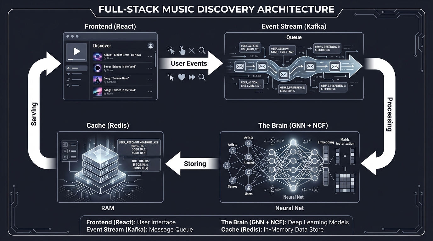
Look and Behavior:
- A “For You” rail that shifts its genres if you skip three Jazz songs in a row.
- A “Why this?” tooltip that explains the recommendation (e.g., “Because you like Miles Davis”).
- Instant “Seed-based” radio generation.
The Core Question You’re Answering
“Can I build a production-grade ecosystem that handles the entire lifecycle of a recommendation—from raw click to real-time response?”
Concepts You Must Understand First
Stop and research these before coding:
- Event-Driven Architecture
- How do you decouple the “Player” from the “Recommender”?
- Why use a message broker like Kafka?
- Real-time Feature Engineering
- How do you update a user’s “Interest Profile” in milliseconds without re-training the whole model?
- Microservices Design
- How do you scale the “Inference Service” independently of the “Metadata Service”?
Questions to Guide Your Design
Before implementing, think through these:
- Latency Budgets
- How many milliseconds are allowed for: Kafka ingestion? Embedding lookup? UI render?
- Feedback Loops
- How do you prevent the “Infinite Echo” where the UI only shows things the user just heard?
- Deployment
- How do you orchestrate 4-5 different containers (DB, Redis, API, Frontend) using Docker Compose?
Thinking Exercise
The Full Lifecycle
Trace a single click on a “Like” button:
- React sends a POST request.
- FastAPI puts a message in Kafka.
- A Consumer service reads from Kafka and updates a User-Item interaction DB.
- A separate process re-calculates the User’s top 10 neighbors.
- Redis is updated with the new top 10 tracks.
- The Frontend polls (or uses WebSockets) to refresh the “Recommended” rail.
Question:
- Where is the biggest “bottleneck” in this flow?
- How would you handle a user who “Likes” 100 songs in a minute?
The Interview Questions They’ll Ask
Prepare to answer these:
- “Describe the architecture of your recommendation platform.”
- “How do you ensure data consistency between your event stream and your recommendation cache?”
- “What happens to your system if the Kafka cluster goes down?”
- “How do you monitor the ‘Performance Drift’ of your model in production?”
Hints in Layers
Hint 1: Modularize Build the Projects 1, 8, and 13 as independent services first.
Hint 2: Use Docker Compose This is the only way to manage the 5+ services you’ll need for this project.
Hint 3: Simplify the Frontend
Don’t get bogged down in CSS. Use a library like Material UI or Tailwind to build the dashboard quickly.
Hint 4: Mock Data Use the Million Song Dataset or the Spotify Million Playlist Dataset to populate your catalog.
Books That Will Help
| Topic | Book | Chapter |
|---|---|---|
| Microservices | “Building Microservices” | Ch. 1-4 |
| Data-Intensive Apps | “Designing Data-Intensive Applications” | Ch. 11 (Stream Processing) |
| React/API Design | “Clean Architecture” | Ch. 17-22 |
Project Comparison Table
| Project | Difficulty | Time | Depth of Understanding | Fun Factor |
|---|---|---|---|---|
| #1: Content-Based | Level 1 | Weekend | Low (Foundational) | 2/5 |
| #4: Hybrid | Level 3 | 1 Week | Medium (Crucial) | 3/5 |
| #6: Matrix Fact. | Level 4 | 2 Weeks | High (The “Standard”) | 4/5 |
| #14: GNN (Graph) | Level 5 | 1 Month | Very High (Modern) | 5/5 |
| #18: Full-Stack | Level 5 | 2 Months | Total Mastery | 5/5 |
Recommendation
If you are a beginner: Start with Project #1 and #2. They build the fundamental mental model of how data represents taste.
If you are an engineer looking for a job: Focus on Project #8 (API) and Project #13 (Implicit Feedback). Companies care most about how you handle real-world, messy, high-volume data.
If you want to be a researcher: Dive deep into Project #14 (GNNs) and #17 (RL). These are where the biggest breakthroughs are happening today.
Final Overall Project: The “SoundStream” Discovery Ecosystem
This isn’t just one app; it’s a suite of services.
- The Ingestor: A Python script simulating millions of “Listen” events flowing into a Kafka topic.
- The Brain: A Hybrid model using GNNs for collaborative filtering and CNNs for audio analysis.
- The Servicer: A FastAPI endpoint containerized in Docker, backed by Redis.
- The UI: A React dashboard showing “Discovery Weekly” playlists that change dynamically as you skip songs.
Summary
This learning path covers music recommendation through 18 hands-on projects.
Recommended Learning Path
For beginners: Start with projects #1, #2, #3. For intermediate: Jump to projects #4, #6, #8. For advanced: Focus on projects #14, #15, #18.
Expected Outcomes
After completing these projects, you will:
- Understand every byte of the recommendation pipeline.
- Be able to extract “DNA” from raw sound files.
- Master the math of latent factor models and neural embeddings.
- Know how to scale an ML system to serve millions of users.
- Have a portfolio piece that rivals the engineering of top-tier streaming services.
```