P05: Recommendation Engine with Matrix Factorization
Build a movie/music recommendation system that uses matrix factorization to predict user preferences from sparse ratings data.
Overview
| Attribute | Value |
|---|---|
| Difficulty | Intermediate |
| Time Estimate | 1-2 weeks |
| Language | Python (recommended) or C |
| Prerequisites | Basic matrix operations, understanding of SVD (P02) |
| Primary Book | “Data Science for Business” by Provost & Fawcett |
Learning Objectives
By completing this project, you will:
- See sparse matrices in action - Most entries unknown, but patterns exist
- Master matrix factorization - Decompose user-item interactions
- Understand latent factors - Hidden dimensions of taste
- Apply optimization - Gradient descent for factorization
- Implement similarity measures - Dot products and cosine similarity
- Connect math to real products - How Netflix, Spotify, Amazon work
Theoretical Foundation
Part 1: The Recommendation Problem
What We’re Trying to Solve
┌────────────────────────────────────────────────────────────────┐
│                THE RATING MATRIX                               │
├────────────────────────────────────────────────────────────────┤
│                                                                │
│                    Movies                                      │
│              M₁   M₂   M₃   M₄   M₅   M₆                       │
│         U₁ [ 5    3    ?    1    ?    ? ]                      │
│         U₂ [ 4    ?    ?    1    ?    ? ]                      │
│  Users  U₃ [ 1    1    ?    5    ?    4 ]                      │
│         U₄ [ ?    ?    5    4    ?    ? ]                      │
│         U₅ [ ?    ?    4    ?    ?    5 ]                      │
│                                                                │
│  ? = unknown rating (user hasn't seen movie)                   │
│  Numbers = 1-5 star ratings                                    │
│                                                                │
│  Goal: Predict the ? values                                    │
│        Recommend highest predicted ratings                     │
│                                                                │
└────────────────────────────────────────────────────────────────┘
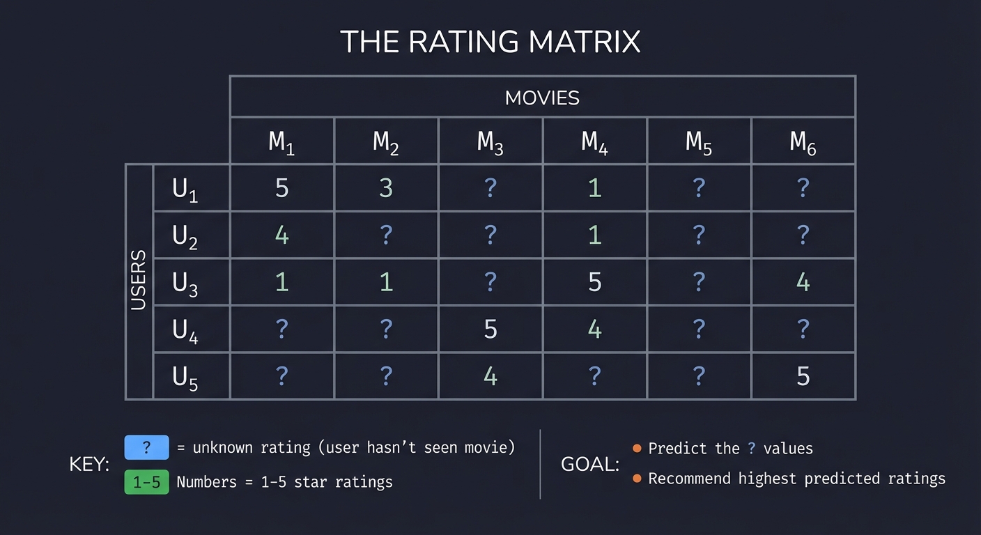
The matrix is sparse: Netflix has millions of users and thousands of movies, but each user has rated perhaps 100 movies (0.1% filled).
The Core Insight
Users who like similar things probably have similar taste. Items liked by similar users are probably similar.
If U₁ and U₂ both love action movies and hate romances, and U₁ rated M₃ highly, U₂ will probably like M₃ too.
Part 2: Matrix Factorization Intuition
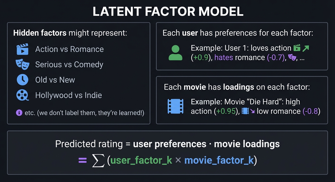
The Latent Factor Model
Assume ratings are generated by hidden (latent) factors:
┌────────────────────────────────────────────────────────────────┐
│                LATENT FACTOR MODEL                             │
├────────────────────────────────────────────────────────────────┤
│                                                                │
│   Hidden factors might represent:                              │
│   - Factor 1: Action vs Romance                                │
│   - Factor 2: Serious vs Comedy                                │
│   - Factor 3: Old vs New                                       │
│   - Factor 4: Hollywood vs Indie                               │
│   etc. (we don't label them, they're learned!)                │
│                                                                │
│   Each user has preferences for each factor:                   │
│   User 1: loves action (+0.9), hates romance (-0.7), ...      │
│                                                                │
│   Each movie has loadings on each factor:                      │
│   Movie "Die Hard": high action (+0.95), low romance (-0.8)   │
│                                                                │
│   Predicted rating = user preferences · movie loadings        │
│                    = Σ (user_factor_k × movie_factor_k)        │
│                                                                │
└────────────────────────────────────────────────────────────────┘
The Factorization
We factor the rating matrix R into two smaller matrices:
R ≈ P × Qᵀ

Where:
- R is m×n (m users, n items)
- P is m×k (m users, k factors) — user feature matrix
- Q is n×k (n items, k factors) — item feature matrix
- k << min(m, n) — typically 10-200 factors

User i's predicted rating for item j:
r̂ᵢⱼ = pᵢ · qⱼ = Σₖ pᵢₖ × qⱼₖ

This is a dot product of user and item vectors!
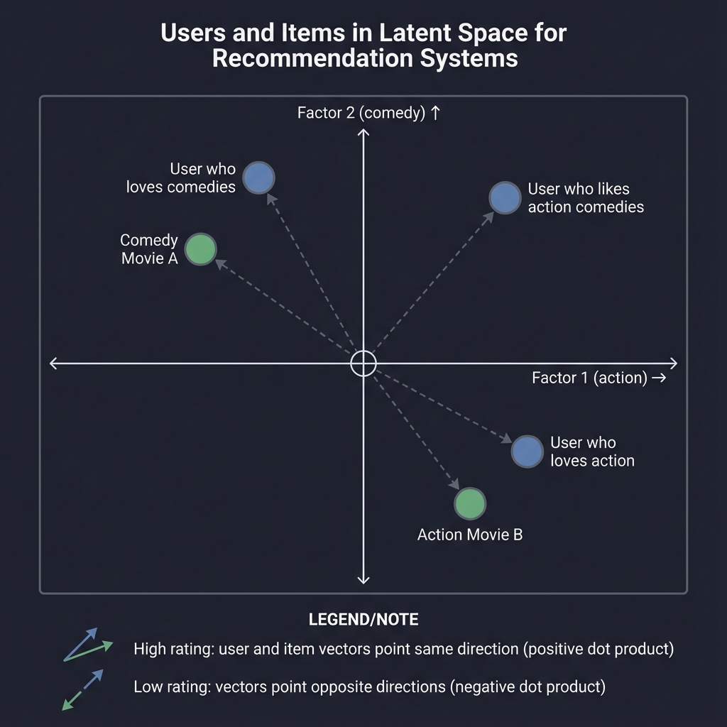
Geometrically:
┌────────────────────────────────────────────────────────────────┐
│              USERS AND ITEMS IN LATENT SPACE                   │
├────────────────────────────────────────────────────────────────┤
│                                                                │
│    Factor 2 (comedy)                                           │
│        ↑                                                       │
│        │     • Comedy Movie A                                  │
│        │   ╱  • User who loves comedies                       │
│        │ ╱                                                     │
│        │╱  • User who likes action comedies                   │
│    ────●────────────────────→ Factor 1 (action)               │
│       ╱│╲                                                      │
│      ╱ │ ╲                                                     │
│     •  │  • Action Movie B                                    │
│   User who   │                                                 │
│   loves action                                                │
│                                                                │
│   High rating when user and item vectors point same direction │
│   (large positive dot product)                                │
│                                                                │
│   Low rating when they point opposite directions              │
│   (large negative dot product)                                │
│                                                                │
└────────────────────────────────────────────────────────────────┘
Part 3: Learning the Factorization
The Objective Function
Find P and Q that minimize reconstruction error on known ratings:
minimize  Σ_(i,j)∈known [(rᵢⱼ - pᵢ·qⱼ)²] + λ(||P||² + ||Q||²)
             ↑                               ↑
        reconstruction error           regularization
                                    (prevent overfitting)
This is a non-convex optimization problem!
Stochastic Gradient Descent (SGD)
For each known rating rᵢⱼ:
# Compute error
prediction = dot(P[i], Q[j])
error = r[i,j] - prediction

# Update user and item factors
P[i] += learning_rate * (error * Q[j] - regularization * P[i])
Q[j] += learning_rate * (error * P[i] - regularization * Q[j])
Why this works:
- If we under-predict (error > 0), move P[i] and Q[j] closer together
- If we over-predict (error < 0), move them apart
- Regularization shrinks factors toward zero (prevents huge values)
Alternating Least Squares (ALS)
Alternative approach: fix one matrix, optimize the other analytically:
1. Fix P, solve for Q (least squares problem)
2. Fix Q, solve for P (least squares problem)
3. Repeat until convergence
Each step is a linear regression! More parallelizable than SGD.
Part 4: Handling Sparsity
The Challenge
Netflix has:
- ~200 million users
- ~15,000 movies
- = 3 trillion possible ratings
- But only ~5 billion actual ratings (0.17% filled!)

We can't store or operate on a dense 200M × 15K matrix.
Sparse Matrix Representation
Store only non-zero (known) values:
# Coordinate format (COO)
ratings = [
    (user_id=0, item_id=2, rating=4.5),
    (user_id=0, item_id=7, rating=3.0),
    (user_id=1, item_id=2, rating=5.0),
    ...
]

# Compressed Sparse Row (CSR) - efficient for row slicing
# Or Compressed Sparse Column (CSC) - efficient for column slicing
Training on Sparse Data
We only compute loss and updates for known ratings:
for (i, j, rating) in training_data:
    pred = dot(P[i], Q[j])
    error = rating - pred
    # Update only P[i] and Q[j]
This is efficient — we never touch the billions of unknown entries.
Part 5: Biases and Extensions
User and Item Biases
Some users rate everything high; some movies are universally loved:
r̂ᵢⱼ = μ + bᵤᵢ + bᵢⱼ + pᵢ · qⱼ

Where:
- μ = global average rating (~3.5 for 1-5 scale)
- bᵤᵢ = user i's bias (how much they deviate from average)
- bᵢⱼ = item j's bias (how much it deviates from average)
- pᵢ · qⱼ = interaction term (personalized component)
Example:
Global average: 3.5
User "harsh critic": bias = -1.0 (rates 1 star lower than average)
Movie "The Godfather": bias = +1.5 (rated 1.5 stars higher)
Interaction: +0.3 (this user especially likes this genre)

Prediction: 3.5 + (-1.0) + 1.5 + 0.3 = 4.3 stars
Implicit Feedback
Not just explicit ratings — consider views, clicks, purchases:
R = explicit ratings (sparse)
C = confidence matrix (dense, based on implicit data)

Higher confidence for items with more interaction:
c_ij = 1 + α × (number of times user i interacted with item j)
This is the basis of ALS for Implicit Feedback (iALS).
Part 6: Similarity Measures
Cosine Similarity
How similar are two vectors? Measure the angle between them:
cosine(u, v) = (u · v) / (||u|| × ||v||)

Range: [-1, 1]
- 1: identical direction (perfectly similar)
- 0: perpendicular (unrelated)
- -1: opposite (perfectly dissimilar)
For recommendation:
def find_similar_items(item_id, Q, k=10):
    """Find k most similar items based on latent factors."""
    target = Q[item_id]
    similarities = []
    for other_id in range(len(Q)):
        if other_id != item_id:
            sim = cosine_similarity(target, Q[other_id])
            similarities.append((other_id, sim))
    return sorted(similarities, key=lambda x: -x[1])[:k]
Euclidean Distance
Alternative: measure straight-line distance:
distance(u, v) = ||u - v|| = √Σ(uᵢ - vᵢ)²

Closer = more similar
Can convert to similarity: sim = 1 / (1 + distance)
When to Use Which
Cosine similarity:
- Ignores magnitude (user who rates 1-5 similar to user who rates 3-5)
- Good when direction matters more than scale

Euclidean distance:
- Sensitive to magnitude
- Good when absolute values matter

Pearson correlation:
- Cosine similarity of mean-centered vectors
- Handles different rating scales
Part 7: Evaluation Metrics
Root Mean Square Error (RMSE)
RMSE = √[(1/n) × Σ(rᵢⱼ - r̂ᵢⱼ)²]

Lower is better. On 1-5 scale:
- RMSE < 0.8: Excellent
- RMSE 0.8-0.9: Good
- RMSE 0.9-1.0: Acceptable
- RMSE > 1.0: Poor
Mean Absolute Error (MAE)
MAE = (1/n) × Σ|rᵢⱼ - r̂ᵢⱼ|

Easier to interpret: "on average, predictions are off by X stars"
Ranking Metrics
For recommendations, ranking often matters more than exact ratings:
Precision@K: Of top K recommended items, how many are relevant?
Recall@K:    Of all relevant items, how many are in top K?
NDCG:        Normalized Discounted Cumulative Gain (position-aware)
Train/Test Split
Critical: Don’t leak future data!
# Random split
train, test = random_split(ratings, 0.8)

# Temporal split (more realistic)
train = ratings[ratings['timestamp'] < cutoff]
test = ratings[ratings['timestamp'] >= cutoff]

# Leave-one-out
For each user, hold out one rating for testing
Part 8: Cold Start Problem
The Challenge
New users or new items have no ratings — how do we recommend?
New User:
- No ratings → no user vector P[i]
- Can't compute pᵢ · qⱼ for any item

New Item:
- No ratings → no item vector Q[j]
- Can't compute pᵢ · qⱼ for any user
Solutions
For cold-start users:
- Ask for initial preferences (onboarding)
- Use demographic features (age, location)
- Show popular items until enough data
For cold-start items:
- Use content features (genre, actors, description)
- Show to diverse users for exploration
- Hybrid: combine collaborative filtering with content-based
Content-augmented factorization:
pᵢ = P[i] + Σ(user features)
qⱼ = Q[j] + Σ(item features)

Now even new items have a representation from their features!
Part 9: Connection to SVD
Relationship
Matrix factorization for recommendations is related to SVD:
SVD:  R = U × Σ × Vᵀ    (exact decomposition)

MF:   R ≈ P × Qᵀ        (approximate, learns from data)

P roughly corresponds to U × √Σ
Q roughly corresponds to V × √Σ
Key differences:
- SVD requires knowing all entries (or imputation)
- MF optimizes only on known entries
- MF can incorporate regularization, biases, etc.
- MF is directly optimized for prediction, not reconstruction
Truncated SVD for Recommendation
You can use SVD for recommendations:
- Fill unknown entries (with zeros, mean, or imputed values)
- Compute SVD
- Keep top k singular values/vectors
- Predict with truncated matrices
But this is less effective than training directly on the sparse loss.
Project Specification
What You’re Building
A recommendation system that:
- Loads user-item rating data
- Learns latent factor representations
- Predicts ratings for unseen items
- Recommends top-N items for each user
- Evaluates predictions with RMSE/MAE
Minimum Requirements
- Load and parse MovieLens dataset
- Implement matrix factorization with SGD
- Include user and item biases
- Regularization to prevent overfitting
- Train/test split for evaluation
- Report RMSE on test set
- Generate top-N recommendations for users
Stretch Goals
- Implement ALS as alternative training method
- Add time-aware recommendations
- Implement content-based features (genres)
- Build simple web interface
- Compare with baseline methods
Solution Architecture
Data Structures
class MatrixFactorization:
    def __init__(self, n_users: int, n_items: int, n_factors: int):
        # Latent factor matrices
        self.P = np.random.normal(0, 0.1, (n_users, n_factors))
        self.Q = np.random.normal(0, 0.1, (n_items, n_factors))

        # Biases
        self.user_bias = np.zeros(n_users)
        self.item_bias = np.zeros(n_items)
        self.global_mean = 0

    def predict(self, user_id: int, item_id: int) -> float:
        """Predict rating for user-item pair."""
        pass

    def fit(self, ratings: list, epochs: int, lr: float, reg: float):
        """Train on list of (user, item, rating) tuples."""
        pass

    def recommend(self, user_id: int, n: int = 10) -> list:
        """Get top N recommendations for user."""
        pass
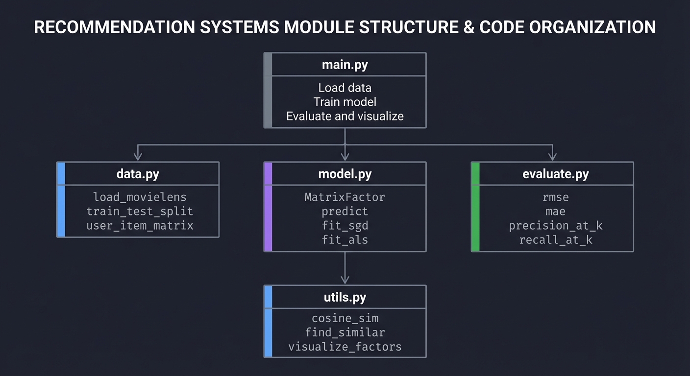
Module Structure
┌─────────────────────────────────────────────────────────────────┐
│                           main.py                               │
│  - Load data                                                    │
│  - Train model                                                  │
│  - Evaluate and visualize                                       │
└─────────────────────────────────────────────────────────────────┘
                               │
        ┌──────────────────────┼──────────────────────┐
        ▼                      ▼                      ▼
┌──────────────┐      ┌──────────────┐      ┌──────────────┐
│   data.py    │      │   model.py   │      │  evaluate.py │
│              │      │              │      │              │
│ load_movielens│     │ MatrixFactor │      │ rmse         │
│ train_test_split│   │ predict      │      │ mae          │
│ user_item_matrix│   │ fit_sgd      │      │ precision_at_k│
│              │      │ fit_als      │      │ recall_at_k  │
└──────────────┘      └──────────────┘      └──────────────┘
                               │
                               ▼
                      ┌──────────────┐
                      │  utils.py    │
                      │              │
                      │ cosine_sim   │
                      │ find_similar │
                      │ visualize_factors │
                      └──────────────┘
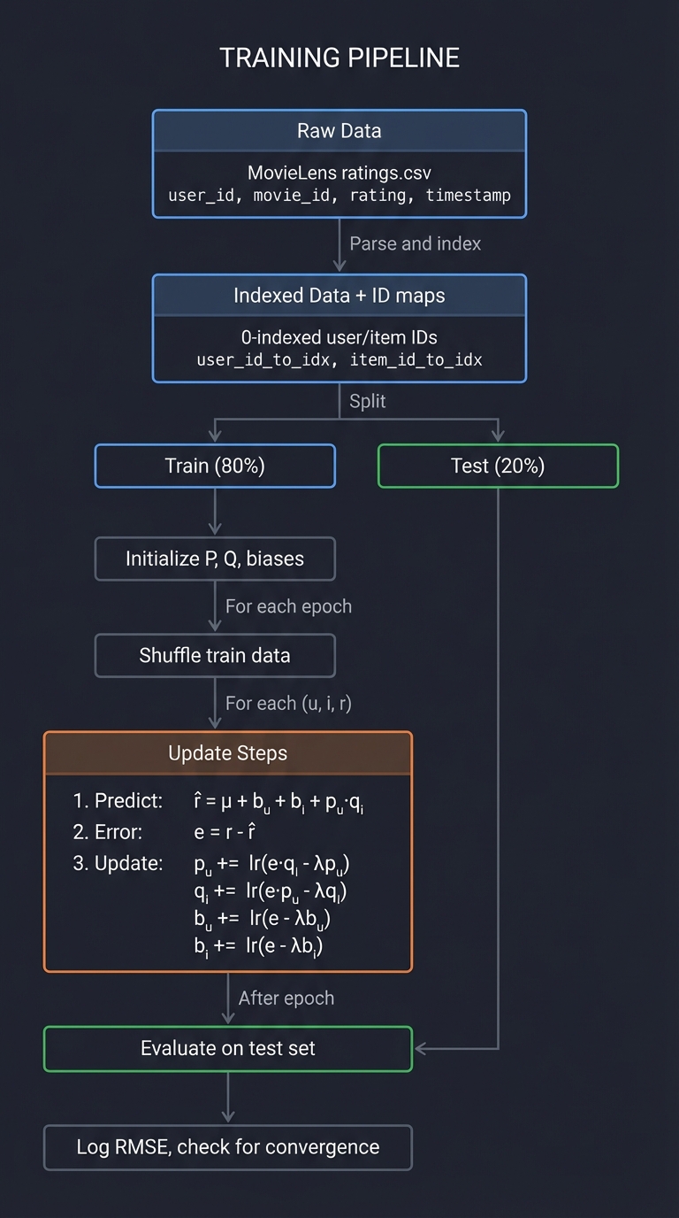
Training Pipeline
┌─────────────────────────────────────────────────────────────────────────┐
│                      TRAINING PIPELINE                                 │
├─────────────────────────────────────────────────────────────────────────┤
│                                                                         │
│  ┌─────────────┐                                                        │
│  │ Raw Data    │  MovieLens ratings.csv                                │
│  │ (u, i, r, t)│  user_id, movie_id, rating, timestamp                 │
│  └──────┬──────┘                                                        │
│         │                                                               │
│         ▼  Parse and index                                              │
│  ┌─────────────┐                                                        │
│  │ Indexed Data│  (0-indexed user/item IDs)                            │
│  │ + ID maps   │  user_id_to_idx, item_id_to_idx                       │
│  └──────┬──────┘                                                        │
│         │                                                               │
│         ▼  Split                                                        │
│  ┌─────────────────────────────────────────────────────────────┐       │
│  │ Train (80%)           │         Test (20%)                   │       │
│  └──────┬────────────────┴────────────┬────────────────────────┘       │
│         │                              │                                │
│         ▼                              │                                │
│  ┌─────────────┐                       │                                │
│  │ Initialize  │                       │                                │
│  │ P, Q, biases│                       │                                │
│  └──────┬──────┘                       │                                │
│         │                              │                                │
│         ▼  For each epoch              │                                │
│  ┌─────────────┐                       │                                │
│  │ Shuffle     │                       │                                │
│  │ train data  │                       │                                │
│  └──────┬──────┘                       │                                │
│         │                              │                                │
│         ▼  For each (u, i, r)          │                                │
│  ┌─────────────────────────────────────┼─────────────────────────────┐ │
│  │ 1. Predict: r̂ = μ + bᵤ + bᵢ + pᵤ·qᵢ │                             │ │
│  │ 2. Error:   e = r - r̂               │                             │ │
│  │ 3. Update:  pᵤ += lr(e·qᵢ - λpᵤ)    │                             │ │
│  │             qᵢ += lr(e·pᵤ - λqᵢ)    │                             │ │
│  │             bᵤ += lr(e - λbᵤ)       │                             │ │
│  │             bᵢ += lr(e - λbᵢ)       │                             │ │
│  └─────────────────────────────────────┼─────────────────────────────┘ │
│         │                              │                                │
│         ▼  After epoch                 │                                │
│  ┌─────────────┐                       │                                │
│  │ Evaluate on │◀──────────────────────┘                                │
│  │ test set    │                                                        │
│  └──────┬──────┘                                                        │
│         │                                                               │
│         ▼                                                               │
│  ┌─────────────┐                                                        │
│  │ Log RMSE,   │                                                        │
│  │ check for   │                                                        │
│  │ convergence │                                                        │
│  └─────────────┘                                                        │
│                                                                         │
└─────────────────────────────────────────────────────────────────────────┘
Phased Implementation Guide
Phase 1: Data Loading (Days 1-2)
Goal: Load and explore MovieLens dataset
Tasks:
- Download MovieLens 100K or 1M dataset
- Parse CSV files (ratings, movies, users)
- Create user/item ID mappings
- Explore data statistics
Implementation:
def load_movielens(path):
    """Load MovieLens dataset."""
    ratings = pd.read_csv(
        f"{path}/ratings.csv",
        names=['user_id', 'item_id', 'rating', 'timestamp']
    )

    # Create mappings to 0-indexed IDs
    user_ids = ratings['user_id'].unique()
    item_ids = ratings['item_id'].unique()

    user_to_idx = {u: i for i, u in enumerate(user_ids)}
    item_to_idx = {i: j for j, i in enumerate(item_ids)}

    # Convert to tuples
    data = [
        (user_to_idx[r.user_id], item_to_idx[r.item_id], r.rating)
        for r in ratings.itertuples()
    ]

    return data, user_to_idx, item_to_idx
Verification:
- Correct number of users/items
- Rating distribution looks reasonable (1-5 scale)
- No missing or invalid data
Phase 2: Basic Matrix Factorization (Days 3-5)
Goal: Implement core prediction and training
Tasks:
- Initialize P and Q matrices randomly
- Implement prediction function
- Implement SGD update step
- Train on small subset first
Implementation:
class MatrixFactorization:
    def __init__(self, n_users, n_items, n_factors=10):
        # Initialize with small random values
        self.P = np.random.normal(0, 0.1, (n_users, n_factors))
        self.Q = np.random.normal(0, 0.1, (n_items, n_factors))

    def predict(self, u, i):
        return np.dot(self.P[u], self.Q[i])

    def train_step(self, u, i, r, lr=0.01, reg=0.02):
        pred = self.predict(u, i)
        error = r - pred

        # Gradient descent update
        p_update = lr * (error * self.Q[i] - reg * self.P[u])
        q_update = lr * (error * self.P[u] - reg * self.Q[i])

        self.P[u] += p_update
        self.Q[i] += q_update

        return error ** 2
Verification:
- Loss decreases over epochs
- Predictions are in reasonable range
- No NaN or inf values
Phase 3: Biases and Global Mean (Days 6-7)
Goal: Add bias terms for better predictions
Tasks:
- Compute global mean rating
- Add user bias array
- Add item bias array
- Update training to include biases
Implementation:
class MatrixFactorization:
    def __init__(self, n_users, n_items, n_factors=10):
        self.P = np.random.normal(0, 0.1, (n_users, n_factors))
        self.Q = np.random.normal(0, 0.1, (n_items, n_factors))
        self.user_bias = np.zeros(n_users)
        self.item_bias = np.zeros(n_items)
        self.global_mean = 0

    def predict(self, u, i):
        return (self.global_mean +
                self.user_bias[u] +
                self.item_bias[i] +
                np.dot(self.P[u], self.Q[i]))

    def train_step(self, u, i, r, lr=0.01, reg=0.02):
        pred = self.predict(u, i)
        error = r - pred

        # Update biases
        self.user_bias[u] += lr * (error - reg * self.user_bias[u])
        self.item_bias[i] += lr * (error - reg * self.item_bias[i])

        # Update factors
        p_update = lr * (error * self.Q[i] - reg * self.P[u])
        q_update = lr * (error * self.P[u] - reg * self.Q[i])
        self.P[u] += p_update
        self.Q[i] += q_update

        return error ** 2
Verification:
- Biases capture user/item tendencies
- RMSE improves with biases
- High-rated items have positive item bias
Phase 4: Evaluation (Days 8-9)
Goal: Properly evaluate model performance
Tasks:
- Implement train/test split
- Implement RMSE and MAE
- Track metrics over epochs
- Plot learning curves
Implementation:
def train_test_split(data, test_ratio=0.2):
    """Random split of ratings."""
    np.random.shuffle(data)
    split = int(len(data) * (1 - test_ratio))
    return data[:split], data[split:]

def evaluate(model, test_data):
    """Compute RMSE on test set."""
    squared_errors = []
    for u, i, r in test_data:
        pred = model.predict(u, i)
        squared_errors.append((r - pred) ** 2)
    return np.sqrt(np.mean(squared_errors))

def train(model, train_data, test_data, epochs=20, lr=0.01, reg=0.02):
    """Training loop with evaluation."""
    for epoch in range(epochs):
        np.random.shuffle(train_data)
        total_loss = 0

        for u, i, r in train_data:
            total_loss += model.train_step(u, i, r, lr, reg)

        train_rmse = np.sqrt(total_loss / len(train_data))
        test_rmse = evaluate(model, test_data)
        print(f"Epoch {epoch}: Train RMSE={train_rmse:.4f}, Test RMSE={test_rmse:.4f}")
Verification:
- Test RMSE is reasonable (< 1.0)
- Training loss decreases
- No overfitting (test RMSE doesn’t increase much)
Phase 5: Recommendation Generation (Days 10-11)
Goal: Generate personalized recommendations
Tasks:
- Find items user hasn’t rated
- Predict ratings for all unseen items
- Return top-N recommendations
- Show movie titles with predictions
Implementation:
def get_recommendations(model, user_id, user_rated_items, all_items, n=10):
    """Get top N recommendations for user."""
    unseen = set(all_items) - set(user_rated_items[user_id])

    predictions = []
    for item_id in unseen:
        pred = model.predict(user_id, item_id)
        predictions.append((item_id, pred))

    # Sort by predicted rating, descending
    predictions.sort(key=lambda x: -x[1])

    return predictions[:n]

# Usage
recs = get_recommendations(model, user_id=42, user_rated_items, all_items, n=10)
for item_id, pred_rating in recs:
    print(f"{movie_titles[item_id]}: {pred_rating:.2f} stars (predicted)")
Verification:
- Recommendations make intuitive sense
- User’s highly-rated genres appear in recommendations
- No already-rated items in recommendations
Phase 6: Similarity and Exploration (Days 12-14)
Goal: Find similar items and interpret factors
Tasks:
- Implement cosine similarity
- Find similar items/users
- Visualize latent factors
- Interpret what factors might mean
Implementation:
def cosine_similarity(v1, v2):
    """Compute cosine similarity between two vectors."""
    dot = np.dot(v1, v2)
    norm1 = np.linalg.norm(v1)
    norm2 = np.linalg.norm(v2)
    return dot / (norm1 * norm2 + 1e-8)

def find_similar_items(model, item_id, k=10):
    """Find k most similar items based on latent factors."""
    target = model.Q[item_id]
    similarities = []

    for other_id in range(len(model.Q)):
        if other_id != item_id:
            sim = cosine_similarity(target, model.Q[other_id])
            similarities.append((other_id, sim))

    return sorted(similarities, key=lambda x: -x[1])[:k]

def visualize_factors(model, item_ids, item_names, factors=[0, 1]):
    """Plot items in 2D factor space."""
    plt.figure(figsize=(10, 8))
    for item_id in item_ids:
        x = model.Q[item_id, factors[0]]
        y = model.Q[item_id, factors[1]]
        plt.scatter(x, y)
        plt.annotate(item_names[item_id][:20], (x, y))
    plt.xlabel(f"Factor {factors[0]}")
    plt.ylabel(f"Factor {factors[1]}")
    plt.show()
Verification:
- Similar items by similarity are sensibly related
- Factors show clustering by genre
- Visualization reveals interpretable structure
Testing Strategy
Unit Tests
- Data loading:
- Correct number of ratings loaded
- All ratings in valid range (1-5)
- ID mappings are bijective
- Model components:
- Prediction is dot product plus biases
- Updates change P and Q
- Regularization shrinks factors
- Metrics:
- RMSE of constant prediction equals std deviation
- Perfect predictions give RMSE of 0
Integration Tests
- Overfitting test: Can model achieve near-zero loss on small dataset?
- Bias test: Does adding biases improve RMSE?
- Regularization test: Does reg prevent overfitting?
Sanity Checks
- Known item similarity: Do “Star Wars” and “Empire Strikes Back” have high similarity?
- User consistency: If user rates action movies high, do action movies appear in recommendations?
- Extreme predictions: Are all predictions in reasonable range (1-5)?
Common Pitfalls and Debugging
Learning Rate Issues
Symptom: Loss oscillates or diverges
Cause: Learning rate too high
Fix: Start with lr=0.001, increase gradually
Regularization Issues
Symptom: Test RMSE much higher than train RMSE
Cause: Overfitting (regularization too low)
Fix: Increase λ (try 0.02, 0.05, 0.1)
Cold Start Errors
Symptom: Errors on new users/items
Cause: User/item not in training data
Fix: Use fallback (global mean, popular items)
Numerical Issues
Symptom: NaN in predictions or loss
Cause: Division by zero, overflow
Fix: Add epsilon to denominators, clip values
Slow Training
Symptom: Hours to train on MovieLens 1M
Cause: Pure Python loops
Fix: Vectorize, use NumPy, or implement in C
Extensions and Challenges
Beginner Extensions
- Tune hyperparameters (factors, lr, reg)
- Add early stopping
- Save/load trained model
Intermediate Extensions
- Implement ALS instead of SGD
- Add temporal dynamics (ratings change over time)
- Incorporate item genres as features
- Build a simple web demo
Advanced Extensions
- Implement implicit feedback model
- Add side information (user demographics)
- Neural collaborative filtering
- A/B testing simulation
Real-World Connections
Netflix
The Netflix Prize (2006-2009) popularized matrix factorization:
- $1 million for 10% improvement in RMSE
- Winning solution: ensemble of many models, MF as core
- Showed practical value of latent factor models
Spotify
Uses collaborative filtering for:
- Discover Weekly playlist
- Related artists
- Radio stations
Plus content features (audio analysis).
Amazon
“Customers who bought X also bought Y”:
- Item-item collaborative filtering
- Fast to compute (precomputed similarities)
- Core of product recommendation
YouTube
Deep learning + collaborative filtering:
- Candidate generation (MF-like)
- Ranking (deep neural network)
- Billions of users and videos
Self-Assessment Checklist
Conceptual Understanding
- I can explain what latent factors represent
- I understand why the dot product measures preference
- I know how biases improve predictions
- I can explain the cold start problem
- I understand the tradeoff between bias and variance
Practical Skills
- I implemented matrix factorization with SGD
- My model achieves reasonable RMSE (< 0.95 on MovieLens)
- I can generate and interpret recommendations
- I can find similar items using learned factors
- I can tune hyperparameters effectively
Teaching Test
Can you explain to someone else:
- Why do we factorize the rating matrix?
- What do the user and item vectors represent?
- How does training work?
- Why is regularization important?
Resources
Primary
- “Data Science for Business” by Provost & Fawcett - Business context
- “Recommender Systems Handbook” - Comprehensive reference
- Netflix Prize papers - Original inspiration
Reference
- Surprise library - Python recommendation toolkit
- LightFM - Hybrid recommendation library
- MovieLens datasets - Standard benchmarks
Online
- Google’s Recommendation ML course - Practical guide
- Koren et al. “Matrix Factorization Techniques” - Classic paper
- Coursera: Recommender Systems Specialization - Academic depth
When you complete this project, you’ll understand that recommendation systems are applied linear algebra—users and items as vectors, preferences as dot products, learning as optimization. Every time Netflix suggests a movie, this math is running behind the scenes.