P04: Physics Simulation with Constraints
Build a 2D physics engine that simulates rigid body dynamics with constraints (springs, joints, collisions)—requiring you to solve systems of linear equations each frame.
Overview
| Attribute | Value |
|---|---|
| Difficulty | Advanced |
| Time Estimate | 3-4 weeks |
| Language | C (recommended) or Python |
| Prerequisites | Basic physics intuition, matrix operations |
| Primary Book | “Game Physics Engine Development” by Ian Millington |
Learning Objectives
By completing this project, you will:
- See vectors as physical state - Position, velocity, and acceleration as mathematical objects
- Master Ax = b solvers - Gaussian elimination and iterative methods
- Understand projections geometrically - Collision response via vector projection
- Grasp matrix conditioning - Why some systems are “hard” to solve
- Apply null spaces and least squares - Handle over/under-constrained systems
- Experience numerical stability - When math works on paper but fails in code
Theoretical Foundation
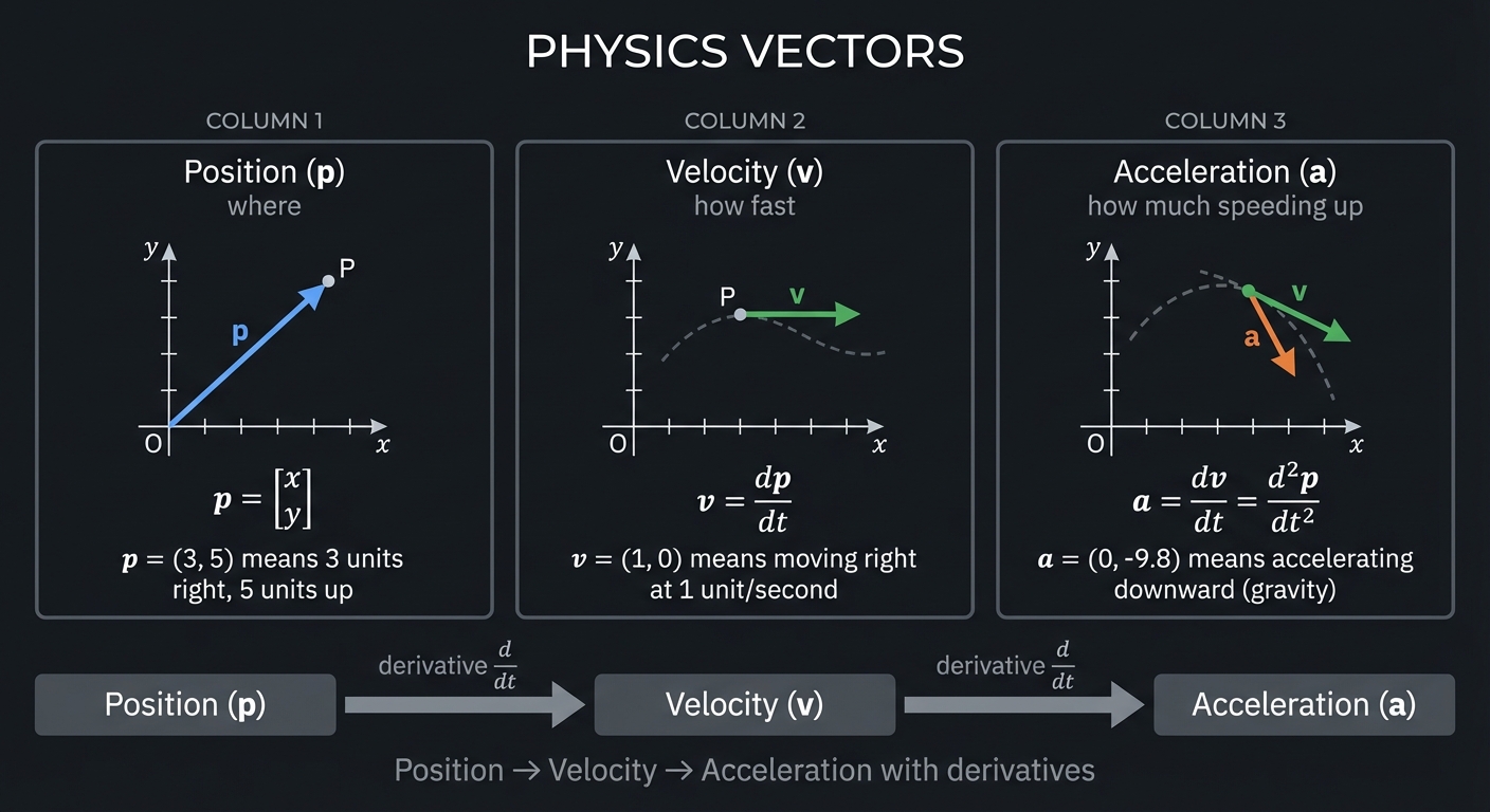
Part 1: Vectors as Physical State
Position, Velocity, Acceleration
Every physics simulation begins with vectors representing physical quantities:
┌────────────────────────────────────────────────────────────────┐
│                    PHYSICS VECTORS                             │
├────────────────────────────────────────────────────────────────┤
│                                                                │
│    Position (p)     Velocity (v)     Acceleration (a)         │
│    "where"          "how fast"       "how much speeding up"   │
│                                                                │
│    p = [x]          v = dp/dt        a = dv/dt = d²p/dt²      │
│        [y]                                                     │
│                                                                │
│    For a 2D point:                                             │
│    p = (3, 5) means 3 units right, 5 units up                 │
│    v = (1, 0) means moving right at 1 unit/second             │
│    a = (0, -9.8) means accelerating downward (gravity)        │
│                                                                │
└────────────────────────────────────────────────────────────────┘
Newton’s Second Law in Vector Form
F = ma

Force vector → acceleration vector → velocity change → position change

For multiple forces:
a = (1/m) × ΣF = (1/m) × (F_gravity + F_spring + F_collision + ...)

Each force is a vector; we sum them.
The State Vector
For a system of n particles, collect all positions and velocities:
State vector S:

    [p₁]     position of particle 1
    [p₂]     position of particle 2
S = [...]
    [v₁]     velocity of particle 1
    [v₂]     velocity of particle 2
    [...]

For n particles in 2D: S has 4n components (2 position + 2 velocity each)
This state vector evolves over time according to physics equations.
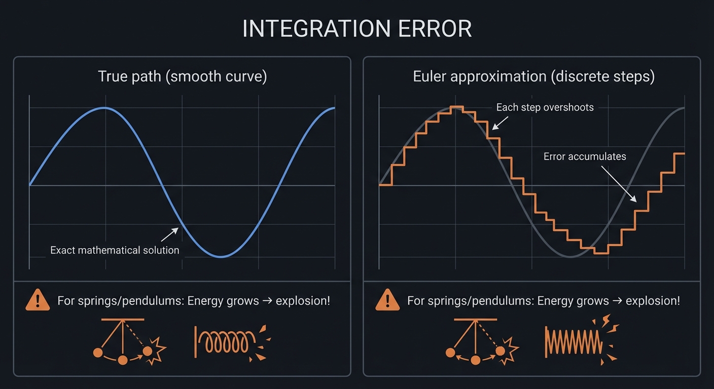
Part 2: Numerical Integration
The Euler Method
The simplest integration scheme:
v_new = v_old + a × Δt
p_new = p_old + v_old × Δt

Or more accurately (semi-implicit Euler):
v_new = v_old + a × Δt
p_new = p_old + v_new × Δt  ← use new velocity
Euler is simple but unstable - errors accumulate, springs explode.
Why Integration is Tricky
┌────────────────────────────────────────────────────────────────┐
│                    INTEGRATION ERROR                           │
├────────────────────────────────────────────────────────────────┤
│                                                                │
│    True path                   Euler approximation             │
│                                                                │
│       ╭──────╮                    ╭────────────╮               │
│      ╱        ╲                  ╱              ╲              │
│     ╱          ╲                ╱                ╲             │
│    ╱            ╲              ╱                  ╲            │
│                                      ↑                         │
│                           Each step overshoots                 │
│                           Error accumulates                    │
│                                                                │
│   For springs/pendulums: Energy grows → explosion!            │
│                                                                │
└────────────────────────────────────────────────────────────────┘
Better Methods: Verlet Integration
Position-based method that conserves energy better:
p_new = 2×p_current - p_old + a × Δt²

Velocity is implicit: v ≈ (p_new - p_old) / (2×Δt)

Advantages:
- Second-order accurate (error ∝ Δt²)
- Energy-conserving (symplectic)
- Simple to implement
RK4 (Runge-Kutta 4th Order)
More accurate but expensive:
k₁ = f(t, y)
k₂ = f(t + Δt/2, y + Δt×k₁/2)
k₃ = f(t + Δt/2, y + Δt×k₂/2)
k₄ = f(t + Δt, y + Δt×k₃)

y_new = y + (Δt/6) × (k₁ + 2k₂ + 2k₃ + k₄)
For this project, semi-implicit Euler or Verlet is sufficient.
Part 3: Collision Detection and Response
Detecting Collisions
For circles, collision detection is simple:
Circle A: center pA, radius rA
Circle B: center pB, radius rB

Distance: d = ||pA - pB||
Collision: d < rA + rB

Penetration depth: δ = (rA + rB) - d
Collision normal: n = (pB - pA) / d
For boxes, polygons, etc., it gets more complex (SAT, GJK).
Collision Response via Projection
The key linear algebra insight: collision response is projection!
┌────────────────────────────────────────────────────────────────┐
│                 COLLISION RESPONSE                             │
├────────────────────────────────────────────────────────────────┤
│                                                                │
│    Before collision:                                           │
│                                                                │
│         v (incoming velocity)                                  │
│          ↘                                                     │
│           ↘                                                    │
│    ─────────●───────── surface (normal n)                      │
│                                                                │
│    Decompose v into components:                                │
│                                                                │
│    v_normal = (v · n) × n     (component along normal)         │
│    v_tangent = v - v_normal   (component along surface)        │
│                                                                │
│    For elastic bounce:                                         │
│    v_new = v_tangent - e × v_normal  (e = coefficient of      │
│                                        restitution)            │
│                                                                │
│    For e = 1 (perfectly elastic):                              │
│    v_new = v - 2(v · n)n      (reflection formula)            │
│                                                                │
└────────────────────────────────────────────────────────────────┘
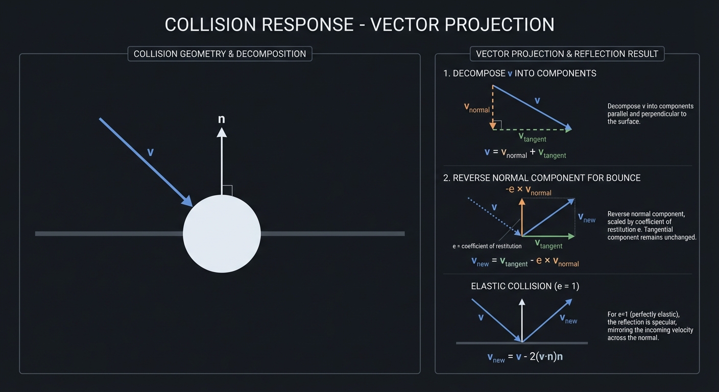
The math:
Reflection: v_reflected = v - 2(v · n)n

This is the formula for reflecting a vector across a plane!
The dot product measures how much v points into the surface.
Multiplying by n and subtracting reverses that component.
Impulse-Based Collision
For realistic physics, we compute impulses (instantaneous momentum changes):
For two colliding bodies A and B:

Relative velocity: v_rel = vA - vB
Normal component:  v_n = v_rel · n

If v_n > 0: bodies separating, no collision response needed

Impulse magnitude: j = -(1 + e) × v_n / (1/mA + 1/mB)

Apply impulse:
vA_new = vA + (j/mA) × n
vB_new = vB - (j/mB) × n
Part 4: Constraints and Solving Ax = b
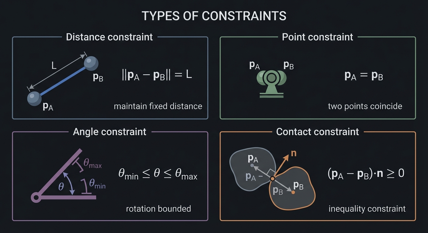
What is a Constraint?
A constraint is a restriction on how bodies can move:
┌────────────────────────────────────────────────────────────────┐
│                    TYPES OF CONSTRAINTS                        │
├────────────────────────────────────────────────────────────────┤
│                                                                │
│    Distance constraint (rod/rope):                             │
│    ||pA - pB|| = L   (maintain fixed distance)                 │
│                                                                │
│    Point constraint (pin joint):                               │
│    pA = pB           (two points coincide)                     │
│                                                                │
│    Angle constraint (hinge limit):                             │
│    θ_min ≤ θ ≤ θ_max (rotation bounded)                        │
│                                                                │
│    Contact constraint (no penetration):                        │
│    (pA - pB) · n ≥ 0  (inequality constraint)                  │
│                                                                │
└────────────────────────────────────────────────────────────────┘
Constraint Equations
Most constraints can be written as: C(x) = 0
For a distance constraint between particles at p₁ and p₂:
C = ||p₁ - p₂||² - L² = 0
Taking the derivative (for velocity-level constraint):
Ċ = 2(p₁ - p₂) · (v₁ - v₂) = 0

This says: relative velocity must be perpendicular to the connecting line.
The Jacobian Matrix
For multiple constraints on multiple bodies, we form the Jacobian:
C = [C₁]      Jacobian J = [∂C₁/∂x₁  ∂C₁/∂x₂  ...]
    [C₂]                   [∂C₂/∂x₁  ∂C₂/∂x₂  ...]
    [...]                  [  ...      ...     ...]

The constraint becomes: J × v = 0  (or = -baumgarte × C for stability)

Where v is the velocity vector of all bodies.
Solving for Constraint Forces
To satisfy constraints, we need forces. The constraint force λ:
Total acceleration: a = M⁻¹(F_external + Jᵀλ)

Constraint: J × a = b  (where b comes from the constraint)

Substituting:
J × M⁻¹ × Jᵀ × λ = b - J × M⁻¹ × F_external

This is a system:  A × λ = b

Where A = J × M⁻¹ × Jᵀ (the constraint mass matrix)
This is the heart of constraint solving: solve Ax = b to find λ, then apply forces.
Part 5: Solving Systems of Linear Equations
The General Problem
A × x = b

Given: A (n×n matrix), b (n vector)
Find:  x (n vector)
For physics:
- A encodes how constraints couple to each other
- b encodes how much the constraints are violated
- x (λ) gives the correction forces
Gaussian Elimination
The classic direct method:
Step 1: Forward elimination (create upper triangular form)
Step 2: Back substitution (solve from bottom up)

Example:
[2  1  1 | 8]     [2  1  1 | 8]     [2  1  1 | 8]
[4  3  3 | 20] →  [0  1  1 | 4] →   [0  1  1 | 4]
[8  7  9 | 46]    [0  3  5 | 14]    [0  0  2 | 2]

Back substitute: z = 1, y = 3, x = 2
Complexity: O(n³) - too slow for large systems every frame!
LU Decomposition
Factor A once, solve quickly for different b:
A = L × U  (Lower triangular × Upper triangular)

Solve: L × y = b  (forward substitution)
Then:  U × x = y  (back substitution)

Both steps are O(n²).
Useful when A doesn’t change (same constraints, different forces).
Iterative Methods: Gauss-Seidel
For constraint solving, iterative methods work well:
def gauss_seidel(A, b, x, iterations):
    for _ in range(iterations):
        for i in range(n):
            sigma = sum(A[i][j] * x[j] for j in range(n) if j != i)
            x[i] = (b[i] - sigma) / A[i][i]
    return x
Why iterative works for physics:
- Constraints are local (sparse matrix)
- Approximate solution is often good enough
- We solve many times per second (converges over frames)
Projected Gauss-Seidel (PGS)
For inequality constraints (contacts), clamp solutions:
def pgs(A, b, x, lo, hi, iterations):
    for _ in range(iterations):
        for i in range(n):
            delta = (b[i] - sum(A[i][j] * x[j] for j in range(n))) / A[i][i]
            x[i] = clamp(x[i] + delta, lo[i], hi[i])
    return x
This handles: “bodies can push apart but not pull together”
Part 6: Matrix Conditioning and Numerical Stability
What is Condition Number?
The condition number κ(A) measures how sensitive Ax = b is to perturbations:
If κ(A) is small (close to 1): well-conditioned, stable
If κ(A) is large: ill-conditioned, small errors → large errors

κ(A) = ||A|| × ||A⁻¹|| = σ_max / σ_min  (ratio of singular values)
Why Conditioning Matters for Physics
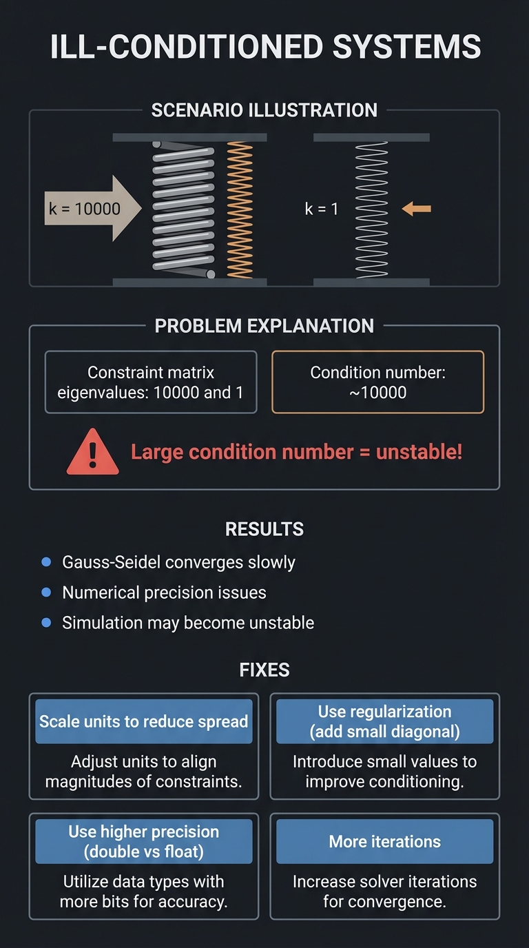
┌────────────────────────────────────────────────────────────────┐
│                ILL-CONDITIONED SYSTEMS                         │
├────────────────────────────────────────────────────────────────┤
│                                                                │
│    Scenario: Very stiff springs mixed with soft springs        │
│                                                                │
│    Stiff spring: k = 10000                                     │
│    Soft spring:  k = 1                                         │
│                                                                │
│    Constraint matrix eigenvalues: 10000 and 1                  │
│    Condition number: ~10000                                    │
│                                                                │
│    Result: Gauss-Seidel converges slowly                       │
│            Numerical precision issues                          │
│            Simulation may become unstable                      │
│                                                                │
│    Fixes:                                                      │
│    - Scale units to reduce spread                              │
│    - Use regularization (add small diagonal)                   │
│    - Use higher precision (double instead of float)            │
│    - More iterations                                           │
│                                                                │
└────────────────────────────────────────────────────────────────┘
Numerical Stability Tips
- Use double precision for constraint solving
- Add bias/regularization: A + εI instead of A
- Warm starting: Use previous frame’s solution as initial guess
- Scale appropriately: Keep values in reasonable ranges
Part 7: Special Matrix Structures
Sparse Matrices
Physics matrices are typically sparse (mostly zeros):
For a chain of particles connected by springs:

[×  ×  0  0  0  0]    × = non-zero
[×  ×  ×  0  0  0]    0 = zero
[0  ×  ×  ×  0  0]
[0  0  ×  ×  ×  0]    Each particle only interacts with neighbors.
[0  0  0  ×  ×  ×]
[0  0  0  0  ×  ×]

Store only non-zeros → memory efficient
Skip zero multiplications → faster solving
Symmetric Positive Definite (SPD)
Many physics matrices are SPD:
- Symmetric: A = Aᵀ
- Positive definite: xᵀAx > 0 for all x ≠ 0
SPD matrices have:
- All positive eigenvalues
- Cholesky factorization: A = LLᵀ (faster than LU)
- Guaranteed convergence for iterative methods
Block Structure
For rigid bodies, matrices have block structure:
[M₁  0   0 ]   [v₁]   [F₁]
[0   M₂  0 ] × [v₂] = [F₂]
[0   0   M₃]   [v₃]   [F₃]

Each Mᵢ is a 3×3 (or 2×2 for 2D) mass/inertia matrix.
Block-diagonal structure allows efficient solving.
Part 8: Least Squares and Overdetermined Systems
When Ax = b Has No Exact Solution
If we have more constraints than degrees of freedom:
3 constraints, 2 unknowns:
[1  0]       [3]
[0  1] × x = [4]
[1  1]       [8]   ← inconsistent!

No x satisfies all three equations exactly.
The Least Squares Solution
| Minimize | Ax - b | ²: |
x* = (AᵀA)⁻¹ Aᵀ b  (the normal equations)

This finds x that minimizes the sum of squared residuals.
For physics: “satisfy constraints as well as possible”
Underdetermined Systems (Null Space)
More unknowns than constraints:
1 constraint, 2 unknowns:
[1  1] × x = [5]

Infinite solutions: x = [5-t, t] for any t

The null space of A contains all directions of "free motion"
that don't violate constraints.
For physics: A system with slack has infinite valid configurations.
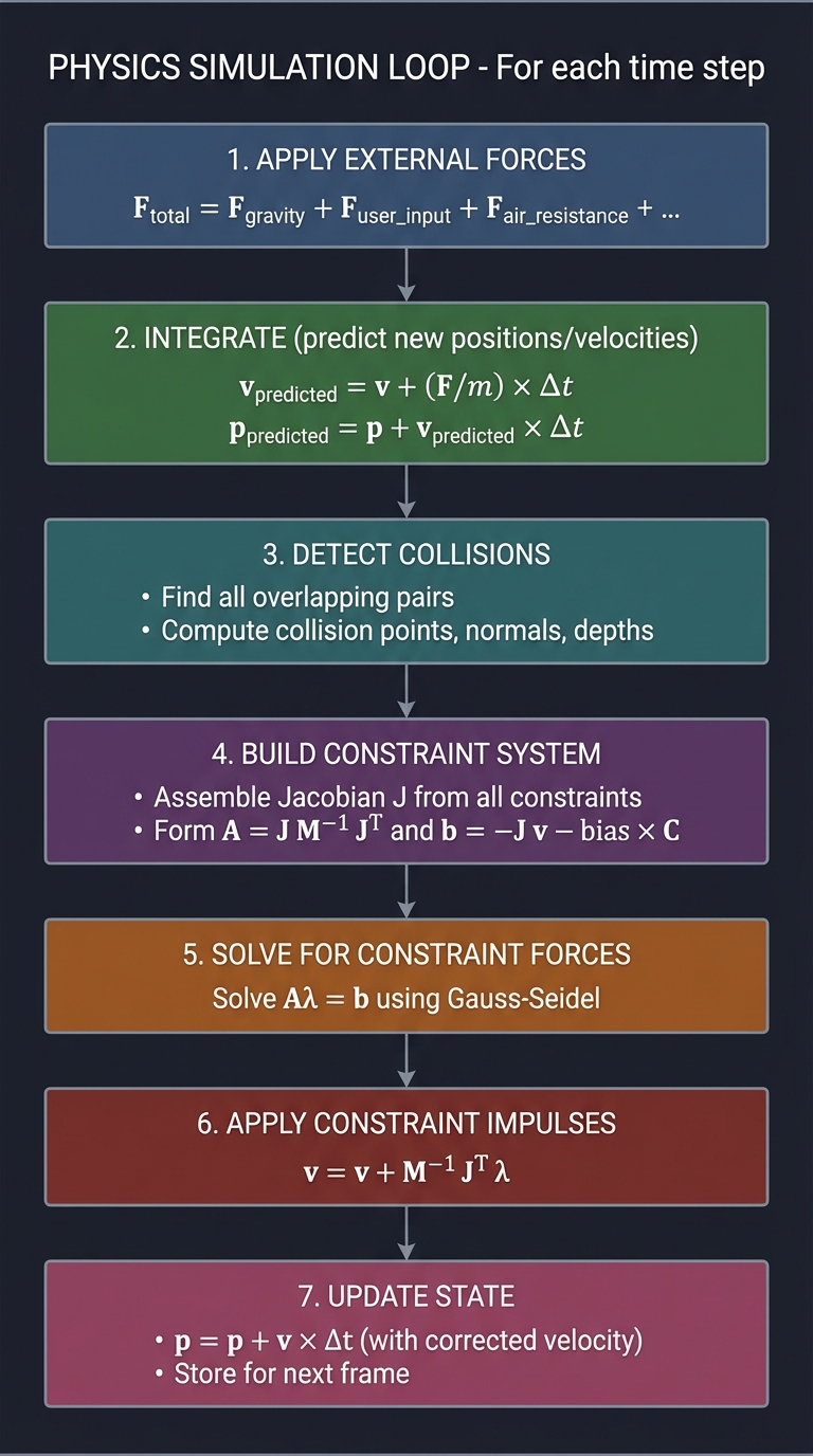
Part 9: Putting It Together - The Physics Loop
┌─────────────────────────────────────────────────────────────────────────┐
│                    PHYSICS SIMULATION LOOP                             │
├─────────────────────────────────────────────────────────────────────────┤
│                                                                         │
│  For each time step:                                                   │
│  ───────────────────                                                   │
│                                                                         │
│  ┌─────────────────────────────────────────────────────────────────┐   │
│  │ 1. APPLY EXTERNAL FORCES                                         │   │
│  │    F_total = F_gravity + F_user_input + F_air_resistance + ...   │   │
│  └──────────────────────────────────┬──────────────────────────────┘   │
│                                     │                                   │
│                                     ▼                                   │
│  ┌─────────────────────────────────────────────────────────────────┐   │
│  │ 2. INTEGRATE (predict new positions/velocities)                  │   │
│  │    v_predicted = v + (F/m) × Δt                                  │   │
│  │    p_predicted = p + v_predicted × Δt                            │   │
│  └──────────────────────────────────┬──────────────────────────────┘   │
│                                     │                                   │
│                                     ▼                                   │
│  ┌─────────────────────────────────────────────────────────────────┐   │
│  │ 3. DETECT COLLISIONS                                             │   │
│  │    Find all overlapping/intersecting pairs                       │   │
│  │    Compute collision points, normals, depths                     │   │
│  └──────────────────────────────────┬──────────────────────────────┘   │
│                                     │                                   │
│                                     ▼                                   │
│  ┌─────────────────────────────────────────────────────────────────┐   │
│  │ 4. BUILD CONSTRAINT SYSTEM                                       │   │
│  │    Assemble Jacobian J from all constraints                      │   │
│  │    Form A = J M⁻¹ Jᵀ  and  b = -J v - bias × C                  │   │
│  └──────────────────────────────────┬──────────────────────────────┘   │
│                                     │                                   │
│                                     ▼                                   │
│  ┌─────────────────────────────────────────────────────────────────┐   │
│  │ 5. SOLVE FOR CONSTRAINT FORCES                                   │   │
│  │    Solve A λ = b using Gauss-Seidel or PGS                       │   │
│  │    (possibly with warm starting from previous frame)             │   │
│  └──────────────────────────────────┬──────────────────────────────┘   │
│                                     │                                   │
│                                     ▼                                   │
│  ┌─────────────────────────────────────────────────────────────────┐   │
│  │ 6. APPLY CONSTRAINT IMPULSES                                     │   │
│  │    v = v + M⁻¹ Jᵀ λ                                              │   │
│  │    (constraints now satisfied)                                   │   │
│  └──────────────────────────────────┬──────────────────────────────┘   │
│                                     │                                   │
│                                     ▼                                   │
│  ┌─────────────────────────────────────────────────────────────────┐   │
│  │ 7. UPDATE STATE                                                  │   │
│  │    p = p + v × Δt  (with corrected velocity)                     │   │
│  │    Store for next frame                                          │   │
│  └─────────────────────────────────────────────────────────────────┘   │
│                                                                         │
└─────────────────────────────────────────────────────────────────────────┘
Project Specification
What You’re Building
A 2D physics simulator that:
- Simulates particles/circles under gravity
- Handles collisions with walls and other objects
- Supports spring/distance constraints
- Supports joint/pin constraints
- Renders in real-time
Minimum Requirements
- Particle system with gravity
- Semi-implicit Euler or Verlet integration
- Circle-circle collision detection and response
- Circle-wall collision (axis-aligned boundaries)
- Distance constraints (springs/rods)
- Simple constraint solver (Gauss-Seidel)
- Real-time rendering (SDL2 or similar)
Stretch Goals
- Rigid body rotation (not just particles)
- Friction in collisions
- Multiple joint types (hinges, sliders)
- Stacking and piles of objects
- Continuous collision detection
- Broad-phase acceleration (spatial hashing)
Solution Architecture
Data Structures
typedef struct {
    Vec2 position;
    Vec2 velocity;
    float mass;
    float inv_mass;  // 1/mass, or 0 for static objects
    float radius;
} Particle;

typedef struct {
    int particle_a;
    int particle_b;
    float rest_length;
    float stiffness;
} DistanceConstraint;

typedef struct {
    int particle_a;
    int particle_b;
    Vec2 normal;
    float penetration;
} Contact;

typedef struct {
    Particle* particles;
    int num_particles;
    DistanceConstraint* constraints;
    int num_constraints;
    Contact* contacts;
    int num_contacts;
    Vec2 gravity;
    float dt;
} PhysicsWorld;
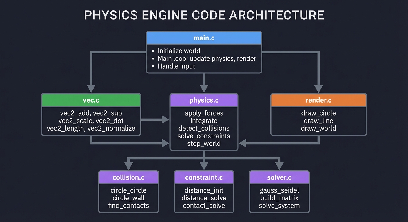
Module Structure
┌─────────────────────────────────────────────────────────────────┐
│                           main.c                                │
│  - Initialize world                                             │
│  - Main loop: update physics, render                           │
│  - Handle input                                                 │
└─────────────────────────────────────────────────────────────────┘
                               │
        ┌──────────────────────┼──────────────────────┐
        ▼                      ▼                      ▼
┌──────────────┐      ┌──────────────┐      ┌──────────────┐
│   vec.c      │      │  physics.c   │      │  render.c    │
│              │      │              │      │              │
│ vec2_add     │      │ apply_forces │      │ draw_circle  │
│ vec2_sub     │      │ integrate    │      │ draw_line    │
│ vec2_scale   │      │ detect_collisions │ │ draw_world   │
│ vec2_dot     │      │ solve_constraints  │ │              │
│ vec2_length  │      │ step_world   │      │              │
│ vec2_normalize│     │              │      │              │
└──────────────┘      └──────────────┘      └──────────────┘
                               │
        ┌──────────────────────┼──────────────────────┐
        ▼                      ▼                      ▼
┌──────────────┐      ┌──────────────┐      ┌──────────────┐
│  collision.c │      │  constraint.c│      │  solver.c    │
│              │      │              │      │              │
│ circle_circle│      │ distance_init│      │ gauss_seidel │
│ circle_wall  │      │ distance_solve│     │ build_matrix │
│ find_contacts│      │ contact_solve│      │ solve_system │
└──────────────┘      └──────────────┘      └──────────────┘
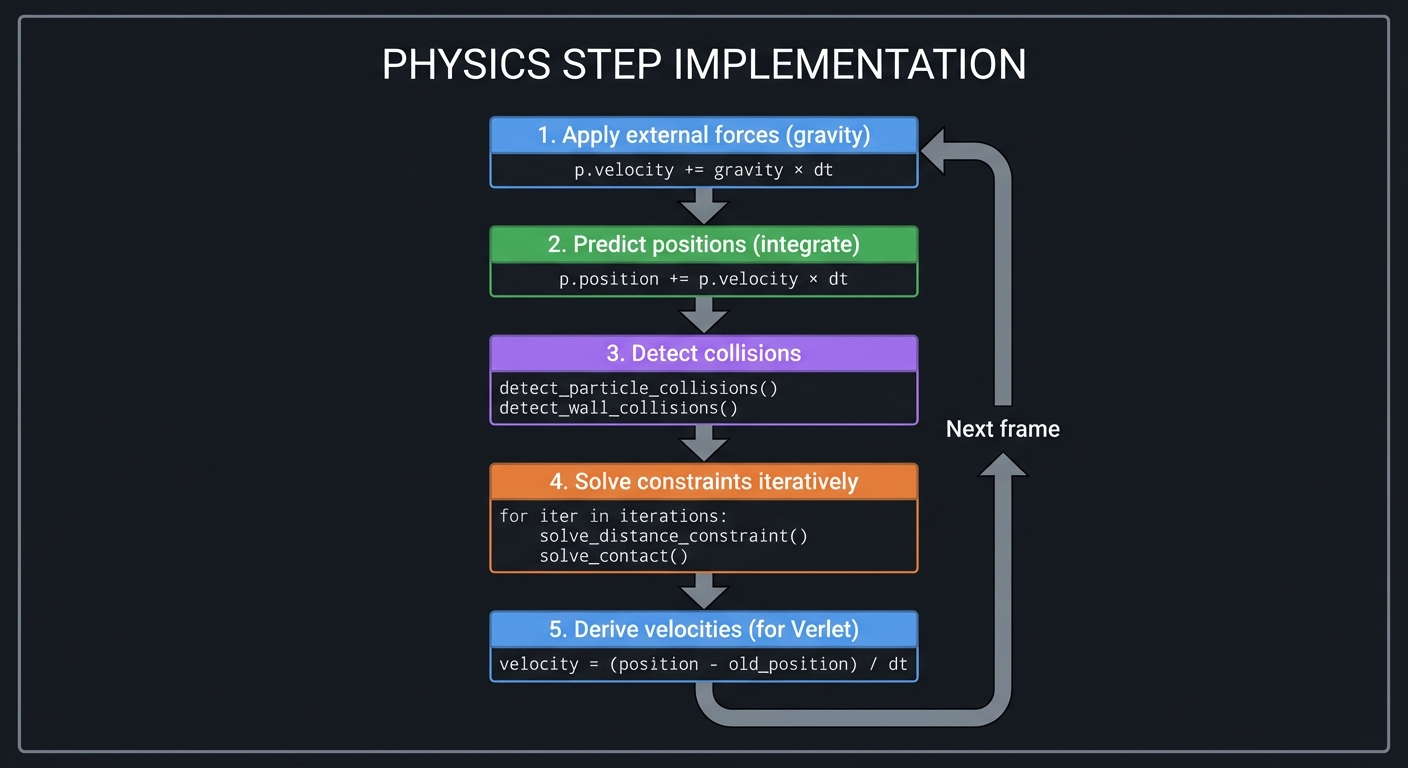
Simulation Loop Flow
┌─────────────────────────────────────────────────────────────────────────┐
│                      PHYSICS STEP IMPLEMENTATION                       │
├─────────────────────────────────────────────────────────────────────────┤
│                                                                         │
│  void physics_step(PhysicsWorld* world) {                              │
│                                                                         │
│      // 1. Apply external forces (gravity)                             │
│      for each particle p:                                              │
│          p.velocity += world.gravity * world.dt                        │
│                                                                         │
│      // 2. Predict positions (integrate)                               │
│      for each particle p:                                              │
│          p.position += p.velocity * world.dt                           │
│                                                                         │
│      // 3. Detect collisions                                           │
│      world.num_contacts = 0                                            │
│      detect_particle_collisions(world)                                 │
│      detect_wall_collisions(world)                                     │
│                                                                         │
│      // 4. Solve constraints iteratively                               │
│      for (int iter = 0; iter < NUM_ITERATIONS; iter++) {               │
│          // Solve distance constraints                                 │
│          for each constraint c:                                        │
│              solve_distance_constraint(c, world.particles)             │
│                                                                         │
│          // Solve contact constraints                                  │
│          for each contact c:                                           │
│              solve_contact(c, world.particles)                         │
│      }                                                                  │
│                                                                         │
│      // 5. Derive velocities from position changes (for Verlet)        │
│      for each particle p:                                              │
│          p.velocity = (p.position - p.old_position) / world.dt        │
│  }                                                                      │
│                                                                         │
└─────────────────────────────────────────────────────────────────────────┘
Phased Implementation Guide
Phase 1: Basic Particle Simulation (Days 1-4)
Goal: Particles falling under gravity
Tasks:
- Implement Vec2 math library
- Create Particle structure
- Implement semi-implicit Euler integration
- Add gravity
- Render particles with SDL2
Implementation:
void integrate_particles(PhysicsWorld* world) {
    float dt = world->dt;
    for (int i = 0; i < world->num_particles; i++) {
        Particle* p = &world->particles[i];
        // Apply gravity
        p->velocity = vec2_add(p->velocity, vec2_scale(world->gravity, dt));
        // Update position
        p->position = vec2_add(p->position, vec2_scale(p->velocity, dt));
    }
}
Verification:
- Particles should fall downward
- Velocity should increase over time
- Position change should match v × Δt
Phase 2: Wall Collisions (Days 5-7)
Goal: Particles bounce off screen boundaries
Tasks:
- Detect when particle exits bounds
- Compute collision normal
- Implement reflection formula
- Add coefficient of restitution
Implementation:
void collide_with_walls(Particle* p, float width, float height, float restitution) {
    // Left wall
    if (p->position.x - p->radius < 0) {
        p->position.x = p->radius;
        p->velocity.x = -p->velocity.x * restitution;
    }
    // Right wall
    if (p->position.x + p->radius > width) {
        p->position.x = width - p->radius;
        p->velocity.x = -p->velocity.x * restitution;
    }
    // Similarly for top/bottom
}
Verification:
- Particles bounce off walls
- Restitution = 1: energy conserved
- Restitution = 0.5: each bounce loses energy
Phase 3: Particle-Particle Collisions (Days 8-11)
Goal: Particles collide with each other
Tasks:
- Detect circle-circle overlap
- Compute collision normal and penetration
- Implement impulse-based response
- Handle position correction
Implementation:
void detect_circle_collision(Particle* a, Particle* b, Contact* contact) {
    Vec2 delta = vec2_sub(b->position, a->position);
    float dist = vec2_length(delta);
    float min_dist = a->radius + b->radius;

    if (dist < min_dist) {
        contact->normal = vec2_scale(delta, 1.0f / dist);
        contact->penetration = min_dist - dist;
        contact->valid = true;
    } else {
        contact->valid = false;
    }
}

void resolve_collision(Particle* a, Particle* b, Contact* c, float restitution) {
    Vec2 rel_vel = vec2_sub(a->velocity, b->velocity);
    float vel_along_normal = vec2_dot(rel_vel, c->normal);

    // Don't resolve if separating
    if (vel_along_normal > 0) return;

    // Compute impulse
    float j = -(1 + restitution) * vel_along_normal;
    j /= a->inv_mass + b->inv_mass;

    Vec2 impulse = vec2_scale(c->normal, j);
    a->velocity = vec2_add(a->velocity, vec2_scale(impulse, a->inv_mass));
    b->velocity = vec2_sub(b->velocity, vec2_scale(impulse, b->inv_mass));

    // Position correction (prevent sinking)
    float correction = c->penetration / (a->inv_mass + b->inv_mass) * 0.8f;
    a->position = vec2_sub(a->position, vec2_scale(c->normal, a->inv_mass * correction));
    b->position = vec2_add(b->position, vec2_scale(c->normal, b->inv_mass * correction));
}
Verification:
- Particles bounce off each other
- Momentum is conserved
- No permanent interpenetration
Phase 4: Distance Constraints (Days 12-15)
Goal: Connect particles with springs/rods
Tasks:
- Define distance constraint structure
- Compute constraint violation
- Implement iterative position correction
- Visualize constraints
Implementation:
void solve_distance_constraint(DistanceConstraint* c, Particle* particles) {
    Particle* a = &particles[c->particle_a];
    Particle* b = &particles[c->particle_b];

    Vec2 delta = vec2_sub(b->position, a->position);
    float current_length = vec2_length(delta);
    float error = current_length - c->rest_length;

    if (current_length < 0.0001f) return;  // Avoid division by zero

    // Correction direction
    Vec2 correction = vec2_scale(delta, error / current_length);

    // Apply correction based on inverse masses
    float total_inv_mass = a->inv_mass + b->inv_mass;
    if (total_inv_mass < 0.0001f) return;  // Both static

    a->position = vec2_add(a->position, vec2_scale(correction, a->inv_mass / total_inv_mass));
    b->position = vec2_sub(b->position, vec2_scale(correction, b->inv_mass / total_inv_mass));
}
Verification:
- Connected particles maintain distance
- Multiple iterations improve constraint satisfaction
- Chain of particles behaves like rope
Phase 5: Building the Constraint Solver (Days 16-19)
Goal: Unified constraint solving system
Tasks:
- Abstract constraint interface
- Build constraint Jacobian
- Implement Gauss-Seidel solver
- Handle mixed constraint types
Implementation:
// Generic constraint solver (simplified)
void solve_constraints(PhysicsWorld* world, int iterations) {
    for (int iter = 0; iter < iterations; iter++) {
        // Distance constraints
        for (int i = 0; i < world->num_constraints; i++) {
            solve_distance_constraint(&world->constraints[i], world->particles);
        }

        // Contact constraints
        for (int i = 0; i < world->num_contacts; i++) {
            solve_contact(&world->contacts[i], world->particles);
        }
    }
}
Verification:
- All constraints satisfied (within tolerance)
- Stable with many constraints
- Convergence improves with iterations
Phase 6: Complex Scenes (Days 20-23)
Goal: Build interesting simulations
Tasks:
- Create chain/rope scene
- Create bridge scene
- Create cloth-like grid
- Add user interaction (drag, spawn)
Scenes to implement:
void create_rope_scene(PhysicsWorld* world) {
    // Chain of particles with distance constraints
    for (int i = 0; i < 10; i++) {
        add_particle(world, i * 30, 100, 5);
        if (i > 0) {
            add_distance_constraint(world, i-1, i, 30);
        }
    }
    // Pin first particle
    world->particles[0].inv_mass = 0;  // Static
}

void create_soft_body_scene(PhysicsWorld* world) {
    // Grid of particles with structural and shear constraints
    int grid_size = 5;
    for (int y = 0; y < grid_size; y++) {
        for (int x = 0; x < grid_size; x++) {
            add_particle(world, 200 + x * 30, 100 + y * 30, 5);
        }
    }
    // Add constraints (structural, shear, bend)
    // ...
}
Verification:
- Rope swings realistically
- Soft body maintains shape but deforms
- No explosions or jitter
Phase 7: Polish and Optimization (Days 24-28)
Goal: Make it robust and fast
Tasks:
- Add friction to collisions
- Implement warm starting
- Add broad-phase collision detection
- Profile and optimize
Friction:
void apply_friction(Particle* a, Particle* b, Contact* c, float friction) {
    Vec2 rel_vel = vec2_sub(a->velocity, b->velocity);
    Vec2 tangent = vec2_sub(rel_vel, vec2_scale(c->normal, vec2_dot(rel_vel, c->normal)));
    float tangent_speed = vec2_length(tangent);

    if (tangent_speed < 0.001f) return;

    tangent = vec2_scale(tangent, 1.0f / tangent_speed);
    float jt = -vec2_dot(rel_vel, tangent) / (a->inv_mass + b->inv_mass);

    // Clamp to Coulomb friction
    jt = clamp(jt, -friction * c->normal_impulse, friction * c->normal_impulse);

    Vec2 friction_impulse = vec2_scale(tangent, jt);
    a->velocity = vec2_add(a->velocity, vec2_scale(friction_impulse, a->inv_mass));
    b->velocity = vec2_sub(b->velocity, vec2_scale(friction_impulse, b->inv_mass));
}
Verification:
- Objects stack without sliding
- System remains stable under stress
- 60 FPS with 100+ objects
Testing Strategy
Unit Tests
- Vector operations:
- Dot product of perpendicular vectors = 0
- Normalized vector has length 1
- Reflection formula is correct
- Collision detection:
- Overlapping circles detected
- Non-overlapping circles not detected
- Normal points from A to B
- Integration:
- Constant velocity → position increases linearly
- Constant acceleration → velocity increases linearly
- Constraints:
- Distance constraint maintains length
- Constraint solver converges
Physical Validation
- Conservation of energy (elastic collision, no gravity)
- Conservation of momentum (any collision)
- Projectile motion (matches v₀t + ½gt²)
- Pendulum period (matches 2π√(L/g))
Stress Tests
- Many particles: 100+ without slowdown
- Long chains: 50+ links stable
- Stacking: 10+ objects stable
- High speeds: No tunneling through walls
Common Pitfalls and Debugging
Explosion/Instability
Symptom: Particles fly off to infinity
Causes:
- Time step too large
- Forces computed incorrectly
- Penetration not resolved
Fixes:
- Reduce Δt (try 1/120 instead of 1/60)
- Add position correction
- Clamp velocities to maximum
Sinking Objects
Symptom: Objects slowly fall through floors
Causes:
- Collision detected but not resolved
- Bias/slop too large
- Not enough solver iterations
Fixes:
- Add position correction after velocity correction
- Reduce bias (e.g., 0.01 instead of 0.1)
- Increase iterations (10-20)
Jitter/Vibration
Symptom: Objects vibrate in place
Causes:
- Over-correction
- Conflicting constraints
- No damping
Fixes:
- Add damping: v *= 0.99
- Reduce correction factor
- Warm start solver
Constraint Stretching
Symptom: Springs stretch too much
Causes:
- Not enough solver iterations
- Stiffness too low
- Integration error
Fixes:
- More iterations (20+)
- Use position-based dynamics
- Smaller time step
Tunneling
Symptom: Fast objects pass through walls
Causes:
- Discrete collision detection
- Large time step
- Small obstacles
Fixes:
- Continuous collision detection (CCD)
- Limit max velocity
- Sub-step physics
Extensions and Challenges
Beginner Extensions
- Add mouse interaction (drag particles)
- Create preset scenes (bridge, rope, dominos)
- Add visual effects (trails, colors)
Intermediate Extensions
- Implement friction
- Add rigid body rotation
- Create hinge joints
- Implement spatial hashing for broad phase
Advanced Extensions
- Continuous collision detection
- 3D extension
- Deformable bodies
- Fluid simulation (SPH)
Real-World Connections
Game Engines
Every physics engine (Box2D, Bullet, PhysX) uses these concepts:
- Constraint-based dynamics
- Iterative solvers
- Warm starting
- Continuous collision detection
Robotics
Robot dynamics and control:
- Forward/inverse kinematics
- Constraint satisfaction
- Force/torque computation
Computer Graphics
Physically-based animation:
- Cloth simulation
- Hair dynamics
- Destruction effects
Engineering Simulation
Structural analysis:
- Finite element methods
- Stress/strain computation
- Dynamic loading
Self-Assessment Checklist
Conceptual Understanding
- I can explain why we need to solve Ax = b for physics
- I understand the role of the Jacobian matrix
- I can describe why iterative solvers work for constraints
- I know what matrix conditioning means for stability
- I understand the tradeoffs of different integration methods
Practical Skills
- I implemented collision detection and response
- I built a working constraint solver
- My simulation runs stable at 60 FPS
- I can create various constraint types
- I can debug common physics bugs
Teaching Test
Can you explain to someone else:
- How does impulse-based collision response work?
- Why do constraints create systems of equations?
- What makes a simulation stable vs. unstable?
- How does Gauss-Seidel iteration work?
Resources
Primary
- “Game Physics Engine Development” by Ian Millington
- “Physics for Game Developers” by David Bourg
- Box2D source code - Reference implementation
Reference
- “Real-Time Collision Detection” by Christer Ericson
- “Numerical Recipes in C” by Press et al. - Equation solvers
- Erin Catto’s GDC presentations - Box2D author’s talks
Online
- Box2D documentation - Algorithm explanations
- Gaffer On Games (gafferongames.com) - Physics articles
- Two-Bit Coding YouTube - Physics engine tutorials
When you complete this project, you’ll understand that physics simulation is applied linear algebra—solving equations, projecting vectors, and navigating numerical challenges. Every game, every simulation, every robot uses these techniques.