P03: Neural Network from Scratch
Build a neural network that classifies handwritten digits, implementing forward propagation, backpropagation, and training—using only matrix operations.
Overview
| Attribute | Value |
|---|---|
| Difficulty | Intermediate-Advanced |
| Time Estimate | 2-3 weeks |
| Language | Python (recommended) or C |
| Prerequisites | Calculus basics (derivatives), matrix multiplication |
| Primary Book | “Math for Programmers” by Paul Orland |
Learning Objectives
By completing this project, you will:
- See neural networks as linear algebra - Every layer is matrix multiplication + nonlinearity
- Master the chain rule in matrix form - Backpropagation is gradient computation
- Understand gradient descent geometrically - Navigating high-dimensional landscapes
- Grasp matrix transposes deeply - Why they appear in backprop
- Internalize batch processing - Matrix-matrix multiplication for efficiency
- Connect math to learning - Watch abstract matrices develop “knowledge”
Theoretical Foundation
Part 1: The Neuron - A Linear Function Plus Nonlinearity
A Single Neuron
The fundamental building block:
┌────────────────────────────────────────────────────────────────┐
│                      SINGLE NEURON                             │
├────────────────────────────────────────────────────────────────┤
│                                                                │
│    Inputs              Weights          Sum          Output    │
│                                                                │
│    x₁ ───────w₁────┐                                          │
│                     │                                          │
│    x₂ ───────w₂────┼────→ Σ(wᵢxᵢ) + b ──→ σ(z) ──→ a         │
│                     │           ↑                              │
│    x₃ ───────w₃────┘           │                              │
│                               bias                             │
│                                                                │
│    Linear part:     z = w₁x₁ + w₂x₂ + w₃x₃ + b               │
│    Activation:      a = σ(z)                                  │
│                                                                │
└────────────────────────────────────────────────────────────────┘
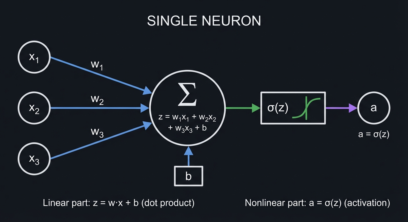
The linear part (z):
z = w · x + b = w₁x₁ + w₂x₂ + ... + wₙxₙ + b

This is a dot product! It measures how much the input aligns
with the weight vector.
The nonlinear part (activation function σ):
- Without nonlinearity, stacking layers would still be linear
- Common activations: sigmoid, tanh, ReLU
Why Nonlinearity is Essential
Linear layer 1:  y = W₁x + b₁
Linear layer 2:  z = W₂y + b₂ = W₂(W₁x + b₁) + b₂ = W₂W₁x + (W₂b₁ + b₂)

This is still just z = Ax + c — a single linear transformation!
Stacking linear layers gains nothing.

With nonlinearity:  y = σ(W₁x + b₁)
                    z = σ(W₂y + b₂)

Now the composition is nonlinear — can approximate any function!
Part 2: The Layer - Many Neurons in Parallel
From Neuron to Layer
Instead of one neuron, we compute many simultaneously:
┌────────────────────────────────────────────────────────────────┐
│                      NEURAL NETWORK LAYER                      │
├────────────────────────────────────────────────────────────────┤
│                                                                │
│    Input         Weight Matrix         Bias      Activation   │
│    Vector                              Vector                  │
│                                                                │
│    [x₁]     [w₁₁  w₁₂  w₁₃]   [x₁]     [b₁]                   │
│    [x₂]  →  [w₂₁  w₂₂  w₂₃] × [x₂]  +  [b₂]  →  σ()  →  [a₁] │
│    [x₃]     [w₃₁  w₃₂  w₃₃]   [x₃]     [b₃]           [a₂] │
│             [w₄₁  w₄₂  w₄₃]            [b₄]           [a₃] │
│                                                        [a₄] │
│                                                                │
│    3 inputs → 4 outputs (4 neurons)                           │
│    Weight matrix: 4×3 (rows = neurons, columns = inputs)      │
│                                                                │
└────────────────────────────────────────────────────────────────┘
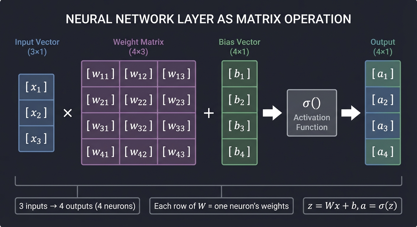
The matrix equation:
z = Wx + b
a = σ(z)

Where:
- x is the input vector (n×1)
- W is the weight matrix (m×n)
- b is the bias vector (m×1)
- z is the pre-activation (m×1)
- a is the output/activation (m×1)
Each row of W is one neuron’s weight vector:
Row 1 of W = weights for neuron 1
Row 2 of W = weights for neuron 2
...

(Wx)ᵢ = row i of W · x = weighted sum for neuron i
Part 3: The Network - Layers Composed
Multi-Layer Architecture
┌─────────────────────────────────────────────────────────────────────────┐
│                    MULTI-LAYER NEURAL NETWORK                          │
├─────────────────────────────────────────────────────────────────────────┤
│                                                                         │
│    Input        Hidden Layer 1      Hidden Layer 2       Output        │
│    (784)            (128)               (64)             (10)          │
│                                                                         │
│     x               a¹                  a²                 ŷ           │
│    [·]             [·]                 [·]               [·]           │
│    [·]    W¹,b¹    [·]      W²,b²     [·]     W³,b³     [·]           │
│    [·]   ────────→ [·]    ────────→   [·]   ────────→   [·]           │
│    [·]     σ       [·]       σ        [·]      σ        [·]           │
│    ...             ...                 ...               ...           │
│    [·]             [·]                 [·]               [·]           │
│                                                                         │
│    For MNIST:                                                          │
│    - Input: 28×28 = 784 pixels                                         │
│    - Output: 10 classes (digits 0-9)                                   │
│    - Hidden layers: learn intermediate features                        │
│                                                                         │
└─────────────────────────────────────────────────────────────────────────┘
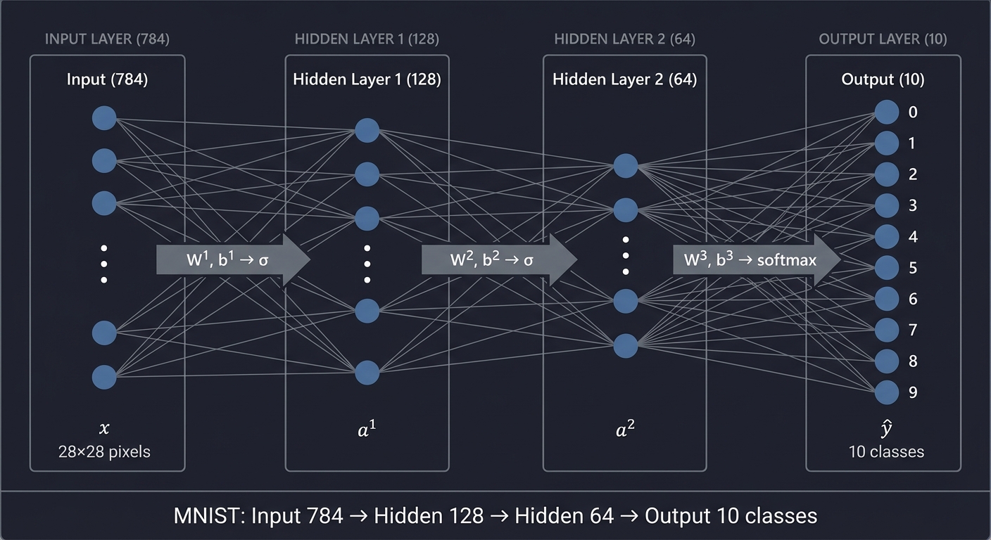
Forward propagation equations:
Layer 1:  z¹ = W¹x + b¹,     a¹ = σ(z¹)
Layer 2:  z² = W²a¹ + b²,    a² = σ(z²)
Layer 3:  z³ = W³a² + b³,    ŷ = softmax(z³)
Dimensions for MNIST:
Input x:    784 × 1
W¹:         128 × 784     a¹: 128 × 1
W²:         64 × 128      a²: 64 × 1
W³:         10 × 64       ŷ:  10 × 1

Total parameters: 128×784 + 128 + 64×128 + 64 + 10×64 + 10 = 109,386
Part 4: Activation Functions
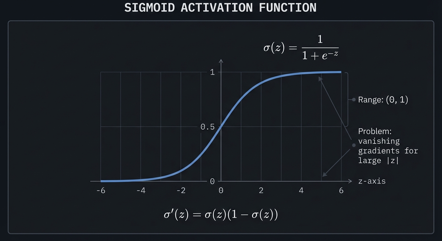
Sigmoid
σ(z) = 1 / (1 + e⁻ᶻ)

Range: (0, 1)
Derivative: σ'(z) = σ(z)(1 - σ(z))

Graph:
    1 ──────────────═══════════
      │           ╱
      │         ╱
    0.5 ───────●───────────────
      │       ╱│
      │     ╱  │
    0 ═════════┴───────────────
              0       z

Problem: "vanishing gradients" — derivative → 0 for large |z|
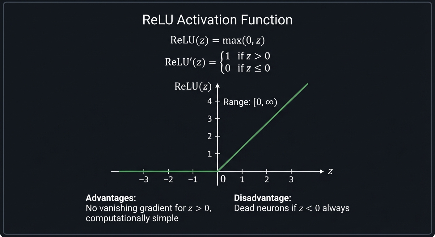
ReLU (Rectified Linear Unit)
ReLU(z) = max(0, z)

Range: [0, ∞)
Derivative: 1 if z > 0, else 0

Graph:
    │      ╱
    │    ╱
    │  ╱
    │╱
    ●─────────────
   0              z

Advantages: No vanishing gradient (for z > 0), computationally simple
Disadvantage: "Dead neurons" if z < 0 always
Softmax (for output layer classification)
softmax(zᵢ) = e^zᵢ / Σⱼ e^zⱼ

Converts raw scores to probabilities:
- All outputs sum to 1
- Each output ∈ (0, 1)

Example:
z = [2.0, 1.0, 0.1]
e^z = [7.39, 2.72, 1.11]
softmax(z) = [0.66, 0.24, 0.10]  ← probabilities for 3 classes
Part 5: The Loss Function
Cross-Entropy Loss
For classification, we use cross-entropy:
L = -Σᵢ yᵢ log(ŷᵢ)

Where:
- y is the true label (one-hot encoded)
- ŷ is the predicted probability

For single correct class c:
L = -log(ŷc)

If we predict high probability for correct class: L is small
If we predict low probability for correct class: L is large
Example:
True label: 3 (one-hot: [0,0,0,1,0,0,0,0,0,0])
Prediction: [0.01, 0.01, 0.02, 0.90, 0.02, 0.01, 0.01, 0.01, 0.005, 0.005]

L = -log(0.90) ≈ 0.105  (good prediction, low loss)

Bad prediction: [0.1, 0.1, 0.1, 0.1, 0.1, 0.1, 0.1, 0.1, 0.1, 0.1]
L = -log(0.1) ≈ 2.303   (poor prediction, high loss)
Part 6: Gradient Descent
The Optimization Problem
Find weights W*, b* that minimize:

L(W, b) = (1/N) Σᵢ Loss(network(xᵢ; W, b), yᵢ)

Where the sum is over all training examples.
The Gradient Descent Update
W := W - α × ∂L/∂W
b := b - α × ∂L/∂b
Where α is the learning rate.
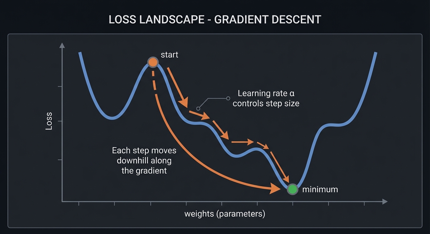
Intuition: Move in the direction of steepest descent.
Geometric picture:
┌────────────────────────────────────────────────────────────────┐
│                   LOSS LANDSCAPE                               │
├────────────────────────────────────────────────────────────────┤
│                                                                │
│    Loss                                                        │
│     │      ╱╲                                                  │
│     │     ╱  ╲    ╱╲                                           │
│     │    ╱    ╲  ╱  ╲                                          │
│     │   ╱      ╲╱    ╲____╱╲                                   │
│     │  ╱                    ╲___                               │
│     │ ●─→─→─→─→─→─→─→─→─→─→─→─→●  (minimum)                   │
│     └──────────────────────────────────── weights              │
│                                                                │
│   Each step moves downhill along the gradient.                 │
│   Learning rate α controls step size.                          │
│                                                                │
└────────────────────────────────────────────────────────────────┘
Stochastic Gradient Descent (SGD)
Instead of computing gradient over all examples:
For each mini-batch of size B:
    1. Forward pass: compute predictions
    2. Compute loss
    3. Backward pass: compute gradients
    4. Update weights
Advantages:
- Faster iterations
- Noise helps escape local minima
- Fits in memory
Part 7: Backpropagation - The Chain Rule in Matrices
The Chain Rule Review
For scalar functions:
If y = f(g(x)), then dy/dx = (dy/dg) × (dg/dx)
For matrices, we need to track shapes carefully.
Backward Through One Layer
Consider layer: a = σ(Wx + b)
We receive from the next layer: ∂L/∂a (gradient w.r.t. this layer’s output)
We need to compute:
∂L/∂W = ?
∂L/∂b = ?
∂L/∂x = ? (to pass to previous layer)
Step 1: Gradient through activation
∂L/∂z = ∂L/∂a ⊙ σ'(z)

Where ⊙ is element-wise multiplication.
Each element of z affects its corresponding element of a.
Step 2: Gradient w.r.t. weights
z = Wx + b
∂z/∂W = ?

The key insight: zᵢ = Σⱼ Wᵢⱼ xⱼ
So ∂zᵢ/∂Wᵢⱼ = xⱼ

In matrix form: ∂L/∂W = (∂L/∂z) × xᵀ
                         (m×1)   (1×n)  =  (m×n)

This is an outer product!
Step 3: Gradient w.r.t. bias
∂L/∂b = ∂L/∂z

(bias adds directly to z, so gradient passes through)
Step 4: Gradient w.r.t. input (to pass backward)
z = Wx + b
∂zᵢ/∂xⱼ = Wᵢⱼ

In matrix form: ∂L/∂x = Wᵀ × (∂L/∂z)
                        (n×m)  (m×1)  =  (n×1)

THE TRANSPOSE APPEARS! This is why understanding transposes matters.
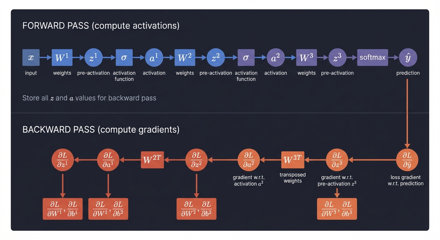
The Full Backpropagation Algorithm
┌─────────────────────────────────────────────────────────────────────────┐
│                    BACKPROPAGATION FLOW                                │
├─────────────────────────────────────────────────────────────────────────┤
│                                                                         │
│  FORWARD PASS (compute activations)                                    │
│  ─────────────────────────────────                                     │
│  x ──W¹──→ z¹ ──σ──→ a¹ ──W²──→ z² ──σ──→ a² ──W³──→ z³ ──softmax──→ ŷ│
│                                                                         │
│  Store all z's and a's — needed for backward pass!                     │
│                                                                         │
│  BACKWARD PASS (compute gradients)                                     │
│  ──────────────────────────────────                                    │
│  ∂L/∂ŷ ←── ∂L/∂z³ ←─W³ᵀ── ∂L/∂a² ←── ∂L/∂z² ←─W²ᵀ── ∂L/∂a¹ ←── ∂L/∂z¹│
│               │               │               │               │        │
│               ▼               ▼               ▼               ▼        │
│            ∂L/∂W³          ∂L/∂W²          ∂L/∂W¹          (done)      │
│            ∂L/∂b³          ∂L/∂b²          ∂L/∂b¹                      │
│                                                                         │
└─────────────────────────────────────────────────────────────────────────┘
Pseudocode:
def backward(self, dL_dy):
    # For each layer, from last to first:
    for layer in reversed(self.layers):
        # Gradient through activation
        dL_dz = dL_dy * activation_derivative(layer.z)

        # Gradients for this layer's parameters
        layer.dW = outer(dL_dz, layer.input)
        layer.db = dL_dz

        # Gradient to pass to previous layer
        dL_dy = layer.W.T @ dL_dz

    return  # Gradients stored in each layer
Part 8: Batch Processing with Matrices
Single Example vs. Batch
Single example:
x: (n, 1) vector
z = Wx + b
a = σ(z)
Batch of B examples:
X: (n, B) matrix — each column is one example
Z = WX + b (broadcast b to each column)
A = σ(Z)
Why batches?:
- GPU parallelism: matrix-matrix multiplication is optimized
- Gradient averaging: smoother optimization
- Memory efficiency: process in chunks
Matrix dimensions for batch:
X:     (784, 32)  — 32 images, each 784 pixels
W¹:    (128, 784)
Z¹:    (128, 32)  — 32 outputs, each with 128 neurons
A¹:    (128, 32)
...
Ŷ:     (10, 32)   — 32 predictions, each with 10 classes
Backprop with Batches
The gradients need to be summed (or averaged) over the batch:
# Forward
Z = W @ X + b.reshape(-1, 1)  # broadcast bias
A = activation(Z)

# Backward
dL_dZ = dL_dA * activation_derivative(Z)
dL_dW = (dL_dZ @ X.T) / batch_size  # average over batch
dL_db = dL_dZ.mean(axis=1)          # average over batch
dL_dX = W.T @ dL_dZ
Part 9: Weight Initialization
Why Initialization Matters
Bad initialization → gradients vanish or explode → training fails
Problem: If weights are too large, activations saturate (sigmoid → 0 or 1)
         If weights are too small, activations collapse to zero

The variance of activations should stay roughly constant through layers.
Xavier/Glorot Initialization
For sigmoid/tanh:
W ~ Normal(0, sqrt(2 / (fan_in + fan_out)))

Or equivalently:
W ~ Uniform(-sqrt(6 / (fan_in + fan_out)), sqrt(6 / (fan_in + fan_out)))

Where:
- fan_in = number of input neurons
- fan_out = number of output neurons
He Initialization
For ReLU:
W ~ Normal(0, sqrt(2 / fan_in))
The math: ReLU zeros out half the activations, so we need 2× variance to compensate.
Part 10: Understanding Through Linear Algebra
Neural Networks as Function Composition
f(x) = σL(WL × σL₋₁(WL₋₁ × ... σ₁(W₁ × x + b₁) ... + bL₋₁) + bL)

Each layer:
1. Linearly transforms (rotates, scales, translates via W and b)
2. Applies pointwise nonlinearity (σ)

The sequence of transformations warps the input space to make
classification easier.
What Each Layer “Sees”
Layer 1: Raw pixels
Layer 2: Edges and simple patterns (combinations of pixels)
Layer 3: Shapes and parts (combinations of edges)
Layer 4: Objects and digits (combinations of shapes)
Output:  Class probabilities
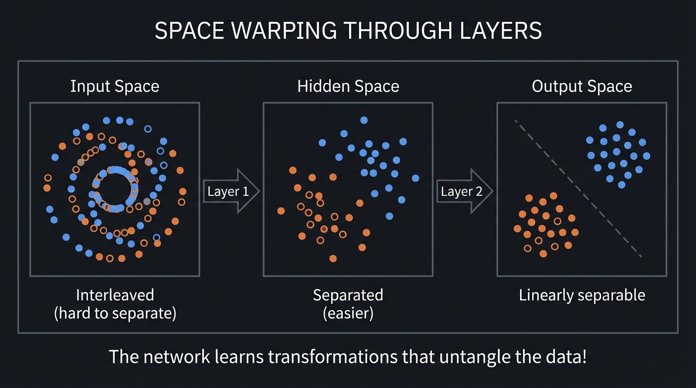
The Geometry of Classification
┌────────────────────────────────────────────────────────────────┐
│             SPACE WARPING THROUGH LAYERS                       │
├────────────────────────────────────────────────────────────────┤
│                                                                │
│    Input Space          Hidden Space         Output Space      │
│                                                                │
│    ● ● ●                    ●                     ●            │
│    ○ ○ ○    Layer 1     ○       ○   Layer 2                    │
│    ● ● ●   ────────→        ●      ────────→   ○              │
│    ○ ○ ○                ○       ○                              │
│                            ●                     ●             │
│                                                                │
│   Interleaved           Separated              Linearly        │
│   (hard to separate)    (easier)               separable       │
│                                                                │
│   The network learns transformations that untangle the data!   │
│                                                                │
└────────────────────────────────────────────────────────────────┘
Project Specification
What You’re Building
A neural network that:
- Loads the MNIST dataset (handwritten digits)
- Implements forward propagation with matrix operations
- Implements backpropagation to compute gradients
- Trains using stochastic gradient descent
- Achieves >95% accuracy on test set
Minimum Requirements
- Load and preprocess MNIST data
- Implement matrix operations (or use numpy)
- Build network with at least 2 hidden layers
- Implement ReLU and softmax activations
- Implement cross-entropy loss
- Implement backpropagation from scratch
- Train and achieve >95% test accuracy
- Plot training loss over epochs
Stretch Goals
- Implement multiple optimizers (SGD, momentum, Adam)
- Add dropout regularization
- Visualize learned weights as images
- Implement convolutional layers
- Add batch normalization
Solution Architecture
Data Structures
class Layer:
    """A single neural network layer."""

    def __init__(self, input_size: int, output_size: int, activation: str):
        self.W = initialize_weights(input_size, output_size)
        self.b = np.zeros((output_size, 1))
        self.activation = activation

        # Stored during forward pass for backprop
        self.input = None
        self.z = None
        self.a = None

        # Gradients computed during backward pass
        self.dW = None
        self.db = None

class NeuralNetwork:
    """Multi-layer neural network."""

    def __init__(self, layer_sizes: list, activations: list):
        self.layers = []
        for i in range(len(layer_sizes) - 1):
            self.layers.append(Layer(
                layer_sizes[i],
                layer_sizes[i + 1],
                activations[i]
            ))

    def forward(self, X: np.ndarray) -> np.ndarray:
        """Compute forward pass, return output."""
        pass

    def backward(self, Y: np.ndarray) -> None:
        """Compute gradients via backpropagation."""
        pass

    def update(self, learning_rate: float) -> None:
        """Apply gradient descent update."""
        pass
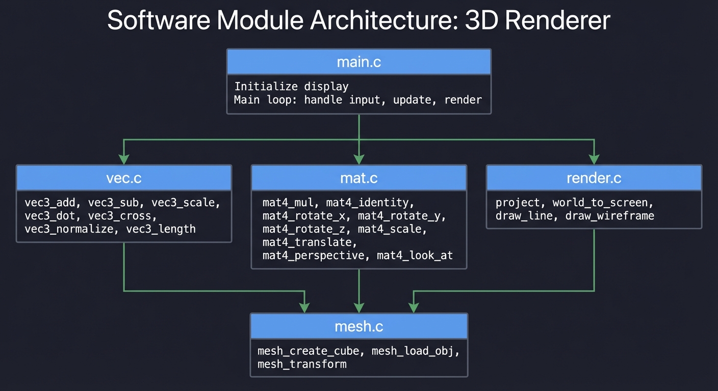
Module Structure
┌─────────────────────────────────────────────────────────────────┐
│                           main.py                               │
│  - Load MNIST                                                   │
│  - Training loop                                                │
│  - Evaluation and visualization                                 │
└─────────────────────────────────────────────────────────────────┘
                               │
        ┌──────────────────────┼──────────────────────┐
        ▼                      ▼                      ▼
┌──────────────┐      ┌──────────────┐      ┌──────────────┐
│   data.py    │      │  network.py  │      │  train.py    │
│              │      │              │      │              │
│ load_mnist   │      │ Layer class  │      │ train_epoch  │
│ normalize    │      │ NeuralNetwork│      │ evaluate     │
│ one_hot      │      │ forward      │      │ sgd_update   │
│ batch_loader │      │ backward     │      │ learning_schedule │
└──────────────┘      └──────────────┘      └──────────────┘
        │                      │                      │
        └──────────────────────┼──────────────────────┘
                               ▼
                      ┌──────────────┐
                      │ activations.py│
                      │              │
                      │ relu, relu_deriv │
                      │ sigmoid, sigmoid_deriv │
                      │ softmax      │
                      │ cross_entropy │
                      └──────────────┘
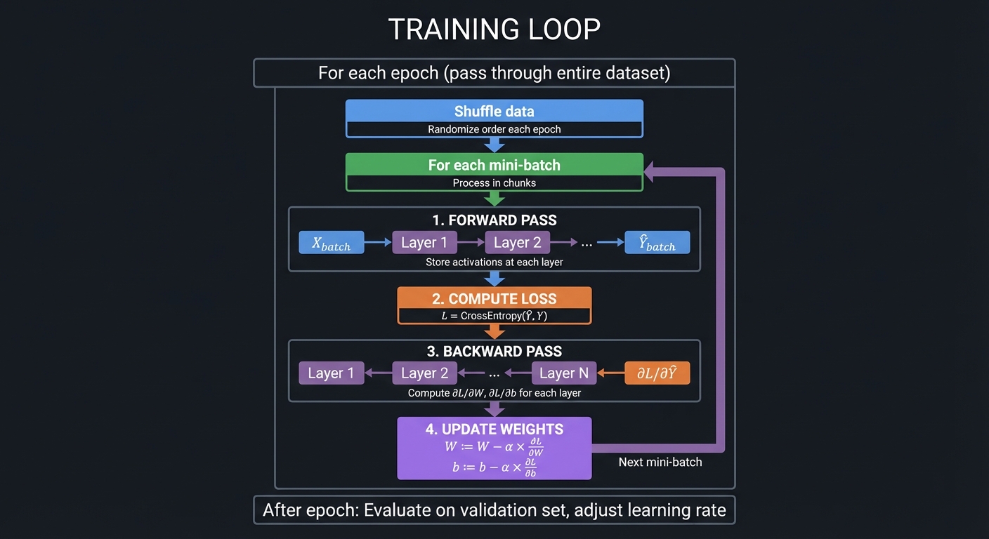
Training Loop Flow
┌─────────────────────────────────────────────────────────────────────────┐
│                         TRAINING LOOP                                   │
├─────────────────────────────────────────────────────────────────────────┤
│                                                                         │
│  For each epoch (pass through entire dataset):                         │
│  ─────────────────────────────────────────────                         │
│                                                                         │
│  ┌─────────────┐                                                        │
│  │ Shuffle data│ Randomize order each epoch                            │
│  └──────┬──────┘                                                        │
│         │                                                               │
│         ▼                                                               │
│  ┌─────────────┐                                                        │
│  │ For each    │ Process in mini-batches                               │
│  │ mini-batch  │                                                        │
│  └──────┬──────┘                                                        │
│         │                                                               │
│         ▼                                                               │
│  ┌─────────────────────────────────────────────────────────────┐       │
│  │ 1. FORWARD PASS                                              │       │
│  │    X_batch ──→ Layer 1 ──→ Layer 2 ──→ ... ──→ Ŷ_batch      │       │
│  │    Store activations at each layer                          │       │
│  └──────┬──────────────────────────────────────────────────────┘       │
│         │                                                               │
│         ▼                                                               │
│  ┌─────────────────────────────────────────────────────────────┐       │
│  │ 2. COMPUTE LOSS                                              │       │
│  │    L = CrossEntropy(Ŷ_batch, Y_batch)                        │       │
│  └──────┬──────────────────────────────────────────────────────┘       │
│         │                                                               │
│         ▼                                                               │
│  ┌─────────────────────────────────────────────────────────────┐       │
│  │ 3. BACKWARD PASS                                             │       │
│  │    ∂L/∂Ŷ ←── Layer N ←── ... ←── Layer 1                    │       │
│  │    Compute ∂L/∂W, ∂L/∂b for each layer                       │       │
│  └──────┬──────────────────────────────────────────────────────┘       │
│         │                                                               │
│         ▼                                                               │
│  ┌─────────────────────────────────────────────────────────────┐       │
│  │ 4. UPDATE WEIGHTS                                            │       │
│  │    W := W - α × ∂L/∂W                                        │       │
│  │    b := b - α × ∂L/∂b                                        │       │
│  └──────┬──────────────────────────────────────────────────────┘       │
│         │                                                               │
│         └──→ Next mini-batch                                            │
│                                                                         │
│  After epoch: Evaluate on validation set, adjust learning rate         │
│                                                                         │
└─────────────────────────────────────────────────────────────────────────┘
Phased Implementation Guide
Phase 1: Data Loading and Preprocessing (Days 1-2)
Goal: Load MNIST and prepare for training
Tasks:
- Download/load MNIST dataset (use keras.datasets or fetch manually)
- Normalize pixel values to [0, 1] or [-1, 1]
- Flatten images from 28×28 to 784-element vectors
- One-hot encode labels
- Create batch iterator
Implementation:
def load_mnist():
    # Using keras for convenience
    from tensorflow.keras.datasets import mnist
    (x_train, y_train), (x_test, y_test) = mnist.load_data()

    # Normalize to [0, 1]
    x_train = x_train.reshape(-1, 784).T / 255.0  # (784, N)
    x_test = x_test.reshape(-1, 784).T / 255.0

    # One-hot encode
    y_train_onehot = np.zeros((10, len(y_train)))
    y_train_onehot[y_train, np.arange(len(y_train))] = 1

    return x_train, y_train_onehot, x_test, y_test
Verification:
# Check shapes
assert x_train.shape == (784, 60000)
assert y_train_onehot.shape == (10, 60000)

# Check normalization
assert x_train.min() >= 0 and x_train.max() <= 1

# Check one-hot
assert y_train_onehot.sum(axis=0).all() == 1  # each column sums to 1
Phase 2: Activation Functions (Days 3-4)
Goal: Implement all activation functions and derivatives
Tasks:
- Implement ReLU and its derivative
- Implement sigmoid and its derivative
- Implement softmax
- Implement cross-entropy loss
Implementation:
def relu(z):
    return np.maximum(0, z)

def relu_derivative(z):
    return (z > 0).astype(float)

def sigmoid(z):
    return 1 / (1 + np.exp(-np.clip(z, -500, 500)))

def sigmoid_derivative(z):
    s = sigmoid(z)
    return s * (1 - s)

def softmax(z):
    # Subtract max for numerical stability
    exp_z = np.exp(z - z.max(axis=0, keepdims=True))
    return exp_z / exp_z.sum(axis=0, keepdims=True)

def cross_entropy_loss(y_pred, y_true):
    # Avoid log(0)
    epsilon = 1e-15
    y_pred = np.clip(y_pred, epsilon, 1 - epsilon)
    return -np.sum(y_true * np.log(y_pred)) / y_true.shape[1]
Verification:
# ReLU
assert relu(np.array([-1, 0, 1])) == [0, 0, 1]
assert relu_derivative(np.array([-1, 0, 1])) == [0, 0, 1]

# Softmax sums to 1
z = np.random.randn(10, 5)
assert np.allclose(softmax(z).sum(axis=0), 1)

# Sigmoid is in (0, 1)
assert (sigmoid(z) > 0).all() and (sigmoid(z) < 1).all()
Phase 3: Forward Propagation (Days 5-7)
Goal: Implement forward pass through network
Tasks:
- Implement Layer forward pass
- Implement Network forward pass
- Verify with known inputs
Implementation:
class Layer:
    def forward(self, X):
        self.input = X
        self.z = self.W @ X + self.b
        if self.activation == 'relu':
            self.a = relu(self.z)
        elif self.activation == 'sigmoid':
            self.a = sigmoid(self.z)
        elif self.activation == 'softmax':
            self.a = softmax(self.z)
        return self.a

class NeuralNetwork:
    def forward(self, X):
        current = X
        for layer in self.layers:
            current = layer.forward(current)
        return current
Verification:
# Initialize network
net = NeuralNetwork([784, 128, 10], ['relu', 'softmax'])

# Forward pass should produce valid probabilities
output = net.forward(x_train[:, :32])
assert output.shape == (10, 32)
assert np.allclose(output.sum(axis=0), 1)
Phase 4: Backpropagation (Days 8-11)
Goal: Implement backward pass for gradient computation
Tasks:
- Implement output layer gradient (softmax + cross-entropy)
- Implement hidden layer backward pass
- Chain gradients through network
- Verify with numerical gradient checking
Implementation:
class Layer:
    def backward(self, dL_da):
        # Gradient through activation
        if self.activation == 'relu':
            dL_dz = dL_da * relu_derivative(self.z)
        elif self.activation == 'sigmoid':
            dL_dz = dL_da * sigmoid_derivative(self.z)
        elif self.activation == 'softmax':
            # For softmax + cross-entropy, gradient simplifies to (ŷ - y)
            dL_dz = dL_da  # Pass dL_da directly (see note below)

        # Gradients for parameters
        batch_size = self.input.shape[1]
        self.dW = dL_dz @ self.input.T / batch_size
        self.db = dL_dz.mean(axis=1, keepdims=True)

        # Gradient to pass to previous layer
        dL_dx = self.W.T @ dL_dz
        return dL_dx

class NeuralNetwork:
    def backward(self, Y):
        # Output layer: softmax + cross-entropy derivative is (ŷ - y)
        dL_da = self.layers[-1].a - Y

        # Backpropagate through layers
        for layer in reversed(self.layers):
            dL_da = layer.backward(dL_da)
Numerical Gradient Check:
def numerical_gradient(f, W, epsilon=1e-5):
    """Compute gradient numerically for verification."""
    grad = np.zeros_like(W)
    for i in range(W.shape[0]):
        for j in range(W.shape[1]):
            W[i, j] += epsilon
            f_plus = f()
            W[i, j] -= 2 * epsilon
            f_minus = f()
            W[i, j] += epsilon  # restore
            grad[i, j] = (f_plus - f_minus) / (2 * epsilon)
    return grad

# Compare analytical vs numerical gradient
# They should match within 1e-5 relative error
Phase 5: Training (Days 12-14)
Goal: Train the network to classify digits
Tasks:
- Implement SGD update step
- Implement training loop
- Track and plot loss over epochs
- Implement evaluation on test set
Implementation:
def train_epoch(net, X, Y, batch_size, learning_rate):
    """Train for one epoch."""
    n_samples = X.shape[1]
    indices = np.random.permutation(n_samples)
    total_loss = 0

    for start in range(0, n_samples, batch_size):
        end = min(start + batch_size, n_samples)
        batch_idx = indices[start:end]

        X_batch = X[:, batch_idx]
        Y_batch = Y[:, batch_idx]

        # Forward
        output = net.forward(X_batch)

        # Loss
        loss = cross_entropy_loss(output, Y_batch)
        total_loss += loss * (end - start)

        # Backward
        net.backward(Y_batch)

        # Update
        for layer in net.layers:
            layer.W -= learning_rate * layer.dW
            layer.b -= learning_rate * layer.db

    return total_loss / n_samples

def evaluate(net, X, y):
    """Compute accuracy."""
    predictions = net.forward(X).argmax(axis=0)
    return (predictions == y).mean()
Training Loop:
net = NeuralNetwork([784, 128, 64, 10], ['relu', 'relu', 'softmax'])

for epoch in range(20):
    loss = train_epoch(net, x_train, y_train_onehot, batch_size=32, learning_rate=0.1)
    acc = evaluate(net, x_test, y_test)
    print(f"Epoch {epoch}: Loss = {loss:.4f}, Test Accuracy = {acc:.4f}")
Phase 6: Visualization and Analysis (Days 15-17)
Goal: Understand what the network learned
Tasks:
- Plot training loss curve
- Visualize first layer weights as images
- Show example predictions with confidence
- Analyze misclassified examples
Visualizations:
# Weight visualization
def visualize_weights(W):
    """Plot first layer weights as 28×28 images."""
    n_neurons = min(W.shape[0], 25)
    fig, axes = plt.subplots(5, 5, figsize=(10, 10))
    for i, ax in enumerate(axes.flat):
        if i < n_neurons:
            img = W[i].reshape(28, 28)
            ax.imshow(img, cmap='RdBu')
        ax.axis('off')
    plt.show()

# Prediction examples
def show_predictions(net, X, y, n=10):
    """Show predictions with confidence."""
    probs = net.forward(X[:, :n])
    preds = probs.argmax(axis=0)
    for i in range(n):
        print(f"True: {y[i]}, Pred: {preds[i]}, Confidence: {probs[preds[i], i]:.2%}")
Phase 7: Improvements and Extensions (Days 18-21)
Goal: Improve accuracy and add features
Tasks:
- Add momentum to SGD
- Implement learning rate decay
- Add dropout regularization
- Experiment with architecture
Momentum SGD:
class MomentumSGD:
    def __init__(self, learning_rate, momentum=0.9):
        self.lr = learning_rate
        self.momentum = momentum
        self.velocities = {}

    def update(self, layer, layer_id):
        if layer_id not in self.velocities:
            self.velocities[layer_id] = {
                'W': np.zeros_like(layer.W),
                'b': np.zeros_like(layer.b)
            }

        v = self.velocities[layer_id]
        v['W'] = self.momentum * v['W'] - self.lr * layer.dW
        v['b'] = self.momentum * v['b'] - self.lr * layer.db

        layer.W += v['W']
        layer.b += v['b']
Testing Strategy
Unit Tests
- Activation functions:
- ReLU(negative) = 0
- Softmax sums to 1
- Sigmoid ∈ (0, 1)
- Forward pass:
- Output shape matches expected
- Probabilities sum to 1
- Backward pass:
- Gradients match numerical approximation
- Shapes are consistent
- Update step:
- Loss decreases on same batch
- Weights actually change
Integration Tests
- Overfit small batch: Should achieve 100% accuracy
- Training curve: Loss should decrease
- Gradient check: Analytical ≈ numerical
Performance Tests
- Target accuracy: >95% on test set
- Training time: Reasonable (minutes, not hours)
- Memory usage: Fits in RAM
Common Pitfalls and Debugging
Shape Mismatches
Symptom: “Shapes not aligned” errors
Cause: Matrix dimensions don’t match for multiplication
Fix: Draw out dimensions at each step:
X:      (784, 32)
W¹:     (128, 784)
W¹ @ X: (128, 32) ✓

dL_dz:  (128, 32)
X.T:    (32, 784)
dW:     (128, 32) @ (32, 784) = (128, 784) ✓
Vanishing/Exploding Gradients
Symptom: Weights become NaN or don’t change
Cause: Improper initialization or unstable activations
Fix:
- Use Xavier/He initialization
- Use ReLU instead of sigmoid for hidden layers
- Gradient clipping:
grad = np.clip(grad, -1, 1)
Numerical Instability
Symptom: NaN in loss or activations
Cause: Overflow in exp(), log(0)
Fix:
# Softmax: subtract max
exp_z = np.exp(z - z.max(axis=0, keepdims=True))

# Cross-entropy: clip predictions
y_pred = np.clip(y_pred, 1e-15, 1 - 1e-15)
Learning Rate Issues
Symptom: Loss oscillates or doesn’t decrease
Cause: Learning rate too high or too low
Fix: Start with 0.01-0.1, use learning rate finder, or adaptive optimizers
Batch Size Effects
Symptom: Different results with different batch sizes
Cause: Gradients not averaged correctly
Fix: Divide gradients by batch size:
self.dW = dL_dz @ self.input.T / batch_size
Extensions and Challenges
Beginner Extensions
- Add L2 regularization (weight decay)
- Implement early stopping
- Save/load model weights
Intermediate Extensions
- Implement Adam optimizer
- Add batch normalization
- Implement dropout
- Try different architectures
Advanced Extensions
- Implement convolutional layers
- Add residual connections
- Implement in pure C
- GPU acceleration with CUDA
Real-World Connections
Deep Learning Frameworks
Every framework (PyTorch, TensorFlow, JAX) does exactly this:
- Forward pass: compute outputs
- Backward pass: compute gradients (autograd)
- Update: optimizer step
Understanding the math lets you debug and optimize effectively.
Computer Vision
This MNIST classifier is a simplified version of:
- Handwriting recognition (postal services)
- OCR (document scanning)
- Medical image analysis
- Self-driving cars
Natural Language Processing
Same principles apply:
- Word embeddings are learned weight matrices
- Transformers use attention (matrix operations)
- Language models predict next tokens (classification)
Optimization Theory
Gradient descent connects to:
- Convex optimization
- Stochastic approximation
- Online learning
Self-Assessment Checklist
Conceptual Understanding
- I can explain why neural networks need nonlinearity
- I understand what each matrix multiplication represents
- I can derive the backpropagation equations
- I know why the transpose appears in gradients
- I understand the role of learning rate and batch size
Practical Skills
- I implemented forward propagation with matrix operations
- I implemented backpropagation from scratch
- My network achieves >95% accuracy on MNIST
- I can visualize and interpret learned weights
- I can debug shape mismatch errors
Teaching Test
Can you explain to someone else:
- How does a single neuron compute its output?
- What does each layer learn?
- Why do we use mini-batches?
- How does backpropagation work?
Resources
Primary
- “Math for Programmers” by Paul Orland - Chapter on ML
- 3Blue1Brown: Neural Networks - Visual intuition
- “Grokking Algorithms” - ML appendix
Reference
- “Deep Learning” by Goodfellow, Bengio, Courville - The definitive textbook
- “Hands-On Machine Learning” by Aurélien Géron - Practical guide
- CS231n course notes (Stanford) - Detailed derivations
Code References
- NumPy documentation - Matrix operations
- micrograd by Andrej Karpathy - Minimal autograd implementation
- PyTorch source code - Production implementation
When you complete this project, you’ll understand that deep learning is not magic—it’s linear algebra composed with nonlinearities, optimized via calculus. Every AI breakthrough is built on these foundations you now understand.