P02: Image Compression Using SVD
Build a tool that compresses images by decomposing them with Singular Value Decomposition, letting you visually see how much information each “rank” captures.
Overview
| Attribute | Value |
|---|---|
| Difficulty | Intermediate |
| Time Estimate | 1-2 weeks |
| Language | Python (recommended) or C |
| Prerequisites | Basic matrix operations, understanding of P01 |
| Primary Book | “Math for Programmers” by Paul Orland |
Learning Objectives
By completing this project, you will:
- See matrices as data - Understand that any grid of numbers (images, spreadsheets) is a matrix
- Master matrix decomposition - Break matrices into simpler, meaningful components
- Understand eigenvalues intuitively - The “importance weights” of a matrix’s structure
- Grasp low-rank approximation - How a few numbers can capture most information
- Connect SVD to applications - Compression, recommendation systems, dimensionality reduction
- Build numerical intuition - Understand floating-point precision and numerical stability
Theoretical Foundation
Part 1: Images as Matrices
The Digital Image
A grayscale image is nothing more than a matrix of numbers:
┌────────────────────────────────────────────────────────────────┐
│                    GRAYSCALE IMAGE AS MATRIX                   │
├────────────────────────────────────────────────────────────────┤
│                                                                │
│    Image (visual)              Matrix (numerical)              │
│                                                                │
│    ░░░░██████░░░░             [0   0   0   0   128 128 128 ... │
│    ░░████████░░░░              0   0   128 128 255 255 255 ... │
│    ░░████████░░░░              0   0   128 128 255 255 255 ... │
│    ░░██░░░░██░░░░              0   0   128 0   0   0   128 ... │
│    ░░░░░░░░░░░░░░              0   0   0   0   0   0   0   ... │
│                                        ...                     │
│                                                                │
│    Each pixel = one matrix entry                               │
│    Value 0-255 represents darkness to brightness               │
│                                                                │
└────────────────────────────────────────────────────────────────┘
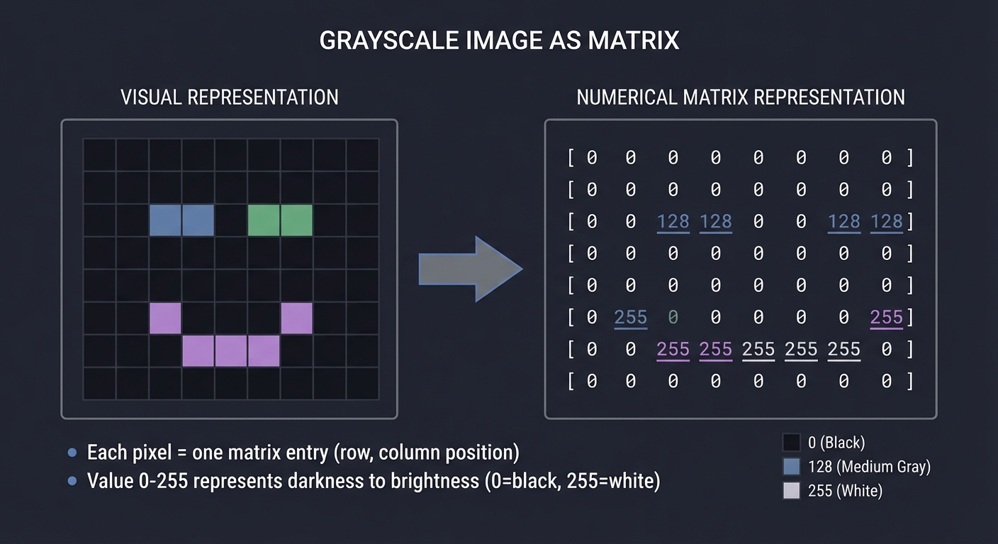
For an m×n image, we have an m×n matrix A where:
- A[i][j] = brightness of pixel at row i, column j
- Typically 0 = black, 255 = white (for 8-bit images)
For color images, we have three matrices: one each for Red, Green, Blue channels.
Matrix Properties
A 512×512 grayscale image:
- 512 × 512 = 262,144 pixels
- Each pixel = 1 byte (8 bits, values 0-255)
- Total: 262,144 bytes ≈ 256 KB

Can we store this with fewer numbers?
Part 2: The Rank of a Matrix
What is Rank?
The rank of a matrix is the number of “truly independent” pieces of information it contains.
Full rank matrix (rank 3):      Low rank matrix (rank 1):

[1  0  0]                       [1  2  3]
[0  1  0]   rank = 3            [2  4  6]   rank = 1
[0  0  1]                       [3  6  9]

Every row/column adds new       All rows are multiples of [1,2,3]
information                     Only ONE piece of information!
Key insight: A rank-1 matrix can be written as the outer product of two vectors:
[1  2  3]     [1]
[2  4  6]  =  [2] × [1  2  3]  =  u × vᵀ
[3  6  9]     [3]

Instead of storing 9 numbers, store 6 numbers (two vectors)!
Rank and Information
- A rank-k matrix can be written as the sum of k rank-1 matrices
- Real images rarely have exact low rank, but are “approximately” low rank
- The important patterns are captured by the first few rank-1 pieces
- The remaining pieces are often noise or fine detail
Full Image ≈ Major patterns + Minor patterns + Finer details + Noise
             (rank 1)         (rank 2-10)     (rank 11-50)    (rest)
Part 3: Eigenvalues and Eigenvectors
The Core Concept
An eigenvector of matrix A is a special direction that only gets stretched (not rotated) by A:
A × v = λ × v

Where:
- v is the eigenvector (a direction in space)
- λ (lambda) is the eigenvalue (the stretch factor)
Visually:
                    A transforms...

Regular vector:     →  gets rotated AND stretched
Eigenvector:        →  gets ONLY stretched (by factor λ)

If λ = 2:  eigenvector doubles in length
If λ = 0.5: eigenvector halves
If λ = -1: eigenvector flips direction
If λ = 0:  eigenvector collapses to zero
Why Eigenvectors Matter
Eigenvectors reveal the natural axes of a transformation:
Consider stretching an image 2× horizontally, 0.5× vertically:

          [2   0]
Stretch = [0  0.5]

Eigenvectors: [1, 0] with λ=2    (horizontal direction)
              [0, 1] with λ=0.5  (vertical direction)

These are the "natural" directions of the transformation!
For symmetric matrices (like AᵀA), eigenvectors are orthogonal—they form a new coordinate system aligned with the matrix’s “preferred” directions.
Eigenvalue Magnitude
The magnitude of an eigenvalue indicates importance:
-
Large λ : This direction is strongly affected by the transformation -
Small λ : This direction is weakly affected - λ = 0: This direction is completely nullified (in the null space)
Part 4: Singular Value Decomposition (SVD)
The Grand Decomposition
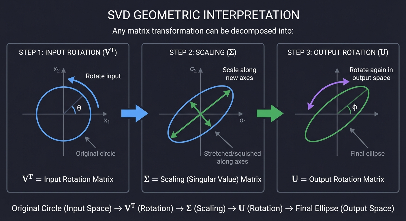
SVD says: Every matrix can be written as a sequence of three simple operations.
A = U × Σ × Vᵀ

Where:
- U: m×m orthogonal matrix (rotation in output space)
- Σ: m×n diagonal matrix (scaling)
- Vᵀ: n×n orthogonal matrix (rotation in input space)

For an m×n matrix A.
Geometrically:
┌─────────────────────────────────────────────────────────────────────────┐
│                      SVD GEOMETRIC INTERPRETATION                       │
├─────────────────────────────────────────────────────────────────────────┤
│                                                                         │
│    Any matrix transformation can be decomposed into:                    │
│                                                                         │
│    Vᵀ           Σ              U                                        │
│    ───────  →  ─────────  →   ───────                                   │
│    Rotate      Scale along    Rotate again                              │
│    input       new axes       in output space                           │
│                                                                         │
│    ○             ⬭              ⬭                                       │
│   ╱│╲    →     ╱   ╲     →    ╱    ╲                                    │
│    │             │               ╲                                      │
│    ↑             ↑                ↖                                     │
│                                                                         │
│    Original   Stretched/       Final                                    │
│    circle     squished         ellipse                                  │
│               along axes                                                │
│                                                                         │
└─────────────────────────────────────────────────────────────────────────┘
The Components
Σ (Sigma) - The Singular Values:
        [σ₁  0   0  ...]
    Σ = [0   σ₂  0  ...]
        [0   0   σ₃ ...]
        [... ... ... ]

- σ₁ ≥ σ₂ ≥ σ₃ ≥ ... ≥ 0 (ordered by magnitude)
- These are the square roots of eigenvalues of AᵀA
- They measure the "importance" of each component
U - Left Singular Vectors:
- Columns of U are orthonormal vectors in the output space
- They form the new coordinate axes after transformation
- u₁ is the most “stretched” direction
V - Right Singular Vectors:
- Columns of V are orthonormal vectors in the input space
- They are the input directions that become the U directions
- Av₁ points in the u₁ direction (scaled by σ₁)
SVD as Sum of Rank-1 Matrices
The magical property:
A = σ₁(u₁ × v₁ᵀ) + σ₂(u₂ × v₂ᵀ) + σ₃(u₃ × v₃ᵀ) + ...

Each term (uᵢ × vᵢᵀ) is a rank-1 matrix!
Each σᵢ is the "weight" or importance of that term.
For images:
Image = σ₁(pattern₁) + σ₂(pattern₂) + σ₃(pattern₃) + ...

Where σ₁ > σ₂ > σ₃ > ...

The first few patterns capture most of the image!
Part 5: Low-Rank Approximation
The Eckart-Young-Mirsky Theorem
This is the key result that makes SVD useful for compression:
The best rank-k approximation to A is obtained by keeping only the top k singular values.
A_k = σ₁(u₁ × v₁ᵀ) + σ₂(u₂ × v₂ᵀ) + ... + σₖ(uₖ × vₖᵀ)

This is the closest rank-k matrix to A (in terms of Frobenius norm).
No other rank-k matrix is closer!
Compression Achieved
For an m×n image with rank-k approximation:
Original storage: m × n values

SVD storage (rank k):
- k columns of U: m × k values
- k singular values: k values
- k columns of V: n × k values
Total: k × (m + n + 1) values

Compression ratio: (m × n) / (k × (m + n + 1))
Example with 512×512 image:
Original: 262,144 values

Rank 10:  10 × (512 + 512 + 1) = 10,250 values
Compression: 25.6× smaller!

Rank 50:  50 × 1,025 = 51,250 values
Compression: 5.1× smaller!
Choosing k
How many singular values to keep?
┌────────────────────────────────────────────────────────────────┐
│                    SINGULAR VALUE DECAY                        │
├────────────────────────────────────────────────────────────────┤
│                                                                │
│  σ                                                             │
│  │                                                             │
│  │█                                                            │
│  │█                                                            │
│  │██                                                           │
│  │███                                                          │
│  │████                                                         │
│  │██████                                                       │
│  │█████████                                                    │
│  │████████████████████████████████████──────────────           │
│  └──────────────────────────────────────────────────── k       │
│     ↑           ↑                    ↑                         │
│     keep these  cutoff               discard these             │
│     (signal)    here                 (noise/detail)            │
│                                                                │
└────────────────────────────────────────────────────────────────┘
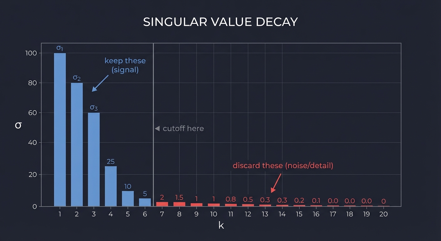
Common criteria:
- Keep k values that capture X% of total “energy”:
(σ₁² + σ₂² + ... + σₖ²) / (σ₁² + σ₂² + ... + σₙ²) ≥ X% - Keep values above a threshold
- Fixed k based on desired file size
Part 6: Computing SVD
Method 1: Via Eigendecomposition
For matrix A, compute:
- AᵀA (symmetric positive semi-definite)
- Find eigenvalues λᵢ and eigenvectors vᵢ of AᵀA
- Singular values: σᵢ = √λᵢ
- V = [v₁, v₂, …, vₙ]
- U columns: uᵢ = Avᵢ / σᵢ
This works but has numerical issues for large matrices.
Method 2: Power Iteration (for largest singular value)
def largest_singular_value(A, iterations=100):
    v = random_unit_vector(n)
    for _ in range(iterations):
        u = A @ v           # Apply A
        u = u / norm(u)     # Normalize
        v = A.T @ u         # Apply Aᵀ
        v = v / norm(v)     # Normalize
    sigma = norm(A @ v)
    return sigma, u, v
This finds σ₁, u₁, v₁. For subsequent singular values, deflate: A₂ = A - σ₁u₁v₁ᵀ
Method 3: Use a Library
In practice, use optimized implementations:
import numpy as np
U, S, Vt = np.linalg.svd(A, full_matrices=False)
Part 7: Image-Specific Considerations
Color Images
For RGB images, apply SVD to each channel separately:
Original: R, G, B channels (each m×n)

For each channel:
  U_c, Σ_c, V_c = SVD(channel)
  compressed_c = U_c[:, :k] @ Σ_c[:k, :k] @ V_c[:k, :]

Reconstruct: Combine compressed R, G, B
Or convert to YCbCr and compress more aggressively on chrominance channels (human eyes are less sensitive to color detail).
Block-Based Compression
Like JPEG, process image in blocks:
For each 8×8 or 16×16 block:
  Apply SVD
  Keep top k singular values
  Store U, Σ, V for block
This allows local adaptation and parallelization.
Comparison with Other Methods
| Method | Approach | SVD Similarity |
|---|---|---|
| JPEG | DCT + quantization | Both find basis; DCT uses fixed basis |
| PCA | Find principal components | PCA of rows = SVD (related) |
| Wavelets | Multi-resolution decomposition | Different basis functions |
Project Specification
What You’re Building
A command-line tool that:
- Loads a grayscale or color image
- Computes SVD of the image matrix
- Reconstructs the image using top k singular values
- Displays/saves the compressed image
- Reports compression ratio and quality metrics
Minimum Requirements
- Load image as matrix (grayscale first)
- Compute SVD (use library or implement)
- Reconstruct image with top k singular values
- Display original vs compressed side-by-side
- Calculate and display compression ratio
- Allow user to specify k
- Show singular value decay plot
Stretch Goals
- Support color images (per-channel SVD)
- Implement SVD from scratch (power iteration)
- Interactive slider to adjust k in real-time
- Calculate PSNR/SSIM quality metrics
- Compare with JPEG at similar file sizes
- Save compressed representation to file
Solution Architecture
Data Structures
class SVDCompressor:
    """Handles SVD-based image compression."""

    def __init__(self, image: np.ndarray):
        self.original = image
        self.U = None
        self.S = None  # Singular values
        self.Vt = None

    def compress(self, k: int) -> np.ndarray:
        """Return rank-k approximation."""
        pass

    def compression_ratio(self, k: int) -> float:
        """Calculate storage ratio."""
        pass

    def energy_captured(self, k: int) -> float:
        """Percentage of total variance captured."""
        pass
Module Structure
┌─────────────────────────────────────────────────────────────────┐
│                           main.py                               │
│  - CLI argument parsing                                         │
│  - Load image                                                   │
│  - Display results                                              │
└─────────────────────────────────────────────────────────────────┘
                               │
        ┌──────────────────────┼──────────────────────┐
        ▼                      ▼                      ▼
┌──────────────┐      ┌──────────────┐      ┌──────────────┐
│   image.py   │      │    svd.py    │      │  metrics.py  │
│              │      │              │      │              │
│ load_image   │      │ compute_svd  │      │ psnr         │
│ save_image   │      │ reconstruct  │      │ ssim         │
│ display      │      │ truncate     │      │ compression_ratio │
│ to_grayscale │      │              │      │ energy_ratio │
└──────────────┘      └──────────────┘      └──────────────┘
                               │
                               ▼
                      ┌──────────────┐
                      │  visualize.py│
                      │              │
                      │ plot_singular_values │
                      │ side_by_side │
                      │ difference_image │
                      └──────────────┘
Processing Pipeline
┌─────────────────────────────────────────────────────────────────────────┐
│                        SVD COMPRESSION PIPELINE                         │
├─────────────────────────────────────────────────────────────────────────┤
│                                                                         │
│  ┌─────────────┐                                                        │
│  │ Input Image │  512×512 grayscale                                     │
│  │ (m × n)     │  262,144 values                                        │
│  └──────┬──────┘                                                        │
│         │                                                               │
│         ▼  Compute SVD                                                  │
│  ┌─────────────────────────────────────────────────┐                   │
│  │ A = U × Σ × Vᵀ                                   │                   │
│  │                                                  │                   │
│  │ U: 512×512    Σ: 512×512 diagonal    Vᵀ: 512×512│                   │
│  └──────┬──────────────┬───────────────────┬───────┘                   │
│         │              │                   │                            │
│         ▼              ▼                   ▼                            │
│  ┌──────────┐   ┌────────────┐      ┌──────────┐                       │
│  │ Keep top │   │ Keep top   │      │ Keep top │                       │
│  │ k columns│   │ k values   │      │ k rows   │                       │
│  │ of U     │   │ of Σ       │      │ of Vᵀ    │                       │
│  └──────────┘   └────────────┘      └──────────┘                       │
│         │              │                   │                            │
│         └──────────────┼───────────────────┘                            │
│                        ▼                                                │
│              ┌─────────────────┐                                        │
│              │ Reconstruct     │                                        │
│              │ A_k = U_k Σ_k V_k^T │                                   │
│              └────────┬────────┘                                        │
│                       │                                                 │
│                       ▼                                                 │
│              ┌─────────────────┐                                        │
│              │ Compressed Image│  k = 50: 51,250 values                 │
│              │ (rank k approx) │  5× compression                        │
│              └─────────────────┘                                        │
│                                                                         │
└─────────────────────────────────────────────────────────────────────────┘

Phased Implementation Guide
Phase 1: Image Loading and Display (Days 1-2)
Goal: Load and display images as matrices
Tasks:
- Set up Python environment with numpy, PIL/OpenCV, matplotlib
- Load grayscale image as numpy array
- Display image using matplotlib
- Print matrix dimensions and value range
- Visualize raw matrix values (maybe a small crop)
Verification:
# Image should load as 2D array
assert len(image.shape) == 2  # grayscale
assert image.min() >= 0 and image.max() <= 255

# Display should show correct image
plt.imshow(image, cmap='gray')
Phase 2: SVD Computation (Days 3-4)
Goal: Compute and understand SVD components
Tasks:
- Compute SVD using
np.linalg.svd() - Verify: reconstruct original from U, S, Vt
- Plot singular values (should decay)
- Calculate energy captured by top k values
Verification:
U, S, Vt = np.linalg.svd(image, full_matrices=False)

# Reconstruct should equal original
reconstructed = U @ np.diag(S) @ Vt
assert np.allclose(image, reconstructed)

# Singular values should be non-negative and ordered
assert all(s >= 0 for s in S)
assert all(S[i] >= S[i+1] for i in range(len(S)-1))
Phase 3: Low-Rank Approximation (Days 5-6)
Goal: Reconstruct images with reduced rank
Tasks:
- Implement truncation to rank k
- Reconstruct and display for various k values
- Create side-by-side comparisons
- Calculate compression ratios
Implementation:
def compress(U, S, Vt, k):
    """Reconstruct using only top k singular values."""
    U_k = U[:, :k]
    S_k = S[:k]
    Vt_k = Vt[:k, :]
    return U_k @ np.diag(S_k) @ Vt_k
Verification:
- k=1: Very blurry, single dominant pattern
- k=10: Major features visible
- k=50: Good quality for most images
- k=full: Equals original
Phase 4: Visualization (Days 7-8)
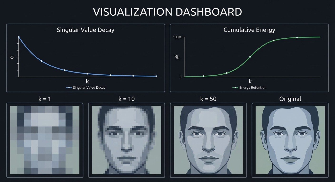
Goal: Create informative visualizations
Tasks:
- Plot singular value decay (log scale useful)
- Show cumulative energy curve
- Display rank-1, rank-10, rank-50, original side by side
- Create difference image (original - compressed)
- Implement interactive slider for k
Visualizations:
┌────────────────────────────────────────────────────────────────┐
│                   VISUALIZATION DASHBOARD                      │
├────────────────────────────────────────────────────────────────┤
│                                                                │
│  ┌─────────────────────────┐  ┌─────────────────────────┐     │
│  │ Singular Value Decay    │  │ Cumulative Energy       │     │
│  │                         │  │                         │     │
│  │  σ                      │  │  %                 100% │     │
│  │  │\                     │  │  │            ____──    │     │
│  │  │ \                    │  │  │        ___/          │     │
│  │  │  \_____              │  │  │    ___/              │     │
│  │  └──────────── k        │  │  └───/──────────── k    │     │
│  │                         │  │                         │     │
│  └─────────────────────────┘  └─────────────────────────┘     │
│                                                                │
│  ┌───────────┐ ┌───────────┐ ┌───────────┐ ┌───────────┐      │
│  │  k = 1    │ │  k = 10   │ │  k = 50   │ │ Original  │      │
│  │           │ │           │ │           │ │           │      │
│  │   ▒▒▒▒    │ │   ▓▓▒▒    │ │   ████    │ │   ████    │      │
│  │   ▒▒▒▒    │ │   ▓▓▒▒    │ │   ████    │ │   ████    │      │
│  │           │ │           │ │           │ │           │      │
│  └───────────┘ └───────────┘ └───────────┘ └───────────┘      │
│                                                                │
└────────────────────────────────────────────────────────────────┘
Phase 5: Metrics and Analysis (Days 9-10)
Goal: Quantify compression quality
Tasks:
- Implement PSNR (Peak Signal-to-Noise Ratio)
- Implement MSE (Mean Squared Error)
- Calculate compression ratios for various k
- Create quality vs. compression tradeoff plot
- Compare with JPEG at similar sizes
Metrics:
def mse(original, compressed):
    return np.mean((original - compressed) ** 2)

def psnr(original, compressed, max_val=255):
    return 10 * np.log10(max_val**2 / mse(original, compressed))

# PSNR > 30 dB: Good quality
# PSNR > 40 dB: Excellent quality
Phase 6: Color Images (Days 11-12)
Goal: Extend to RGB images
Tasks:
- Load color image and split into R, G, B channels
- Apply SVD to each channel
- Reconstruct each channel
- Combine channels and display
- Compare different k for each channel
Implementation:
def compress_color(image, k):
    channels = [image[:,:,i] for i in range(3)]
    compressed = []
    for channel in channels:
        U, S, Vt = np.linalg.svd(channel, full_matrices=False)
        compressed.append(compress(U, S, Vt, k))
    return np.stack(compressed, axis=2)
Phase 7: Optional - Implement SVD from Scratch (Days 13-14)
Goal: Understand the algorithm deeply
Tasks:
- Implement power iteration for largest singular value
- Implement matrix deflation
- Compute multiple singular values iteratively
- Compare results with numpy
Implementation:
def power_iteration(A, num_iters=100):
    """Find largest singular value and vectors."""
    m, n = A.shape
    v = np.random.randn(n)
    v = v / np.linalg.norm(v)

    for _ in range(num_iters):
        u = A @ v
        u = u / np.linalg.norm(u)
        v = A.T @ u
        v = v / np.linalg.norm(v)

    sigma = np.linalg.norm(A @ v)
    return sigma, u, v

def svd_manual(A, k):
    """Compute top k singular values via power iteration."""
    singular_values = []
    U_cols, V_cols = [], []
    A_remaining = A.copy()

    for _ in range(k):
        sigma, u, v = power_iteration(A_remaining)
        singular_values.append(sigma)
        U_cols.append(u)
        V_cols.append(v)
        A_remaining = A_remaining - sigma * np.outer(u, v)

    return np.array(U_cols).T, np.array(singular_values), np.array(V_cols)
Testing Strategy
Unit Tests
- SVD reconstruction:
- Full reconstruction should equal original (within floating point tolerance)
- Singular value properties:
- All singular values ≥ 0
- Sorted in descending order
- Count ≤ min(m, n)
- Orthogonality:
- U columns should be orthonormal: UᵀU = I
- V columns should be orthonormal: VᵀV = I
- Rank-k approximation:
- rank(A_k) ≤ k
- A_k converges to A as k increases
Visual Tests
- Quality progression: k=1 → k=full should show smooth improvement
- No artifacts: Compressed image shouldn’t have obvious visual errors
- Difference image: Should show high-frequency detail removed
Numerical Tests
- Compression ratio: Should match theoretical formula
- Energy capture: Sum of top k σ² / total σ² should increase with k
- PSNR: Should increase with k
Common Pitfalls and Debugging
Numerical Precision
Symptom: Small differences between original and full reconstruction
Cause: Floating-point arithmetic has limited precision
Fix: Use np.allclose() with appropriate tolerance, not exact equality
Image Data Type
Symptom: Image looks wrong or values are clipped
Cause: Image loaded as uint8 (0-255) but SVD produces floats
Fix: Convert to float before SVD, clip to [0, 255] after reconstruction
Memory for Large Images
Symptom: Out of memory for large images
Cause: Full SVD computes all singular values
Fix: Use svd(A, full_matrices=False) for economy SVD, or use randomized SVD
Color Channel Issues
Symptom: Color images have wrong colors after reconstruction
Cause: Channels mixed up or not properly recombined
Fix: Carefully track channel order, ensure float→uint8 conversion is correct
Visualization Scale
Symptom: Compressed image looks too dark or too bright
Cause: Value range not normalized for display
Fix: Clip to valid range, or normalize: (image - min) / (max - min)
Extensions and Challenges
Beginner Extensions
- Save/load compressed representation
- Process multiple images in batch
- Add command-line interface with argparse
Intermediate Extensions
- Implement randomized SVD for large images
- Adaptive k selection based on quality threshold
- Block-based SVD (like JPEG blocks)
- Video compression (SVD on frame differences)
Advanced Extensions
- Implement truncated SVD with Lanczos algorithm
- Compare with DCT-based compression
- Explore tensor decomposition for color images
- GPU acceleration with CuPy or PyTorch
Real-World Connections
Data Compression
SVD is the mathematical foundation for:
- Netflix’s video encoding (partial)
- Image thumbnails and progressive loading
- Scientific data compression
Recommendation Systems
Netflix Prize (2006-2009) used matrix factorization:
Ratings Matrix ≈ U × Σ × Vᵀ

U rows: user latent factors (taste preferences)
V rows: item latent factors (movie characteristics)
Σ: importance weights
Your image compression is training you for this!
Dimensionality Reduction
PCA (Principal Component Analysis) is closely related:
Centered data matrix X
PCA directions = right singular vectors of X
PCA scores = left singular vectors × singular values
Natural Language Processing
Latent Semantic Analysis (LSA):
Term-Document Matrix → SVD → Topics

U: term-topic relationships
V: document-topic relationships
Σ: topic importance
Noise Reduction
Small singular values often correspond to noise:
Signal ≈ large singular values
Noise ≈ small singular values

Removing small σᵢ denoises the data!
Self-Assessment Checklist
Conceptual Understanding
- I can explain what a matrix rank means geometrically
- I understand why singular values are ordered
- I can explain the Eckart-Young theorem in simple terms
- I know why low-rank approximation works for compression
- I understand the relationship between SVD and eigendecomposition
Practical Skills
- I can compute SVD and reconstruct the original matrix
- I can choose an appropriate k for a given compression target
- I can measure and interpret compression quality metrics
- I can visualize singular value decay and energy capture
- I can apply SVD compression to color images
Teaching Test
Can you explain to someone else:
- Why can a rank-1 matrix be stored with fewer numbers?
- What do the columns of U and V represent?
- Why are the first singular values larger?
- How does SVD relate to JPEG compression?
Resources
Primary
- “Math for Programmers” by Paul Orland - Practical approach
- 3Blue1Brown: Essence of Linear Algebra - Especially the SVD intuition
- Grokking Algorithms - Appendix on linear algebra
Reference
- “Numerical Linear Algebra” by Trefethen & Bau - Rigorous treatment
- “Mining of Massive Datasets” - SVD for recommendation
- “The Elements of Statistical Learning” - SVD/PCA connection
Online
- NumPy SVD documentation - Implementation details
- Interactive SVD visualizations - Various web apps
- JPEG compression tutorials - For comparison
When you complete this project, you’ll understand that matrices contain hidden structure—and that structure can be extracted, prioritized, and reconstructed. This is the foundation for machine learning, signal processing, and data science.