Sprint: Three.js Mastery - From Blank Canvas to Interactive 3D Worlds
Goal: Master 3D web graphics from first principles using Three.js. You will understand the complete rendering pipeline – scene graphs, cameras, materials, lighting, textures, shaders, physics, and post-processing – and build 13 progressively complex projects from a spinning cube to a full interactive 3D portfolio. By the end you will be able to architect, animate, optimize, and ship production-quality 3D experiences in any modern browser.
Introduction
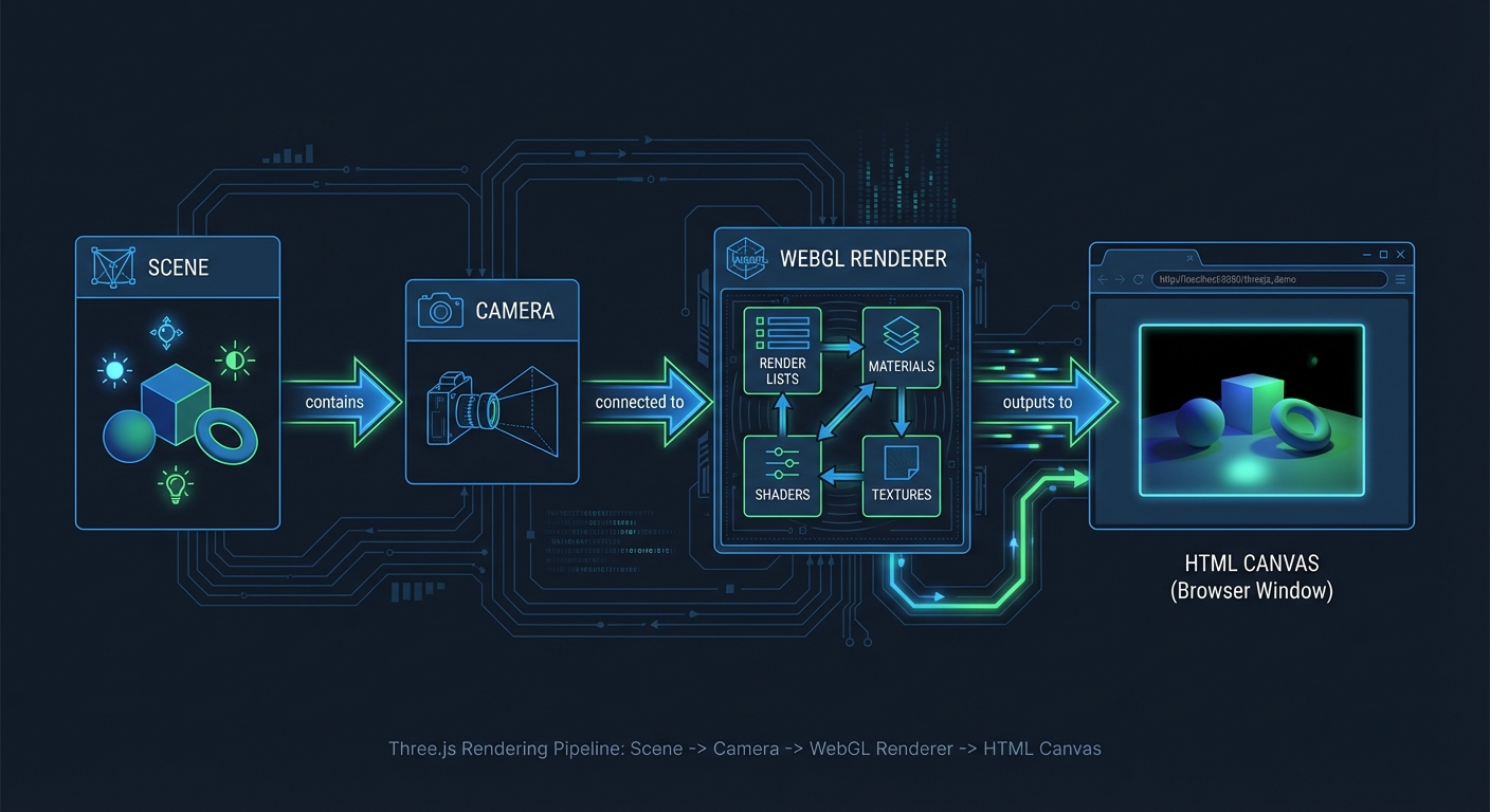
Three.js is a JavaScript library that abstracts the WebGL (and now WebGPU) graphics API into a developer-friendly scene graph. Instead of writing hundreds of lines of raw WebGL boilerplate to place a single triangle on screen, Three.js lets you describe a 3D world in terms of familiar concepts: scenes, cameras, lights, meshes, and materials. Under the hood it translates these high-level descriptions into the low-level GPU commands that WebGL and WebGPU require.
What problem does it solve? WebGL is powerful but brutally verbose. To render a textured cube with raw WebGL you must manually create shader programs, compile GLSL code, allocate GPU buffers, manage transformation matrices, and handle the render loop – easily 200+ lines of boilerplate before anything appears on screen. Three.js collapses that to roughly 15 lines of clear, readable code. It makes 3D accessible to any web developer who knows JavaScript.
Three.js was created by Ricardo Cabello (mrdoob) in 2010 and has grown to over 100,000 GitHub stars with more than 2,000 contributors. It powers 3D experiences at Apple, Nike, Google, NASA, IKEA, Spotify, and thousands of creative studios worldwide. With approximately 3-5 million weekly npm downloads as of early 2026, it is by far the most widely used 3D library for the web – roughly 270 times more downloads than its nearest competitor, Babylon.js. WebGL 2.0 is supported by 97%+ of browsers, and as of late 2025, WebGPU support has landed in all major browsers (Chrome, Firefox, Safari), giving Three.js access to next-generation GPU capabilities.
What will you build across 13 projects?
- A spinning, textured cube with orbit controls (rendering fundamentals)
- A mini solar system with hierarchical orbits (scene graph and transformations)
- A PBR material showcase gallery (materials and lighting)
- A terrain heightmap renderer (geometry, textures, and displacement)
- A haunted house with baked shadows (lighting, shadows, and atmosphere)
- A GLTF model viewer with animation playback (asset loading pipeline)
- A particle galaxy generator (particle systems and GPU animation)
- An ocean water shader (custom GLSL vertex and fragment shaders)
- A physics sandbox with ragdolls (physics engine integration)
- A 3D product configurator (raycasting, interaction, and UI)
- A post-processed cinematic scene (bloom, DOF, color grading)
- A procedural city with 50K buildings (instancing and performance)
- An interactive 3D portfolio website (everything combined)
Scope
In scope:
- Three.js core API (Scene, Camera, Renderer, Mesh, Material, Light, etc.)
- The WebGL rendering pipeline and what happens on the GPU
- GLSL basics: vertex shaders, fragment shaders, uniforms, varyings
- Physics integration (cannon-es and Rapier)
- Post-processing with EffectComposer
- Performance optimization (instancing, LOD, draw call reduction)
- Asset loading (GLTF/GLB, Draco, textures)
- Responsive design and device pixel ratio
Out of scope:
- React Three Fiber (R3F) – a wrapper around Three.js for React apps, not Three.js itself
- 3D modeling in Blender (we use pre-made models; modeling is a separate discipline)
- Production deployment, CI/CD, and hosting infrastructure
- WebXR/VR (a separate specialization)
- Three.js node material system / TSL (Three Shading Language) – bleeding edge, still stabilizing
Why Three.js over alternatives? Babylon.js is a full-featured game engine with built-in physics, audio, and a visual editor. PlayCanvas offers a cloud-based collaborative editor. A-Frame provides HTML-like markup for VR scenes. These are all valid tools. We focus on Three.js because it is the most widely adopted, has the largest ecosystem of tutorials and examples, gives you the most control over the rendering pipeline, and teaches you transferable 3D graphics concepts that apply to any engine or framework. If you understand Three.js deeply, you can pick up any alternative quickly.
The Big Picture: From JavaScript to Pixels
Every Three.js application follows the same pipeline, from your JavaScript code to colored pixels on the HTML canvas:
YOUR JAVASCRIPT CODE
        |
        v
+------------------+     +------------------+     +------------------+
|                  |     |                  |     |                  |
|   Scene Graph    |---->|     Camera       |---->|    Renderer      |
|                  |     |                  |     | (WebGLRenderer)  |
|  - Meshes        |     |  - Projection    |     |                  |
|  - Lights        |     |  - View matrix   |     |  Traverses scene |
|  - Groups        |     |  - Frustum       |     |  Sorts objects   |
|  - Cameras       |     |                  |     |  Issues draw     |
|                  |     |                  |     |  calls to GPU    |
+------------------+     +------------------+     +--------+---------+
                                                           |
                              GPU PIPELINE                 |
                    +--------------------------------------+
                    |
                    v
+------------------+     +------------------+     +------------------+
|                  |     |                  |     |                  |
| Vertex Shader    |---->|  Rasterizer      |---->| Fragment Shader  |
|                  |     |                  |     |                  |
| Runs per-vertex  |     | Converts         |     | Runs per-pixel   |
| Transforms       |     | triangles to     |     | Computes final   |
| positions from   |     | fragments        |     | color using      |
| model space to   |     | (potential       |     | lighting, tex-   |
| clip space       |     |  pixels)         |     | tures, uniforms  |
|                  |     |                  |     |                  |
+------------------+     +------------------+     +--------+---------+
                                                           |
                                                           v
                                              +------------------+
                                              |                  |
                                              |  Framebuffer     |
                                              |                  |
                                              |  Depth testing   |
                                              |  Blending        |
                                              |  Final pixels    |
                                              |                  |
                                              +--------+---------+
                                                       |
                                                       v
                                              +------------------+
                                              |                  |
                                              |  HTML <canvas>   |
                                              |                  |
                                              |  The image you   |
                                              |  see on screen   |
                                              |                  |
                                              +------------------+
This pipeline runs 60 times per second (or more on high-refresh displays). Every frame, Three.js traverses your scene graph, determines what is visible to the camera, and sends drawing instructions to the GPU. The GPU then runs your vertex shader on every vertex, rasterizes the resulting triangles into pixel-sized fragments, runs the fragment shader on each fragment to compute its color, and writes the final image to the canvas.
Understanding this pipeline is the single most important mental model in this entire guide. Every project you build exercises different stages of it. When something goes wrong – a mesh is invisible, a shadow is missing, a material looks flat – you will debug by asking: “which stage of the pipeline is broken?”
Here is a simplified view of the same pipeline as a linear flow, useful for quick mental reference:
JavaScript  -->  Scene + Camera  -->  Renderer traversal  -->  Vertex Shader
     |                                                              |
     |                                                         (per vertex)
     |                                                              |
     v                                                              v
Animation Loop                                              Rasterization
(requestAnimationFrame)                                          |
     |                                                      (triangles ->
     +--> Update transforms                                  fragments)
     +--> Step physics                                           |
     +--> mixer.update(delta)                                    v
     +--> renderer.render()                              Fragment Shader
          or composer.render()                              (per pixel)
                                                                |
                                                                v
                                                     Depth Test + Blend
                                                                |
                                                                v
                                                     Post-Processing
                                                        (optional)
                                                                |
                                                                v
                                                          <canvas>
How to Use This Guide
Read the Theory Primer first. It is structured as a mini-book with chapters that build on each other, from the rendering pipeline to shaders and post-processing. You do not need to memorize every detail, but you need the mental models before you start building. Skim once, then revisit chapters as each project demands deeper understanding.
Work the projects in order on your first pass. Projects 1-3 establish fundamentals. Projects 4-7 introduce intermediate techniques. Projects 8-12 tackle advanced topics. Project 13 synthesizes everything. Each project explicitly lists which primer chapters it depends on, so you can always jump back for a refresher.
Before coding each project, read two sections carefully:
-
The Core Question You Are Answering – This frames what you should be learning, not just what you should be building. If you cannot answer the core question after finishing the project, you missed the point.
-
The Thinking Exercise – This asks you to diagram, trace, or reason about the system before writing any code. Thinking first, coding second produces deeper understanding.
Use debugging tools from day one.
- lil-gui – Add sliders and color pickers for every tunable parameter (material roughness, light intensity, camera FOV). Tweak values live instead of recompiling.
- Stats.js – Display the FPS counter as an overlay. If you drop below 30 FPS, something is wrong.
- renderer.info – Log draw calls and triangle counts to the console after each frame. Watch these numbers and understand why they change.
- Spector.js (Chrome extension) – Capture a single frame and inspect every GPU operation. Invaluable when debugging shader issues or shadow artifacts.
Validate each project against its Definition of Done. Every project ends with a concrete checklist. Do not move on until every item is checked. “It mostly works” is not done. The Definition of Done is designed to verify that you actually learned the concept, not just produced output.
When you get stuck, use the Hints in Layers. Each project provides 4 levels of hints, from high-level direction to pseudocode. Try to solve with Hint 1 only. Drop to Hint 2 if stuck for more than 30 minutes. Use Hints 3-4 only as a last resort.
Keep a learning journal. After each project, write down: (1) what the core concept was, (2) what surprised you, (3) what you would do differently. This reflection solidifies understanding and creates a personal reference you can revisit. The interview questions at the end of each project test whether you can articulate what you learned – practice answering them out loud.
Pair projects with book chapters. Each project lists specific book chapters and references. Reading the relevant chapter before or during the project provides theoretical depth that pure coding alone misses. The books recommended in this guide are not optional padding – they explain the “why” behind the “how.”
Prerequisites & Background Knowledge
Essential Prerequisites (Must Have)
- JavaScript (ES6+): You must be comfortable with ES6 modules (
import/export), classes, arrow functions, destructuring, template literals,async/await, and Promises. Three.js is a JavaScript library – if you fight the language, you will not learn the 3D concepts. - HTML & CSS basics: You need to create an HTML page, link a script, and style a canvas element. Nothing fancy.
- Basic math: Coordinates (x, y, z), angles (degrees vs radians), basic trigonometry (
sin,cosfor circular motion), and an intuitive sense of what a vector is (direction + magnitude). You do not need linear algebra expertise, but you need comfort with the idea that (1, 0, 0) means “one unit in the x direction.”
Recommended Reading: “Math for Programmers” by Paul Orland - Chapters 2-5 (vectors, 3D coordinates, transformations, matrices)
Helpful But Not Required
- TypeScript – Three.js has excellent TypeScript definitions. Using TS catches many errors (e.g., passing a string where a Color is expected). Projects can be done in either JS or TS.
- Linear algebra – Understanding 4x4 transformation matrices, dot products, and cross products will deepen your understanding of the vertex shader stage. You will pick this up naturally through Projects 2, 4, and 8.
- Any experience with a game engine (Unity, Unreal, Godot) – The concepts (scene graph, materials, lights, cameras) transfer directly.
Self-Assessment Questions
Before starting, make sure you can answer these:
- What does
const mesh = new MyClass({ color: 0xff0000 })do in JavaScript? (Object instantiation with an options object) - What is the difference between
let,const, andvar? (Block scoping, immutability of binding) - Can you write a function that takes a callback and calls it after a delay? (
setTimeout, Promises) - What does
Math.sin(angle)return whenangle = Math.PI / 2? (1.0 – and the angle is in radians, not degrees) - If an object is at position (3, 0, 0) and you add the vector (0, 2, 0), where is it now? (3, 2, 0)
If any of these are unclear, spend a day reviewing JavaScript fundamentals before starting.
Development Environment Setup
Required Tools:
- Node.js – v18+ (LTS recommended). Used to run Vite and manage packages.
- Vite – Modern build tool that serves Three.js modules with hot reload. Far faster than Webpack for development.
- A code editor – VS Code recommended. Install the “Shader languages support” extension for GLSL syntax highlighting.
- A modern browser – Chrome or Firefox with WebGL 2.0 support (97%+ of browsers).
Recommended Tools:
- lil-gui – Debug parameter panel (Projects 1-13)
- Stats.js – FPS overlay (Projects 1-13)
- Spector.js – WebGL frame debugger (Projects 8+)
- Blender – For viewing/exporting GLTF models (Project 6). Not required for modeling from scratch.
Testing Your Setup:
$ node --version
v20.x.x

$ npm create vite@latest test-threejs -- --template vanilla
$ cd test-threejs
$ npm install three lil-gui
$ npm run dev

  VITE v5.x.x  ready in 200ms
  -> Local:   http://localhost:5173/
Open http://localhost:5173/ in your browser. If you see the Vite starter page, your environment is ready.
Time Investment
| Category | Time per Project | Projects |
|---|---|---|
| Simple (fundamentals) | 4-8 hours | 1, 2, 3 |
| Moderate (intermediate) | 10-20 hours | 4, 5, 6, 7, 10 |
| Complex (advanced) | 20-40 hours | 8, 9, 11, 12, 13 |
| Total Sprint | ~200-350 hours | 3-5 months |
Important Reality Check
3D graphics is a deep field. You will encounter moments where a mesh is invisible and you have no idea why. Shadows will look wrong. Shaders will compile but produce black screens. This is normal. The rendering pipeline has many stages, and a bug at any stage can produce confusing results. The Theory Primer and the Debugging sections in each project exist specifically to help you develop a systematic debugging approach. Do not skip them. The difference between a frustrated beginner and a productive 3D developer is the ability to ask: “Which stage of the pipeline is this bug in?”
Common early frustrations and their root causes:
+------------------------------+---------------------------------------+
| Symptom                      | Likely Cause                          |
+------------------------------+---------------------------------------+
| Black screen, no errors      | Camera inside the object, or object   |
|                              | at wrong position, or no lights       |
+------------------------------+---------------------------------------+
| Object visible but all black | No lights in the scene (and material  |
|                              | is not MeshBasicMaterial)             |
+------------------------------+---------------------------------------+
| Texture not appearing        | Texture path wrong, or texture not    |
|                              | loaded before render                  |
+------------------------------+---------------------------------------+
| Shadow acne (stripy shadows) | Shadow bias too small -- adjust       |
|                              | light.shadow.bias                     |
+------------------------------+---------------------------------------+
| Animation runs at different  | Not using delta time for movement     |
| speeds on different machines |                                       |
+------------------------------+---------------------------------------+
| Shader compiles but shows    | Fragment shader outputs vec4(0,0,0,1) |
| only black                   | -- check your math and uniforms       |
+------------------------------+---------------------------------------+
| Performance drops suddenly   | Too many draw calls, not using        |
|                              | InstancedMesh for repeated objects    |
+------------------------------+---------------------------------------+
Every one of these issues is addressed in detail within the relevant Theory Primer chapter and project. Keep this table as a quick reference when debugging.
Big Picture / Mental Model
Before diving into individual concepts, you need to see how everything connects. The following diagram shows every major Three.js subsystem and how data flows between them:
+===========================================================================+
|                        YOUR APPLICATION CODE                              |
|                                                                           |
|  - Create scene, camera, renderer                                         |
|  - Build meshes (geometry + material)                                     |
|  - Add lights, load models, set up controls                               |
|  - Run the animation loop                                                 |
+====================================+======================================+
                                     |
                                     v
+===========================================================================+
|                           SCENE GRAPH (Tree)                              |
|                                                                           |
|                           Scene (root)                                    |
|                          /     |      \                                   |
|                     Group    Mesh    DirectionalLight                      |
|                    /    \      |                                           |
|                Mesh    Mesh   |                                           |
|                  |      |     |                                           |
|               (child (child  (Geometry + Material = visible object)        |
|               transforms     |                                           |
|               inherit        v                                            |
|               parent)     Each Mesh = Geometry + Material                  |
|                                                                           |
+====================================+======================================+
                                     |
          +--------+-----------+-----+------+-----------+
          |        |           |            |           |
          v        v           v            v           v
   +-----------+ +-------+ +----------+ +-------+ +----------+
   | Geometry  | |Material| | Textures | | Lights| | Camera   |
   |           | |        | |          | |       | |          |
   | Vertices  | | Color  | | Albedo   | | Amb.  | | FOV      |
   | Normals   | | Rough. | | Normal   | | Dir.  | | Aspect   |
   | UVs       | | Metal. | | Rough.   | | Point | | Near/Far |
   | Indices   | | Emiss. | | AO       | | Spot  | | Frustum  |
   | (shape)   | | (look) | | Env.Map  | | Rect. | | (lens)   |
   +-----------+ +-------+ +----+-----+ +---+---+ +----+-----+
                     |           |           |          |
                     v           v           v          v
            +--------------------------------------------------+
            |              Material + Texture Binding           |
            |  Textures feed into material properties           |
            |  (map -> color, normalMap -> surface detail,      |
            |   roughnessMap -> per-pixel roughness, etc.)      |
            +---------------------------+----------------------+
                                        |
+=======================================v===========================+
|                        RENDERER (WebGLRenderer)                   |
|                                                                   |
|  1. Traverse scene graph                                          |
|  2. Frustum cull (skip objects outside camera view)               |
|  3. Sort: opaque front-to-back, transparent back-to-front        |
|  4. For each visible object:                                      |
|     - Bind shader program (vertex + fragment)                     |
|     - Upload uniforms (matrices, colors, light data)              |
|     - Bind textures to GPU texture units                          |
|     - Bind vertex buffers (positions, normals, UVs)               |
|     - Issue draw call to GPU                                      |
|                                                                   |
+===================================+==============================+
                                    |
                                    v
+===========================================================================+
|                           GPU PIPELINE                                    |
|                                                                           |
|  Vertex Shader --> Primitive Assembly --> Rasterization                    |
|       |                                       |                           |
|  (per vertex:                            (triangles ->                     |
|   model space                             fragments)                      |
|   -> clip space)                              |                           |
|                                               v                           |
|                                      Fragment Shader                      |
|                                          |                                |
|                                     (per pixel:                           |
|                                      lighting,                            |
|                                      textures,                            |
|                                      final color)                         |
|                                          |                                |
|                                          v                                |
|                                   Depth Test + Blend                      |
|                                          |                                |
|                                          v                                |
|                                     Framebuffer                           |
+===================================+======================================+
                                    |
                                    v
+===========================================================================+
|                     POST-PROCESSING (Optional)                            |
|                                                                           |
|  EffectComposer reads framebuffer as a texture, applies:                  |
|  Bloom -> DOF -> Color Grading -> FXAA -> Final Output                    |
|                                                                           |
|  Each effect is a full-screen shader pass (ping-pong buffers)             |
+===================================+======================================+
                                    |
                                    v
                          +------------------+
                          |  HTML <canvas>   |
                          |  (final pixels)  |
                          +------------------+

+=============================================================+
|                PARALLEL WORLD: PHYSICS (Optional)            |
|                                                              |
|  Physics Engine (cannon-es / Rapier)                         |
|  - Maintains its own world with rigid bodies                 |
|  - Steps simulation at fixed time intervals (1/60s)          |
|  - Each frame: copy physics body positions/rotations         |
|    to the corresponding Three.js meshes                      |
|  - Physics shapes are SIMPLER than visual meshes             |
|    (box collider for a detailed car model)                   |
|                                                              |
|  Physics World ----sync each frame----> Three.js Meshes      |
+=============================================================+

+=============================================================+
|                  INTERACTION: RAYCASTING                      |
|                                                              |
|  Mouse click --> NDC coordinates --> Ray from camera         |
|  --> Test intersection with scene objects                     |
|  --> Nearest hit = clicked object                            |
|                                                              |
|  Used for: picking, hover effects, drag-and-drop,            |
|  shooting, UI interaction in 3D space                        |
+=============================================================+

+=============================================================+
|                  ANIMATION SYSTEM                            |
|                                                              |
|  requestAnimationFrame (browser heartbeat, ~60fps)           |
|       |                                                      |
|       v                                                      |
|  Clock.getDelta() --> delta time (seconds since last frame)  |
|       |                                                      |
|       +--> Update transforms: rotation += speed * delta      |
|       +--> Update AnimationMixer: mixer.update(delta)         |
|       +--> Step physics: world.step(1/60, delta)             |
|       +--> Render: renderer.render(scene, camera)            |
|                    or composer.render() for post-processing   |
+=============================================================+
How the pieces connect:
-
Scene Graph is the organizational backbone. Everything exists within the scene tree. Parent-child relationships define how transformations cascade – moving a parent Group moves all its children. This is how you build articulated structures like a robot arm or a solar system.
-
Geometry defines shape (vertices, triangles, normals, UVs). Material defines appearance (color, roughness, metalness, shading model). A Mesh combines the two into a renderable object. This separation means you can reuse geometries with different materials, or share one material across many meshes.
-
Textures feed into materials. A single
MeshStandardMaterialcan accept a color map, normal map, roughness map, metalness map, ambient occlusion map, emissive map, displacement map, and environment map – each adding a layer of visual detail without increasing geometric complexity. -
Lights define illumination. Different light types (ambient, directional, point, spot) simulate different real-world light sources. Shadow-casting lights render the scene from their own perspective to create shadow maps – essentially depth textures that the main render uses to determine which fragments are in shadow.
-
Camera defines the viewpoint and projection. Perspective cameras mimic human vision (distant objects shrink). Orthographic cameras maintain uniform scale (useful for 2D games, architectural plans). The camera’s frustum determines which objects are visible and which are culled.
-
Renderer orchestrates the entire process. It traverses the scene graph, determines visibility, sorts objects for correct rendering order, and issues draw calls to the GPU. Each draw call sends a batch of triangles plus their shader program, uniforms, and textures to the GPU.
-
The GPU pipeline runs the vertex shader (per vertex), assembles triangles, rasterizes them into fragments, runs the fragment shader (per fragment), performs depth testing and blending, and writes the final pixels to the framebuffer.
-
Post-processing intercepts the framebuffer before it reaches the canvas. Each effect pass reads the previous result as a texture, applies a full-screen shader, and writes to a new buffer. Effects are chained: bloom, then depth of field, then color grading, then anti-aliasing.
-
Physics runs in a completely separate world. The physics engine knows nothing about Three.js – it has its own rigid bodies, colliders, and forces. Each frame you step the physics simulation, then copy each body’s position and rotation to the corresponding Three.js mesh. This decoupling is deliberate: physics runs at a fixed time step (1/60s) regardless of rendering frame rate, ensuring stable simulation.
-
Raycasting bridges user input and the 3D world. A ray is cast from the camera through the mouse position into the scene. Intersection tests determine which object was clicked or hovered. This is how you build interactive 3D applications.
-
The Animation Loop ties everything together.
requestAnimationFramecalls your update function ~60 times per second. Each frame you: compute delta time, update object transforms, step physics, update animation mixers, and render. Delta time ensures consistent speed regardless of frame rate.
The golden rule of Three.js architecture: the Renderer owns the “what” (drawing), but your animation loop owns the “when” and “how” (updating). Separating update logic from rendering logic keeps your code clean and debuggable. When performance drops, you know to look at either your update code (CPU-bound) or your rendering (GPU-bound), never both at once.
Theory Primer
The following chapters cover every core concept you need before starting the projects. Read them as a mini-book – each chapter builds on the previous ones. The concepts are ordered from foundational (rendering pipeline, scene graph) to advanced (shaders, post-processing, performance optimization).
Each chapter includes definitions, a deep dive explanation, ASCII diagrams, concrete examples, misconceptions to avoid, and check-your-understanding questions. The chapters map directly to the Concept Summary Table and Project-to-Concept Map that follow the primer.
Do not try to memorize everything in one pass. Read through once for the mental models, then revisit specific chapters as each project demands deeper understanding. The primer is your reference manual for the entire sprint.
Chapter 1: The Rendering Pipeline (Scene, Camera, Renderer)
Fundamentals
Every Three.js application rests on three pillars: a Scene that holds your 3D world, a Camera that defines the viewpoint, and a Renderer that converts the 3D scene into a 2D image on your screen. These three objects form what is often called the “Holy Trinity” of Three.js. Without any one of them, nothing appears on screen. The Scene is a container – a tree structure (the scene graph) where you place meshes, lights, helpers, and even other scenes. The Camera defines which part of that world is visible and how it is projected (perspective or orthographic). The Renderer takes the scene and camera, traverses every visible object, translates geometry and material data into WebGL draw calls, and sends those instructions to the GPU. The GPU executes vertex and fragment shaders in parallel across thousands of cores, producing the final pixels that appear on the HTML canvas element. This entire process repeats every frame inside a render loop driven by requestAnimationFrame, typically targeting 60 frames per second. Understanding this pipeline – from JavaScript objects to GPU shaders to pixels on screen – is the single most important mental model you need before touching any Three.js project.
Deep Dive
The rendering pipeline in Three.js is a multi-stage process that bridges the gap between high-level JavaScript objects and low-level GPU instructions. Let us trace the full journey of a single frame.
Stage 1: Scene Graph Traversal. When you call renderer.render(scene, camera), the renderer walks the scene graph – a tree rooted at the Scene object. Every node in this tree is an Object3D (or a subclass like Mesh, Light, Group). The renderer collects all renderable objects, computing their world matrices by multiplying each object’s local matrix with its parent’s world matrix. This is how position, rotation, and scale inheritance works: a child mesh at position (1, 0, 0) whose parent group is at (5, 0, 0) ends up at world position (6, 0, 0).
Stage 2: Frustum Culling. Before sending anything to the GPU, the renderer checks each object against the camera’s frustum – the 3D volume visible to the camera. Objects entirely outside this volume are skipped. This is an automatic optimization that can save significant GPU work in large scenes. The frustum is defined by the camera’s near plane, far plane, field of view (for perspective), and aspect ratio.
Stage 3: Sorting. Opaque objects are sorted front-to-back. This seems counterintuitive, but it is an optimization: the GPU’s depth buffer (z-buffer) can skip fragment shading for pixels that are behind already-rendered surfaces (early z-rejection). Transparent objects are sorted back-to-front because they must be blended in the correct order – you need to see through the closer transparent object to the one behind it (painter’s algorithm).
Stage 4: GPU State Setup. For each renderable object, the renderer sets up the GPU state. This means binding the correct shader program (compiled from the material’s GLSL code), uploading uniform values (model/view/projection matrices, light positions, material colors, time values), binding textures to texture units, and binding the geometry’s vertex buffers (position, normal, UV data stored in typed arrays). Each unique combination of geometry + material typically requires its own draw call.
Stage 5: Draw Calls. The renderer issues draw calls to the GPU via WebGL’s drawElements() or drawArrays() commands. Each draw call tells the GPU to process a set of triangles through the shader pipeline. This is where the CPU hands off work to the GPU.
Stage 6: GPU Shader Pipeline. On the GPU, the vertex shader runs first, processing each vertex to transform it from model space to clip space. The key transformation is: gl_Position = projectionMatrix * modelViewMatrix * vec4(position, 1.0). After vertex processing, the GPU assembles vertices into triangles, clips them against the view frustum, and rasterizes them into fragments (potential pixels). The fragment shader then runs for each fragment, computing its final color based on material properties, lighting, textures, and any custom logic. Finally, depth testing determines which fragments are visible (closest to the camera), and the results are written to the framebuffer.
Stage 7: Display. The framebuffer contents are displayed on the HTML canvas element. If double buffering is active (default), the GPU swaps the back buffer to the front buffer, making the new frame visible without tearing.
The render loop ties this all together. You use requestAnimationFrame(animate) to schedule the next frame. This browser API targets the display’s refresh rate (typically 60Hz, but 120Hz or 144Hz on modern monitors) and automatically pauses when the tab is not visible, saving battery and CPU resources. Inside the animate function, you update object states (positions, rotations, animations), then call renderer.render(scene, camera) to produce the next frame.
A critical concept is the draw call. Each draw call has overhead on the CPU side (setting up state, uploading uniforms, binding buffers). The GPU itself is massively parallel and can process millions of triangles per frame, but it has to wait for the CPU to issue each draw call. This is why reducing draw calls (through instancing, geometry merging, or material sharing) is often more impactful than reducing triangle count.
WebGL is the underlying graphics API that Three.js uses by default. WebGL is based on OpenGL ES 2.0/3.0 and provides a JavaScript interface to the GPU. Three.js abstracts away the complexity of WebGL – you do not need to write raw shader code, manage buffer objects, or handle state machines manually. However, understanding that WebGL exists underneath helps you debug performance issues and appreciate why certain Three.js patterns exist. As of late 2025, Three.js also supports WebGPU as an alternative backend through WebGPURenderer, offering reduced CPU overhead and compute shader support.
How This Fits in Projects
Every single project in this guide uses the rendering pipeline. Project 1 (Spinning Geometry Gallery) establishes the basic Scene/Camera/Renderer pattern. Project 4 (Haunted House) adds complex lighting to the pipeline. Project 8 (Shader Effects) dives into the GPU shader stages directly. Project 12 (Performance Dashboard) forces you to optimize draw calls and understand the full pipeline from a performance perspective.
Definitions & Key Terms
- Scene: The root container holding all objects, lights, and cameras in a scene graph tree structure
- Camera: Defines the viewpoint and projection type (perspective or orthographic) for rendering
- Renderer (WebGLRenderer): Converts the 3D scene into 2D pixels on an HTML canvas using the GPU
- Render Loop: A continuous cycle using requestAnimationFrame that updates state and re-renders each frame
- requestAnimationFrame (rAF): Browser API that schedules a callback before the next display repaint, targeting the monitor’s refresh rate
- Draw Call: A single CPU-to-GPU instruction to render a batch of triangles; each unique geometry+material combination typically requires one
- Frustum: The 3D volume visible to the camera; objects outside it are culled
- Framebuffer: GPU memory buffer where rendered pixels are stored before display
- Depth Buffer (Z-Buffer): Per-pixel depth values used to determine which surfaces are visible
- WebGL: JavaScript API for GPU-accelerated 2D and 3D rendering in browsers, based on OpenGL ES
Mental Model Diagram
THE THREE.JS RENDERING PIPELINE
================================

  JavaScript World                    GPU World
  ================                    =========

  +----------+
  |  Scene   |  (scene graph root)
  |  +-----+ |
  |  |Mesh | |
  |  |Mesh | |     renderer.render()      +------------------+
  |  |Light| | ========================> | Vertex Shader    |
  |  |Group| |                           | (per vertex)     |
  |  +-----+ |                           +--------+---------+
  +----------+                                    |
                                                  v
  +----------+                           +------------------+
  | Camera   |                           | Triangle Assembly|
  | (viewpt) |                           | + Rasterization  |
  +----------+                           +--------+---------+
                                                  |
  +----------+                                    v
  | Renderer |                           +------------------+
  | (WebGL)  |                           | Fragment Shader  |
  | +------+ |                           | (per pixel)      |
  | |Canvas| |                           +--------+---------+
  | +------+ |                                    |
  +----------+                                    v
       ^                                 +------------------+
       |                                 | Depth Test +     |
       +---------------------------------| Framebuffer      |
            final pixels displayed       +------------------+


  THE RENDER LOOP
  ===============

  requestAnimationFrame(animate)
         |
         v
  +------------------+
  | Update objects   |  (rotate, move, animate)
  | Update clock     |  (delta time)
  +--------+---------+
           |
           v
  +------------------+
  | renderer.render  |  (scene, camera)
  | (scene, camera)  |
  +--------+---------+
           |
           v
  +------------------+
  | GPU processes    |  (~16.6ms for 60fps)
  | frame            |
  +--------+---------+
           |
           v
  +------------------+
  | Display on       |
  | canvas           |
  +------------------+
           |
           +-------> next frame (loop back to top)


  SCENE GRAPH TRAVERSAL ORDER
  ============================

  Scene (root)
    |
    +-- Group A (matrixWorld = Scene.matrix * A.matrix)
    |     |
    |     +-- Mesh 1 (matrixWorld = A.matrixWorld * Mesh1.matrix)
    |     +-- Mesh 2 (matrixWorld = A.matrixWorld * Mesh2.matrix)
    |
    +-- DirectionalLight
    |
    +-- Mesh 3 (matrixWorld = Scene.matrix * Mesh3.matrix)


  DRAW CALL BREAKDOWN
  ====================

  Object      Geometry    Material     Draw Calls
  ------      --------    --------     ----------
  Mesh 1      BoxGeo      Red Mat      1
  Mesh 2      BoxGeo      Blue Mat     1  (different material = new call)
  Mesh 3      SphereGeo   Red Mat      1  (different geometry = new call)
                                       ---
                                Total:  3 draw calls

  vs. InstancedMesh (1000 boxes, same material):  1 draw call!
How It Works
Step-by-step process for rendering a single frame:
- requestAnimationFrame fires – the browser signals it is time for a new frame
- Clock.getDelta() called – compute time elapsed since last frame (delta time)
- Update scene state – move objects, advance animations, update physics using delta time
- renderer.render(scene, camera) called – begins the pipeline
- Scene graph traversal – renderer walks the tree, computes world matrices for all objects
- Frustum culling – objects outside camera view are skipped
- Sort objects – opaque front-to-back, transparent back-to-front
- For each object: set GPU state – bind shader program, upload uniforms, bind textures and vertex buffers
- Issue draw call – CPU tells GPU to process triangles
- GPU vertex shader – transforms vertices to screen coordinates
- Rasterization – triangles converted to pixel-sized fragments
- GPU fragment shader – computes color for each fragment
- Depth testing – determines which fragments are visible
- Write to framebuffer – final pixels stored in GPU memory
- Buffer swap – new frame displayed on canvas
- Loop repeats – requestAnimationFrame schedules next iteration
Invariants:
- Scene, Camera, and Renderer must all exist before rendering
- The renderer’s canvas must be attached to the DOM to be visible
camera.updateProjectionMatrix()must be called after changing FOV, aspect, near, or far- The render loop must call
renderer.render()every frame for continuous animation
Failure Modes:
- Blank canvas: forgot to call
renderer.render()or never started the animation loop - Black screen: no lights in the scene (with non-Basic materials)
- Stretched image: aspect ratio mismatch between camera and canvas
- Performance degradation: too many draw calls, unculled objects, or oversized textures
Minimal Concrete Example
// Pseudocode: Complete minimal Three.js application

// 1. Create the Holy Trinity
scene = new Scene()
camera = new PerspectiveCamera(
    75,                         // FOV in degrees
    window.innerWidth / window.innerHeight,  // aspect ratio
    0.1,                        // near plane
    1000                        // far plane
)
renderer = new WebGLRenderer({ antialias: true })
renderer.setSize(window.innerWidth, window.innerHeight)
renderer.setPixelRatio(Math.min(window.devicePixelRatio, 2))
document.body.appendChild(renderer.domElement)

// 2. Add objects to scene
geometry = new BoxGeometry(1, 1, 1)
material = new MeshStandardMaterial({ color: 0x00ff00 })
cube = new Mesh(geometry, material)
scene.add(cube)

// 3. Add light (required for Standard/Physical materials)
light = new DirectionalLight(0xffffff, 1)
light.position.set(5, 5, 5)
scene.add(light)

// 4. Position camera
camera.position.z = 5

// 5. Handle window resize
window.addEventListener('resize', () => {
    camera.aspect = window.innerWidth / window.innerHeight
    camera.updateProjectionMatrix()
    renderer.setSize(window.innerWidth, window.innerHeight)
})

// 6. Animation loop
clock = new Clock()

function animate():
    requestAnimationFrame(animate)
    delta = clock.getDelta()
    cube.rotation.y += 1.0 * delta   // 1 radian per second
    renderer.render(scene, camera)

animate()
Common Misconceptions
- “Three.js IS WebGL”: Three.js is a library that abstracts WebGL (and now WebGPU). You can use raw WebGL without Three.js. Three.js provides a scene graph, material system, loaders, and other high-level features that WebGL does not have.
- “The render loop runs at exactly 60fps”: requestAnimationFrame targets the display’s refresh rate (60Hz, 120Hz, 144Hz) but the actual frame rate depends on GPU/CPU load. Heavy scenes will drop frames. There is no guarantee.
- “More objects always means slower rendering”: Performance depends primarily on draw calls and shader complexity. 10,000 instanced objects (1 draw call) can render faster than 100 unique objects (100 draw calls). The bottleneck is usually CPU-side draw call overhead, not GPU triangle throughput.
- “You only need Scene and Renderer”: Without a Camera, the renderer has no viewpoint. You will get a black screen or an error. All three are required.
Check-Your-Understanding Questions
- What are the three core objects required to render anything in Three.js, and what role does each play?
- Why does Three.js sort opaque objects front-to-back but transparent objects back-to-front?
- What happens inside the GPU between a draw call being issued and pixels appearing on screen?
- Why is reducing draw calls often more impactful than reducing triangle count?
- What does requestAnimationFrame do, and why is it preferred over setInterval for animation?
Check-Your-Understanding Answers
- Scene (container for all objects, lights, and cameras), Camera (defines the viewpoint and projection), and Renderer (converts the 3D scene to 2D pixels on a canvas). Without all three, nothing renders.
- Opaque objects front-to-back enables early z-rejection – the GPU skips fragment shading for pixels behind already-rendered surfaces. Transparent objects back-to-front ensures correct alpha blending – you must render distant transparent objects first so closer ones blend on top correctly.
- The vertex shader transforms each vertex to screen coordinates, triangles are assembled and rasterized into fragments, the fragment shader computes each fragment’s color, depth testing determines visibility, and the result is written to the framebuffer.
- Each draw call has CPU overhead: binding shaders, uploading uniforms, binding buffers. The GPU can process millions of triangles in parallel, but it must wait for the CPU to set up each draw call. Reducing draw calls via instancing or merging removes this CPU bottleneck.
- requestAnimationFrame schedules a callback before the next browser repaint, syncing with the display refresh rate. It avoids tearing (unlike setInterval), automatically pauses when the tab is hidden (saving battery/CPU), and adapts to the monitor’s refresh rate.
Real-World Applications
- E-commerce product viewers: Spinning 3D models of shoes, furniture, electronics using the basic render pipeline
- Data visualization dashboards: Rendering thousands of data points as 3D objects with the scene graph
- Architectural walkthroughs: Real-time rendering of building interiors with camera navigation
- Browser-based games: Continuous render loops with game state updates every frame
- Interactive art installations: GPU-accelerated visuals driven by user input
Where You Will Apply It
- Project 1 (Spinning Geometry Gallery): Establish the Scene/Camera/Renderer pattern, build your first render loop
- Project 2 (Solar System Orrery): Nested scene graph with hierarchical transformations
- Project 4 (Haunted House): Complex scene with multiple lights integrated into the pipeline
- Project 8 (Shader Effects): Write custom vertex and fragment shaders that run inside this pipeline
- Project 12 (Performance Dashboard): Optimize the pipeline by monitoring draw calls and frame timing
- All other projects build on this foundation
References
- Three.js official documentation: https://threejs.org/docs/
- Discover Three.js book, Chapter 1 - The Rendering Pipeline: https://discoverthreejs.com/book/first-steps/first-scene/
- “WebGL Fundamentals” by Gregg Tavares: https://webglfundamentals.org/
- “Interactive Computer Graphics” by Edward Angel - Ch. 1-2 (rendering pipeline concepts)
- Three.js Journey by Bruno Simon - Lesson 3 (Basic Scene): https://threejs-journey.com/lessons/basic-scene
Key Insight
The entire Three.js rendering pipeline boils down to one repeating cycle: update state, traverse the scene graph, issue draw calls, let the GPU shade vertices and fragments, display the result – and the performance of your application is determined by how efficiently you manage each stage of this cycle.
Summary
The rendering pipeline is the foundation of every Three.js application. It begins with three JavaScript objects (Scene, Camera, Renderer) and ends with pixels on an HTML canvas, with the GPU’s vertex and fragment shaders doing the heavy computational work in between. The render loop driven by requestAnimationFrame provides the heartbeat that keeps this pipeline running at the display’s refresh rate. Understanding draw calls, frustum culling, and the distinction between CPU-side setup and GPU-side parallel execution is essential for writing performant 3D applications.
Homework/Exercises
-
Trace the Pipeline: Draw your own diagram of the rendering pipeline, labeling each stage from JavaScript object creation to pixels on screen. Include where the CPU hands off work to the GPU. Annotate each stage with what data flows between stages (vertices, fragments, pixels).
-
Draw Call Counting: Given a scene with 5 cubes (same geometry, same material), 3 spheres (same geometry, different materials for each), and 1 plane (unique geometry, shared material with cubes), calculate the minimum number of draw calls. Then describe how you could reduce the count using InstancedMesh or geometry merging.
-
Resize Handler: Write pseudocode for a window resize handler that correctly updates the camera aspect ratio, projection matrix, and renderer size. Explain what visual artifact occurs if you update the renderer size but forget to update the camera aspect ratio.
Solutions to Homework/Exercises
-
Your diagram should show: JS Objects (Scene, Camera, Renderer) -> Scene Graph Traversal -> Frustum Culling -> Object Sorting -> GPU State Setup (per object) -> Draw Call -> Vertex Shader (per vertex) -> Triangle Assembly -> Rasterization -> Fragment Shader (per fragment) -> Depth Test -> Framebuffer -> Canvas Display. The CPU-GPU handoff occurs at the draw call. Data flowing: vertices/attributes to vertex shader, varying values to fragment shader, fragment colors to depth test, final colors to framebuffer.
-
Draw calls: 5 cubes with same geo+material = 1 draw call (if instanced) or 5 (if separate meshes). 3 spheres with different materials = 3 draw calls (cannot batch different materials). 1 plane with shared material but different geometry = 1 draw call. Without instancing: 5 + 3 + 1 = 9 draw calls. With InstancedMesh for the 5 cubes: 1 + 3 + 1 = 5 draw calls. Merging the 5 cubes + plane (same material) into one geometry: 1 + 3 = 4 draw calls.
-
Pseudocode:
function onWindowResize():
 camera.aspect = window.innerWidth / window.innerHeight
 camera.updateProjectionMatrix()
 renderer.setSize(window.innerWidth, window.innerHeight)
If you forget
camera.updateProjectionMatrix(), the projection matrix uses stale aspect ratio values, causing the scene to appear stretched horizontally or vertically after resize. If you forget to updatecamera.aspect, the same stretching occurs.
Chapter 2: Geometries and Meshes
Fundamentals
Geometry is the skeleton of every 3D object – it defines the shape through vertices (points in 3D space), edges, and faces (triangles). A Mesh is the combination of geometry and material: the geometry says “what shape” and the material says “what it looks like.” In Three.js, all geometry is stored as BufferGeometry, which packs vertex data into flat typed arrays (Float32Array) for efficient GPU transfer. Every vertex carries attributes: at minimum a position (x, y, z), but typically also a normal vector (for lighting), UV coordinates (for texturing), and optionally vertex colors or custom data. The GPU renders everything as triangles – even a “sphere” is just many small triangles approximating a curved surface. The number of triangles (controlled by segment parameters) determines both visual quality and rendering cost. Three.js provides over 15 built-in geometries (box, sphere, plane, torus, cylinder, etc.) with sensible defaults, but you can also create completely custom geometry by defining your own vertex arrays. Understanding how vertices, normals, UVs, and indices work at the buffer level is essential for advanced effects like terrain generation, procedural modeling, and custom deformations.
Deep Dive
Geometry in Three.js is fundamentally about storing and organizing vertex data in a format the GPU can process efficiently. Let us examine each layer of this system.
BufferGeometry: The Foundation. Since Three.js r125, BufferGeometry is the only geometry class. The older Geometry class (which used JavaScript objects for vertices and faces) was removed because it was slow – every frame, Geometry had to be converted to typed arrays for the GPU. BufferGeometry stores data directly in typed arrays, eliminating this conversion overhead.
A BufferGeometry contains a collection of BufferAttributes. Each attribute is a flat typed array with an associated item size. For example, the position attribute uses item size 3 (x, y, z per vertex), the uv attribute uses item size 2 (u, v per vertex), and the normal attribute uses item size 3 (nx, ny, nz per vertex).
// Conceptual view of a triangle's buffer data:
positions: [x0, y0, z0,  x1, y1, z1,  x2, y2, z2]  // 3 vertices * 3 floats
normals:   [nx0,ny0,nz0, nx1,ny1,nz1, nx2,ny2,nz2]  // 3 normals * 3 floats
uvs:       [u0, v0,      u1, v1,      u2, v2]        // 3 UVs * 2 floats
Vertices and Triangles. The GPU only understands triangles. A cube has 6 faces, but each face is made of 2 triangles, so a cube has 12 triangles and needs at least 8 unique vertex positions (but actually 24 vertices in practice because each face needs its own normals and UVs). A sphere with 32 width segments and 16 height segments has approximately 32 * 16 * 2 = 1,024 triangles. More segments mean a smoother appearance but higher rendering cost.
Normals. A normal is a unit vector perpendicular to a surface, pointing outward. Normals are critical for lighting calculations – the dot product of the normal and the light direction determines how bright a surface appears. There are two types:
- Face normals: One normal per triangle. Produces flat shading where each face has uniform brightness.
- Vertex normals: One normal per vertex, averaged from the surrounding faces. Produces smooth shading where light varies continuously across surfaces.
Three.js’s computeVertexNormals() calculates smooth normals automatically by averaging the face normals of all triangles sharing each vertex. For flat shading, set material.flatShading = true, which uses face normals instead.
UV Coordinates. UVs are 2D coordinates that map a flat texture image onto 3D geometry. The U axis corresponds to horizontal and V to vertical, with (0, 0) at the bottom-left and (1, 1) at the top-right of the texture. Every built-in Three.js geometry comes with pre-calculated UV coordinates. For a PlaneGeometry, the mapping is straightforward (the texture maps directly onto the flat surface). For a SphereGeometry, the mapping wraps the texture around the sphere like wrapping a rectangular label around a ball – which inevitably causes distortion at the poles (texture pinching).
When creating custom geometry, you must define UVs manually if you want textures to display correctly. This is one of the trickier aspects of custom geometry and is usually done in 3D modeling software (like Blender) where UV unwrapping tools help you lay out the 3D surface onto a flat 2D space.
Indexed vs Non-Indexed Geometry. Consider a cube: its 8 corner positions are shared by 3 faces each. In non-indexed geometry, every triangle stores its own 3 vertices, duplicating shared positions. A cube needs 36 vertices (12 triangles * 3 vertices). In indexed geometry, unique vertices are stored once, and an index array specifies which vertices form each triangle. A cube needs only 24 unique vertices (8 positions * 3 because each position has different normals/UVs per face) plus an index array.
Indexed geometry uses less memory and can be faster because the GPU caches recently transformed vertices (the post-transform vertex cache). If the same vertex index appears in multiple triangles, the cached result is reused instead of re-running the vertex shader.
Most built-in Three.js geometries are indexed. Custom geometry can be either, but indexed is generally preferred for efficiency.
Built-In Geometries. Three.js provides an extensive library of parametric geometries. The most commonly used are:
- BoxGeometry(width, height, depth, wSegs, hSegs, dSegs): Rectangular box. Segments control subdivision per axis.
- SphereGeometry(radius, wSegs, hSegs): UV sphere. Higher segments = smoother. Default 32x16 is usually sufficient.
- PlaneGeometry(width, height, wSegs, hSegs): Flat rectangle. Subdivide for displacement maps or terrain.
- CylinderGeometry(rTop, rBottom, height, radSegs, hSegs): Cylinder or cone (set rTop or rBottom to 0).
- TorusGeometry(radius, tube, radSegs, tubularSegs): Donut shape.
- TorusKnotGeometry(radius, tube, tubularSegs, radSegs, p, q): Mathematical knot. Great for testing materials.
More specialized geometries include LatheGeometry (surfaces of revolution), ExtrudeGeometry (extrude a 2D shape into 3D), ShapeGeometry (flat 2D shapes), and TubeGeometry (tubes along curves). Each accepts parameters that control resolution and shape.
Custom BufferGeometry. Creating geometry from scratch means defining typed arrays and setting them as attributes. The process is:
- Create a new BufferGeometry
- Define a Float32Array with vertex positions (3 floats per vertex)
- Set the position attribute:
geometry.setAttribute('position', new BufferAttribute(array, 3)) - Optionally define normals, UVs, colors, and indices
- Call
geometry.computeVertexNormals()if you did not define normals manually - Use
geometry.setIndex(new BufferAttribute(indexArray, 1))for indexed geometry
Custom geometry is essential for procedural generation (terrain from heightmaps, L-system trees, parametric surfaces) and for any shape that cannot be composed from built-in primitives.
Dynamic Geometry. You can modify geometry after creation by accessing its attributes and updating values. After modifying a position array, set geometry.attributes.position.needsUpdate = true to tell Three.js to re-upload the data to the GPU. This is how vertex displacement animations work – you change vertex positions every frame in JavaScript and flag the attribute for update. However, this CPU-side approach is slower than GPU-side animation (via vertex shaders) for large vertex counts.
How This Fits in Projects
Project 1 (Spinning Geometry Gallery) uses built-in geometries extensively, cycling through different shapes. Project 2 (Solar System Orrery) creates spheres for planets with varying segment counts. Project 9 (Procedural Terrain) creates custom BufferGeometry with displacement-based vertex positions. Understanding how vertex data flows from typed arrays to the GPU is essential for all three.
Definitions & Key Terms
- BufferGeometry: Three.js geometry class that stores vertex data in GPU-efficient typed arrays (Float32Array)
- BufferAttribute: A typed array associated with a geometry, storing per-vertex data with a defined item size
- Mesh: An Object3D combining a geometry (shape) and material (appearance) into a renderable object
- Vertex: A point in 3D space defined by (x, y, z) coordinates; the building block of all geometry
- Face/Triangle: The fundamental rendering primitive; three vertices form one triangle
- Normal: A unit vector perpendicular to a surface, used for lighting calculations
- UV Coordinates: 2D coordinates (0-1 range) mapping texture pixels to geometry vertices
- Index Array: An optional array specifying which vertices form each triangle, enabling vertex sharing
- Segments: Parameters controlling how many subdivisions a built-in geometry has; more segments = smoother but more costly
- computeVertexNormals(): Method that automatically calculates smooth normals by averaging face normals at shared vertices
Mental Model Diagram
GEOMETRY: FROM VERTICES TO GPU
================================

  What You Define (JavaScript)           What the GPU Receives
  ================================       =====================

  Float32Array (positions):              Vertex Buffer Object (VBO):
  [x0,y0,z0, x1,y1,z1, x2,y2,z2]  -->  GPU memory (position attribute)

  Float32Array (normals):                Vertex Buffer Object (VBO):
  [nx,ny,nz, nx,ny,nz, nx,ny,nz]   -->  GPU memory (normal attribute)

  Float32Array (uvs):                    Vertex Buffer Object (VBO):
  [u0,v0, u1,v1, u2,v2]            -->  GPU memory (uv attribute)

  Uint16Array (indices):                 Index Buffer Object (IBO):
  [0, 1, 2, 0, 2, 3]               -->  GPU memory (element indices)


  A SINGLE TRIANGLE
  ==================

         v2 (x2,y2,z2)
         /\
        /  \
       /    \         Normal (nx,ny,nz)
      /      \        points OUT of screen
     /________\       toward you
   v0          v1
  (x0,y0,z0)  (x1,y1,z1)


  INDEXED vs NON-INDEXED (Quad Example)
  ======================================

  Non-Indexed (6 vertices):      Indexed (4 vertices + indices):
  Triangle 1: v0, v1, v2         Vertices: v0, v1, v2, v3
  Triangle 2: v0, v2, v3         Indices: [0,1,2, 0,2,3]

  v3----v2     v3----v2           v3----v2
  |   / |      |   / |           |   / |
  |  /  |  =   | T2  |  =       |  /  |
  | /   |      | / T1|           | /   |
  v0----v1     v0----v1           v0----v1

  Memory: 6*3 = 18 floats        Memory: 4*3 = 12 floats + 6 indices
  (duplicates v0, v2)            (shared vertices, more efficient)


  MESH = GEOMETRY + MATERIAL
  ===========================

  +-------------------+     +-----------------+
  | BufferGeometry    |     | Material        |
  | (shape data)      |     | (appearance)    |
  | - positions       |     | - color         |
  | - normals         | +   | - roughness     |  =  Mesh (renderable)
  | - uvs             |     | - metalness     |
  | - indices         |     | - map (texture) |
  +-------------------+     +-----------------+


  SPHERE SEGMENT COUNT COMPARISON
  ================================

  Low (8x4):        Medium (16x8):      High (32x16):
    ____                ____                ____
   /    \             /    \              /    \
  |  /\  |           |      |            |      |
  | /  \ |           |      |            |      |
   \____/             \____/              \____/
  64 tris            256 tris           1024 tris
  Faceted look       Decent             Smooth
How It Works
Step-by-step process for creating and rendering geometry:
- Define vertex data – create Float32Array with positions (3 floats per vertex), normals, UVs
- Create BufferGeometry – instantiate and attach attributes via
setAttribute() - Optional: set indices – define an index array for vertex sharing between triangles
- Compute normals – call
computeVertexNormals()if normals were not defined manually - Create Material – choose or configure a material (color, textures, PBR properties)
- Create Mesh – combine geometry and material into a Mesh object
- Add to scene –
scene.add(mesh)places it in the scene graph - Renderer processes Mesh – during render, the geometry’s buffer data is uploaded to GPU VBOs
- Vertex shader reads attributes – accesses position, normal, uv via the attribute qualifier
- Triangles are rasterized – GPU converts indexed vertices into screen-space fragments
Invariants:
- Every geometry must have at least the
positionattribute - Normals must be defined (manually or via
computeVertexNormals()) for lighting to work - UVs must be defined for textures to map correctly
- Typed arrays must have the correct length (vertices * item_size)
needsUpdate = truemust be set after modifying attribute data
Failure Modes:
- No geometry visible: forgot to add mesh to scene, or mesh is at origin and camera is looking elsewhere
- Black triangles with no shading: normals are missing or incorrect
- Texture appears stretched or wrong: UV coordinates are missing or incorrect
- Memory errors: typed array size does not match vertex count * item size
Minimal Concrete Example
// Pseudocode: Create a custom triangle from scratch

// Define 3 vertices (a triangle)
positions = new Float32Array([
    -1.0,  0.0,  0.0,   // vertex 0 (left)
     1.0,  0.0,  0.0,   // vertex 1 (right)
     0.0,  1.5,  0.0    // vertex 2 (top)
])

// Define UV coordinates for texturing
uvs = new Float32Array([
    0.0, 0.0,    // vertex 0 -> bottom-left of texture
    1.0, 0.0,    // vertex 1 -> bottom-right of texture
    0.5, 1.0     // vertex 2 -> top-center of texture
])

// Create geometry and set attributes
geometry = new BufferGeometry()
geometry.setAttribute('position', new BufferAttribute(positions, 3))
geometry.setAttribute('uv', new BufferAttribute(uvs, 2))
geometry.computeVertexNormals()  // auto-calculate normals

// Create mesh and add to scene
material = new MeshStandardMaterial({ color: 0xff6600 })
triangle = new Mesh(geometry, material)
scene.add(triangle)
Common Misconceptions
- “More segments always means better quality”: Beyond a threshold determined by viewing distance and screen resolution, additional segments add GPU cost with zero visible improvement. A sphere at 100 pixels on screen looks identical at 32 segments vs 128 segments, but the latter uses 16 times more triangles.
- “You must manually define normals for every geometry”:
computeVertexNormals()handles the vast majority of cases. Only define normals manually when you need flat shading on specific faces, custom lighting tricks, or when importing geometry without normals. - “BoxGeometry creates exactly 8 vertices”: A box has 8 corner positions but actually creates 24 vertices. Each corner appears in 3 faces with different normals and UVs, so each corner position is duplicated 3 times with different attribute values.
- “You can share a geometry between meshes and they will be independent”: Geometry IS shared – if you modify the buffer data, ALL meshes using that geometry are affected. This is actually useful for instancing but surprising if unintended. Clone the geometry with
geometry.clone()if you need independent copies.
Check-Your-Understanding Questions
- Why does BufferGeometry use Float32Array instead of regular JavaScript arrays?
- What is the difference between indexed and non-indexed geometry, and when would you prefer one over the other?
- If a PlaneGeometry has 10 width segments and 10 height segments, how many triangles does it contain?
- What happens if you modify a geometry’s position attribute but forget to set
needsUpdate = true? - Why does a cube need 24 vertices instead of 8, even though it only has 8 corner positions?
Check-Your-Understanding Answers
- Float32Array is a typed array that maps directly to GPU memory format. Regular JavaScript arrays would need to be converted to typed arrays every frame, adding significant overhead. Float32Array enables zero-copy transfer to GPU vertex buffer objects (VBOs).
- Indexed geometry stores unique vertices once and uses an index array to reference them, saving memory and enabling GPU vertex caching. Non-indexed geometry duplicates vertices at shared edges. Prefer indexed for most cases (efficiency). Non-indexed is simpler for procedural generation where vertices are not shared (e.g., each triangle has unique normals for flat shading).
- A 10x10 segment plane has 10 * 10 = 100 quads. Each quad is 2 triangles. Total: 200 triangles. Vertices: (10+1) * (10+1) = 121 unique positions.
- The GPU retains the old data in its buffer. Your modifications exist only in the JavaScript typed array but are never uploaded to the GPU. The mesh renders with the old, unmodified geometry.
- Each corner of a cube is shared by 3 faces. Each face needs a different normal vector (pointing outward from that face) and different UV coordinates (mapping the texture to that face). Since normals and UVs are per-vertex attributes, each corner must be duplicated 3 times with different normal/UV values. 8 corners * 3 = 24 vertices.
Real-World Applications
- Procedural terrain: Custom BufferGeometry with vertex positions derived from heightmap data or noise functions
- Data visualization: Creating geometry programmatically to represent data points as 3D shapes
- 3D modeling tools: Manipulating individual vertices for mesh editing
- Game environments: Combining built-in geometries for level construction
- Scientific visualization: Custom geometry for molecular models, fluid surfaces, or medical imaging data
Where You Will Apply It
- Project 1 (Spinning Geometry Gallery): Explore all built-in geometry types, compare visual quality vs segment count
- Project 2 (Solar System Orrery): Create spheres for planets and rings using TorusGeometry or custom ring shapes
- Project 9 (Procedural Terrain): Build custom BufferGeometry from scratch with displacement-based vertex positions
References
- Three.js BufferGeometry documentation: https://threejs.org/docs/#api/en/core/BufferGeometry
- Discover Three.js - Built-in Geometries: https://discoverthreejs.com/book/first-steps/built-in-geometries/
- Three.js Fundamentals - Custom BufferGeometry: https://threejsfundamentals.org/threejs/lessons/threejs-custom-buffergeometry.html
- “Real-Time Rendering” by Akenine-Moller, Haines, Hoffman - Ch. 16 (Polygonal Techniques)
- “Interactive Computer Graphics” by Edward Angel - Ch. 6 (Geometric Objects and Transformations)
Key Insight
Geometry is just organized arrays of numbers – positions, normals, UVs stored in typed arrays – and the entire visual complexity of a 3D scene comes from how the GPU’s vertex and fragment shaders interpret these numbers in combination with materials and lighting.
Summary
BufferGeometry stores vertex data (positions, normals, UVs) in GPU-efficient typed arrays, and a Mesh combines this geometry with a material to create a renderable object. Three.js provides over 15 built-in parametric geometries, but custom BufferGeometry enables procedural shapes, terrain, and data-driven visualization. The key concepts are vertex attributes (what data each vertex carries), indexed vs non-indexed storage (efficiency tradeoff), and segment count (quality vs performance tradeoff). Every 3D object you see on screen is ultimately just triangles defined by these vertex buffers.
Homework/Exercises
-
Segment Count Experiment: Using pseudocode, describe how you would create a SphereGeometry at three different segment counts (8x4, 32x16, 128x64) and visually compare them. What would you expect to see at each level? At what segment count does the sphere appear “smooth enough” on a typical desktop screen?
-
Custom Quad: Write pseudocode to create a custom BufferGeometry for a single quad (two triangles forming a rectangle). Define positions, normals (pointing toward +Z), and UV coordinates. Use indexed geometry to share the 4 corner vertices between the 2 triangles.
-
Vertex Count Calculation: A TorusKnotGeometry with 128 tubular segments and 16 radial segments creates how many triangles? How many unique vertices in indexed form? Show your calculation.
Solutions to Homework/Exercises
-
At 8x4 (64 triangles): clearly faceted, you can see individual triangle edges, looks like a low-poly gem. At 32x16 (1024 triangles): appears smooth at typical viewing distances, you would need to look closely to see facets. At 128x64 (16384 triangles): perfectly smooth, indistinguishable from 32x16 at normal viewing distance. The “sweet spot” is typically 32x16 for most desktop applications – beyond that, the visual improvement is negligible but the triangle count increases quadratically.
-
Pseudocode for indexed quad: ``` positions = Float32Array([ -1, -1, 0, // v0 (bottom-left) 1, -1, 0, // v1 (bottom-right) 1, 1, 0, // v2 (top-right) -1, 1, 0 // v3 (top-left) ]) normals = Float32Array([ 0, 0, 1, 0, 0, 1, 0, 0, 1, 0, 0, 1 // all point toward +Z ]) uvs = Float32Array([ 0, 0, 1, 0, 1, 1, 0, 1 // standard UV mapping ]) indices = Uint16Array([0, 1, 2, 0, 2, 3]) // two triangles sharing v0 and v2
geometry = new BufferGeometry() geometry.setAttribute(‘position’, new BufferAttribute(positions, 3)) geometry.setAttribute(‘normal’, new BufferAttribute(normals, 3)) geometry.setAttribute(‘uv’, new BufferAttribute(uvs, 2)) geometry.setIndex(new BufferAttribute(indices, 1))
3. A TorusKnotGeometry with P tubular segments and Q radial segments creates P * Q * 2 triangles. With P=128, Q=16: 128 * 16 * 2 = 4,096 triangles. Unique vertices in indexed form: (128+1) * (16+1) = 129 * 17 = 2,193 vertices (the +1 accounts for the seam where the geometry wraps around, though the torus knot may close differently -- the exact count depends on the p,q knot parameters and whether the geometry closes perfectly).

---

### Chapter 3: Materials and Physically Based Rendering (PBR)

**Fundamentals**

Materials define the visual appearance of surfaces -- how they interact with light, what color they are, whether they are transparent, and how they reflect the environment. Three.js provides a spectrum of material types from the simplest unlit MeshBasicMaterial to the most physically accurate MeshPhysicalMaterial. At the heart of modern 3D rendering lies Physically Based Rendering (PBR), a shading model that simulates how light behaves in the real world using principles of energy conservation and microfacet theory. PBR materials are defined primarily by two properties: roughness (how diffuse or sharp reflections are) and metalness (whether the surface behaves like a metal or a dielectric). These two parameters, combined with a base color (albedo), can reproduce virtually any real-world material -- from rough concrete to polished chrome, from matte wood to glossy plastic. Three.js implements PBR through MeshStandardMaterial (the workhorse for 90% of use cases) and MeshPhysicalMaterial (an extension adding clearcoat, transmission, sheen, and iridescence for specialized surfaces like glass, car paint, and fabric). Choosing the right material type is both an artistic and performance decision: simpler materials render faster but look less realistic.

**Deep Dive**

Understanding materials requires understanding how light interacts with surfaces at a physical level, and how Three.js approximates these interactions at different levels of fidelity.

**The Material Performance Hierarchy.** Three.js materials form a clear hierarchy from fastest to most expensive:

1. **MeshBasicMaterial** -- No lighting calculations at all. The surface displays its color or texture at full brightness regardless of lights in the scene. Use for UI elements, skyboxes, wireframes, or stylized unlit effects. This is the fastest material because the fragment shader simply outputs the base color.

2. **MeshLambertMaterial** -- Diffuse-only lighting using the Lambertian reflectance model. Light scatters equally in all directions from the surface. No specular highlights (no shiny spots). Lighting is calculated per-vertex (not per-pixel), making it cheaper but less smooth on low-poly geometry. Ideal for matte surfaces, low-poly art styles, and mobile applications where performance matters.

3. **MeshPhongMaterial** -- Adds specular highlights to Lambert's diffuse lighting using the Blinn-Phong model. The `shininess` property controls how tight the specular highlight is (higher = shinier). Lighting is calculated per-pixel for smoother results. This was the standard for "shiny" objects before PBR but produces less realistic results than StandardMaterial.

4. **MeshStandardMaterial** -- Full PBR using the Cook-Torrance microfacet model. Defines surfaces with `roughness` (0 = mirror, 1 = fully diffuse) and `metalness` (0 = non-metal, 1 = metal). Energy-conserving (diffuse + specular light never exceeds incoming light). This is the recommended material for realistic rendering and covers the vast majority of real-world surfaces.

5. **MeshPhysicalMaterial** -- Extends StandardMaterial with advanced properties: clearcoat (a second reflective layer like car paint or lacquer), transmission (light passing through like glass), sheen (soft glow for fabrics), iridescence (thin-film interference for soap bubbles or oil slicks), and IOR (index of refraction for bending light). Significantly more expensive per pixel but necessary for certain surface types.

**PBR: Roughness and Metalness.** The genius of PBR is that two properties capture the essential visual character of almost any material:

- **Roughness** controls the spread of reflections. At roughness 0, the surface is a perfect mirror -- light reflects in a single direction. At roughness 1, light scatters in all directions equally (fully diffuse). In between, reflections become progressively blurrier. Physically, roughness models the microscopic surface irregularities (microfacets) that scatter light.

- **Metalness** determines the fundamental behavior of light interaction. Non-metals (metalness 0) reflect a small amount of white light at glancing angles (Fresnel effect) and show their base color through diffuse reflection. Metals (metalness 1) reflect their base color as specular reflection and have no diffuse component -- a gold surface reflects gold-colored light. In the real world, there are no surfaces between metal and non-metal (it is a binary property), but intermediate values are useful for worn or dirty edges where metal shows through non-metallic coatings.

**Energy Conservation.** PBR materials enforce energy conservation: the total light leaving a surface can never exceed the light arriving. If a surface has strong specular reflections, the diffuse component is automatically reduced. This is why PBR materials look right even without careful tuning -- the physics prevent unrealistic combinations.

**Texture Maps for PBR.** Real materials rarely have uniform properties across their entire surface. Texture maps allow per-pixel variation:

- **map** (albedo/color): The base color of the surface
- **normalMap**: Encodes surface detail as normal deviations, creating the illusion of bumps and scratches without extra geometry
- **roughnessMap**: Per-pixel roughness values (grayscale, where white = rough, black = smooth)
- **metalnessMap**: Per-pixel metalness values (grayscale, where white = metal, black = non-metal)
- **aoMap**: Ambient occlusion -- darkens crevices and contact areas for subtle shadowing
- **emissiveMap**: Per-pixel self-illumination (for glowing screens, LEDs, lava)
- **displacementMap**: Actually moves vertices along their normals (requires subdivided geometry)
- **envMap**: Environment map for reflections (cubemap or equirectangular)

**Environment Maps and Reflections.** For PBR to look truly realistic, the material needs something to reflect. Without an environment map, metallic surfaces appear black (nothing to reflect). Environment maps capture the surrounding environment as a texture that is "seen" in reflections. The simplest approach is to use an HDR equirectangular image loaded with RGBELoader and set as `scene.environment`. This automatically provides reflections and image-based lighting for all PBR materials in the scene.

**MeshToonMaterial.** For non-photorealistic rendering (NPR), MeshToonMaterial provides cel-shading (flat bands of light/shadow like a cartoon). It uses a gradient map to define how light bands transition. This is stylistically different from PBR but very popular for games and animated content.

**ShaderMaterial and RawShaderMaterial.** When built-in materials cannot achieve your vision, custom shaders give full control. ShaderMaterial accepts custom vertex and fragment GLSL code while providing Three.js's built-in uniforms (matrices, camera position). RawShaderMaterial provides no built-ins -- you declare everything yourself. These are covered in depth in Chapter 12 (Shaders and GLSL).

**How This Fits in Projects**

Project 1 (Spinning Geometry Gallery) cycles through different material types to compare their visual impact. Project 3 (Material Showcase) focuses entirely on PBR, exploring roughness/metalness combinations with texture maps. Project 5 (Product Configurator) uses PBR materials with environment maps for realistic product rendering. Project 8 (Shader Effects) extends beyond built-in materials into custom ShaderMaterial.

**Definitions & Key Terms**

- **PBR (Physically Based Rendering)**: A rendering approach simulating real-world light behavior using energy conservation and microfacet theory
- **Roughness**: Controls reflection sharpness; 0 = mirror-like, 1 = fully diffuse (opposite of shininess)
- **Metalness**: Determines if a surface behaves as metal (1) or dielectric (0); controls whether reflections are tinted by base color
- **Albedo**: The base color of a material, separate from lighting effects
- **Energy Conservation**: PBR principle that total reflected light cannot exceed incoming light
- **Microfacet Model**: Theory that surfaces are composed of tiny mirror-like facets oriented at different angles, explaining roughness
- **Fresnel Effect**: Surfaces reflect more light at glancing angles; visible as rim highlights on non-metallic surfaces
- **Emissive**: Self-illumination independent of scene lights; the surface appears to glow
- **Clearcoat**: An additional transparent reflective layer on top of the base material (MeshPhysicalMaterial only)
- **Transmission**: How much light passes through a material; used for glass, water, and translucent surfaces
- **IOR (Index of Refraction)**: How much light bends when entering a transparent material; glass is approximately 1.5
- **envMap**: Environment texture providing reflections and ambient lighting for PBR surfaces

**Mental Model Diagram**
MATERIAL PERFORMANCE HIERARCHY ================================
Fastest Most Realistic | | v v
Basic Lambert Phong Standard Physical (unlit) (diffuse) (+specular) (PBR) (PBR+extras) | | | | | No light Flat shade Shiny Roughness/ + Clearcoat calcs per-vertex per-pixel Metalness + Transmission per-pixel + Sheen + Iridescence
Shader cost: ~1x ~2x ~3x ~5x ~8x
PBR: ROUGHNESS x METALNESS MATRIX
             Metalness = 0              Metalness = 1
             (Non-Metal)                (Metal)
          +--------------------+  +--------------------+   Roughness   | Polished plastic   |  | Polished chrome    |   = 0         | (sharp reflections |  | (mirror-like       |   (smooth)    |  white highlights) |  |  tinted reflections)|
          +--------------------+  +--------------------+
          +--------------------+  +--------------------+   Roughness   | Matte rubber       |  | Brushed aluminum   |   = 0.5       | (soft reflections, |  | (soft, tinted      |   (medium)    |  some highlights)  |  |  reflections)      |
          +--------------------+  +--------------------+
          +--------------------+  +--------------------+   Roughness   | Rough concrete     |  | Rusted iron        |   = 1.0       | (no reflections,   |  | (no sharp          |   (rough)     |  fully diffuse)    |  |  reflections)      |
          +--------------------+  +--------------------+
TEXTURE MAP STACK (PBR Material)
+——————+ | albedo map | –> color (base appearance) +——————+ | normalMap | –> surface detail (bumps, scratches) +——————+ | roughnessMap | –> per-pixel roughness variation +——————+ | metalnessMap | –> per-pixel metal vs non-metal +——————+ | aoMap | –> ambient occlusion (crevice shadows) +——————+ | emissiveMap | –> self-illumination (glowing areas) +——————+ | displacementMap | –> actual vertex displacement +——————+ | envMap | –> environment reflections +——————+ | v All combined by MeshStandardMaterial’s fragment shader to produce the final per-pixel color
ENERGY CONSERVATION
Incoming Light (100%) | v +——+——+ | Diffuse | + Specular = <= 100% | (scattered) | (reflected) (never more than input) +————-+
High roughness: 90% diffuse + 10% specular Low roughness: 20% diffuse + 80% specular Mirror: 0% diffuse + 100% specular
**How It Works**

Step-by-step process for how PBR materials shade a pixel:

1. **Camera ray hits a surface** -- a fragment is generated during rasterization
2. **Sample texture maps** -- read albedo, normal, roughness, metalness values at the fragment's UV coordinate
3. **Perturb normal** -- if a normal map is present, adjust the surface normal for per-pixel detail
4. **Calculate view direction** -- vector from fragment to camera position
5. **For each light in the scene**:
   a. Calculate light direction and attenuation (distance falloff)
   b. Check shadow map to determine if fragment is in shadow
   c. Calculate diffuse contribution using the Cook-Torrance model
   d. Calculate specular contribution using the GGX (Trowbridge-Reitz) distribution
   e. Apply Fresnel effect (more reflection at glancing angles)
   f. Enforce energy conservation (diffuse + specular <= incoming light)
6. **Add ambient/environment lighting** -- sample envMap for reflections, add ambient occlusion
7. **Add emissive** -- self-illumination added on top of lighting
8. **Apply tone mapping** -- map HDR values to displayable range
9. **Apply gamma correction** -- convert linear color space to sRGB for display
10. **Output final color** -- written to framebuffer

**Invariants:**
- PBR materials require at least one light source (or an environment map) to be visible
- Roughness and metalness values must be between 0 and 1
- Normal maps must use tangent-space encoding (bluish appearance)
- Color/albedo textures must be in sRGB color space; data textures (normal, roughness, metalness, AO) must be in linear color space
- `envMap` must be set (or `scene.environment`) for metallic surfaces to show reflections

**Failure Modes:**
- All black surface: metallic material with no environment map (nothing to reflect)
- Overly bright/washed out: missing tone mapping (`renderer.toneMapping = ACESFilmicToneMapping`)
- Wrong material appearance: roughnessMap or normalMap loaded in sRGB instead of linear color space
- Performance drop: using MeshPhysicalMaterial where MeshStandardMaterial would suffice

**Minimal Concrete Example**
// Pseudocode: PBR material with texture maps
loader = new TextureLoader()
material = new MeshStandardMaterial({ map: loader.load(‘albedo.jpg’), // base color normalMap: loader.load(‘normal.jpg’), // surface bumps roughnessMap: loader.load(‘roughness.jpg’), // per-pixel roughness metalnessMap: loader.load(‘metalness.jpg’), // per-pixel metalness aoMap: loader.load(‘ao.jpg’), // ambient occlusion roughness: 1.0, // overall roughness (multiplied with map) metalness: 1.0, // overall metalness (multiplied with map) })
// For aoMap to work, geometry needs a second UV channel: geometry.setAttribute(‘uv2’, geometry.attributes.uv)
// Environment map for reflections rgbeLoader = new RGBELoader() envMap = await rgbeLoader.loadAsync(‘environment.hdr’) envMap.mapping = EquirectangularReflectionMapping scene.environment = envMap // applies to ALL PBR materials in scene
**Common Misconceptions**

- **"MeshPhysicalMaterial is always better than MeshStandardMaterial"**: Physical material is approximately 60% more expensive per pixel. Only use it when you specifically need clearcoat, transmission, sheen, or iridescence. Standard material handles 90% of real-world surfaces.
- **"Roughness 0 = matte, 1 = shiny"**: It is the exact opposite. Roughness 0 = shiny/mirror-like, roughness 1 = matte/fully diffuse. Think of it as "how rough is the surface" -- a polished surface has low roughness.
- **"Metalness can be any value between 0 and 1"**: In the real world, a surface is either metallic or non-metallic. Values between 0 and 1 are physically unrealistic, though they can be useful for artistic purposes or for edges where metal shows through a non-metallic coating (use a metalnessMap for this).
- **"PBR works well without an environment map"**: Technically yes, but metallic surfaces will appear completely black without something to reflect. Always provide an environment map (or at minimum, `scene.environment`) for realistic PBR rendering.

**Check-Your-Understanding Questions**

1. What two properties define a PBR surface in MeshStandardMaterial, and what do they control?
2. Why do metallic surfaces appear black without an environment map?
3. What is energy conservation in PBR, and why does it make materials look physically correct?
4. When should you use MeshPhysicalMaterial instead of MeshStandardMaterial?
5. Why must color textures be in sRGB color space but normal maps in linear color space?

**Check-Your-Understanding Answers**

1. **Roughness** (0-1) controls how diffuse or sharp reflections are -- low values create mirror-like reflections, high values scatter light. **Metalness** (0-1) determines if the surface behaves like a metal (reflects colored light, no diffuse) or a dielectric (reflects white light, has diffuse component). Together, they describe the full range of real-world surface appearances.
2. Metals have no diffuse reflection component -- all their visual appearance comes from specular reflections of the environment. Without an environment map, there is nothing to reflect, so the surface renders black. Non-metals still show their albedo color through diffuse reflection even without an envMap.
3. Energy conservation means the total light reflected (diffuse + specular) never exceeds the incoming light. This prevents the physically impossible appearance of surfaces that seem to glow or emit more light than they receive. It is enforced automatically by the Cook-Torrance model -- as specular reflection increases (lower roughness), diffuse contribution decreases proportionally.
4. Use MeshPhysicalMaterial only when you need one of its exclusive features: clearcoat (car paint, lacquer), transmission (glass, water), sheen (fabric, velvet), or iridescence (soap bubbles, oil slicks). For all other surfaces, MeshStandardMaterial provides equivalent quality at lower GPU cost.
5. Color textures represent colors as humans perceive them (non-linear sRGB space). The shader converts them to linear space for lighting calculations, then back to sRGB for display. Data textures like normal maps store directional vectors, not perceptual colors -- they must be in linear space so the values are interpreted mathematically, not perceptually. Loading a normal map as sRGB would distort the normal vectors and produce incorrect lighting.

**Real-World Applications**

- **Product configurators**: Letting customers preview furniture, cars, or jewelry with realistic PBR materials
- **Architectural visualization**: Rendering building materials (concrete, wood, glass, steel) with accurate lighting
- **Game assets**: Creating character and environment materials with texture map stacks
- **Digital fashion**: Rendering fabrics with sheen, leather with clearcoat, metals with accurate reflections
- **Scientific visualization**: Material property visualization for engineering or materials science

**Where You Will Apply It**

- **Project 1** (Spinning Geometry Gallery): Compare Basic, Lambert, Phong, Standard, and Physical materials on the same geometry
- **Project 3** (Material Showcase): Deep dive into PBR -- roughness/metalness grids, texture map stacks, environment maps
- **Project 5** (Product Configurator): Use PBR with environment maps for realistic product rendering with color/material swapping
- **Project 8** (Shader Effects): Go beyond built-in materials with custom ShaderMaterial

**References**

- Three.js MeshStandardMaterial documentation: https://threejs.org/docs/#api/en/materials/MeshStandardMaterial
- Three.js MeshPhysicalMaterial documentation: https://threejs.org/docs/#api/en/materials/MeshPhysicalMaterial
- "Physically Based Rendering: From Theory to Implementation" by Pharr, Jakob, Humphreys
- Discover Three.js - Materials: https://discoverthreejs.com/book/first-steps/physically-based-rendering/
- SBCode - MeshStandardMaterial tutorial: https://sbcode.net/threejs/meshstandardmaterial/
- Filament PBR guide by Google (excellent theory reference): https://google.github.io/filament/Filament.html

**Key Insight**

PBR reduces the infinite complexity of real-world surface appearance to just two intuitive parameters -- roughness and metalness -- and the physics-based shader does the rest, producing materials that look correct under any lighting condition without manual tweaking.

**Summary**

Three.js materials range from simple unlit (MeshBasicMaterial) to physically accurate (MeshPhysicalMaterial), with clear performance tradeoffs at each level. PBR through MeshStandardMaterial is the modern standard, using roughness and metalness to describe surfaces with physical accuracy and energy conservation. Texture maps add per-pixel variation for realism, and environment maps are essential for metallic reflections. Choose the simplest material that meets your visual requirements -- MeshStandardMaterial for 90% of cases, MeshPhysicalMaterial only when you need its specialized features.

**Homework/Exercises**

1. **Material Comparison**: Describe what the same TorusKnotGeometry would look like with each of these materials: MeshBasicMaterial (red), MeshLambertMaterial (red), MeshPhongMaterial (red, shininess=100), MeshStandardMaterial (red, roughness=0.3, metalness=0.0), MeshStandardMaterial (red, roughness=0.3, metalness=1.0). What differences would you observe in a scene with a single white DirectionalLight?

2. **PBR Properties Grid**: Describe a 3x3 grid of spheres where rows vary roughness (0, 0.5, 1.0) and columns vary metalness (0, 0.5, 1.0). For each of the 9 spheres, describe its expected appearance given a white DirectionalLight and an HDR environment map. Which sphere would look like chrome? Which like rubber?

3. **Texture Map Pipeline**: List the texture maps you would need to create a realistic weathered wooden floor. For each map, describe what information it encodes and how it affects the final appearance.

**Solutions to Homework/Exercises**

1. **Basic (red)**: Flat red color, no shading, no response to light. Looks like a 2D silhouette. **Lambert (red)**: Soft diffuse shading, darker on sides facing away from light, no specular highlights. Matte appearance. **Phong (red, shininess=100)**: Same diffuse shading as Lambert plus a bright white specular highlight on the spot closest to the light. The highlight is tight and focused due to high shininess. **Standard (red, roughness=0.3, metalness=0)**: Realistic shading with soft specular highlights (wider than Phong), subtle Fresnel rim lighting at edges, energy-conserving brightness. Looks like polished red plastic. **Standard (red, roughness=0.3, metalness=1)**: Red-tinted reflections instead of white, no diffuse component (darker shadow areas), environment reflected in the surface with red tint. Looks like red anodized metal.

2. Chrome = roughness 0, metalness 1 (top-right): mirror-like, reflects environment with surface color tint. Rubber = roughness 1, metalness 0 (bottom-left): fully matte, no reflections, uniform diffuse shading. The roughness 0.5, metalness 0.5 sphere (center) would look unrealistic -- a semi-reflective surface with partially colored reflections, which does not correspond to any common real-world material.

3. Maps for a weathered wooden floor: **Albedo map**: wood grain color patterns, stains, wear marks (encodes base color). **Normal map**: wood grain texture, scratches, dents (creates illusion of surface detail without extra geometry). **Roughness map**: high roughness in worn/rough areas, lower roughness in polished/sealed areas (controls per-pixel reflection sharpness). **AO map**: darkening in gaps between planks, in grain crevices (adds subtle shadow depth). **Displacement map**: (optional) slight height variation at plank edges and deep grain grooves (actually moves geometry). **Metalness map**: all black/zero (wood is not metallic). Each map contributes a different aspect -- albedo for color, normal for fine detail, roughness for how light scatters, AO for ambient depth.

---

### Chapter 4: Textures and UV Mapping

**Fundamentals**

Textures are images applied to geometry surfaces to add visual detail -- color, bumps, reflections, roughness variations -- without increasing geometric complexity. A single flat plane with a brick texture can look like a brick wall, whereas modeling each individual brick as geometry would require thousands of triangles. UV mapping is the system that connects textures to geometry: every vertex has UV coordinates (U = horizontal, V = vertical, both ranging from 0 to 1) that specify which pixel of the texture maps to that vertex's position. During rendering, these coordinates are interpolated across each triangle, and the fragment shader samples the texture at each interpolated UV to get the pixel color. Three.js provides TextureLoader for loading images, supports all browser-compatible formats (JPG, PNG, WebP), and offers extensive control over how textures wrap, filter, and interact with the rendering pipeline. Understanding textures is essential because they are the primary mechanism for achieving visual realism without unsustainable geometry complexity.

**Deep Dive**

Textures are one of the most impactful visual tools in 3D rendering. Let us explore the full depth of the texture system.

**Loading Textures.** Three.js provides TextureLoader for loading standard image formats. The loading is asynchronous -- the image is fetched over the network (or from cache), decoded by the browser, uploaded to GPU memory as a texture object, and bound to a texture unit for shader access. Until the texture finishes loading, the material displays without it (often appearing black or using a fallback color).

For HDR environment maps (used for PBR reflections and image-based lighting), use RGBELoader or EXRLoader. For GPU-compressed textures (KTX2/Basis), use KTX2Loader with the Basis transcoder. Compressed textures are critical for production because they reduce VRAM usage by 75-90%.

**UV Coordinates in Detail.** UV coordinates create a mapping between 2D texture space and 3D geometry. Think of it as unwrapping the 3D surface onto a flat piece of paper, then placing the texture image on that paper. The UV coordinate (0, 0) maps to the bottom-left of the texture, and (1, 1) maps to the top-right.

For a PlaneGeometry, the UV mapping is trivial -- the flat rectangle maps directly to the texture rectangle. For a SphereGeometry, the mapping wraps the texture horizontally around the equator and stretches it vertically from pole to pole, causing inevitable distortion near the poles (the texture is pinched). For a BoxGeometry, each face gets its own UV mapping from (0,0) to (1,1), meaning each face shows the full texture.

All built-in Three.js geometries come with pre-calculated UVs. For custom geometry, you must define UVs manually as a BufferAttribute with item size 2. For imported 3D models (GLTF), UVs are baked into the model file by the 3D artist using UV unwrapping tools in software like Blender.

**Texture Wrapping Modes.** When UV coordinates go outside the 0-1 range, wrapping modes determine what happens:

- **ClampToEdgeWrapping** (default): The edge pixels of the texture are stretched infinitely. UVs outside 0-1 see the nearest edge color. Prevents tiling artifacts but can create smeared edges.
- **RepeatWrapping**: The texture tiles seamlessly. UV coordinate 1.5 maps to the same texture position as 0.5. Essential for tiling patterns (brick walls, grass, water). Set `texture.wrapS = RepeatWrapping` and `texture.wrapT = RepeatWrapping`, then control tiling with `texture.repeat.set(4, 4)` to tile the texture 4 times in each direction.
- **MirroredRepeatWrapping**: Like RepeatWrapping but alternating tiles are mirrored. Creates a seamless pattern even with textures whose edges do not match.

**Mipmapping.** A mipmap is a pre-calculated sequence of progressively smaller versions of a texture. The original 1024x1024 texture is downscaled to 512x512, 256x256, 128x128, and so on down to 1x1. When the GPU renders a surface that is far from the camera (meaning the texture appears small on screen), it samples from the appropriate mip level instead of the full-resolution texture. This prevents aliasing artifacts (shimmering, moire patterns) and improves performance (reading smaller textures is faster due to cache efficiency).

Mipmaps are generated automatically by Three.js when the texture dimensions are powers of 2 (256, 512, 1024, 2048, etc.). Non-power-of-2 (NPOT) textures either have mipmapping disabled or are resized internally, which wastes VRAM. Always use power-of-2 texture dimensions in production.

The `minFilter` property controls mipmap sampling: `LinearMipmapLinearFilter` (trilinear filtering -- highest quality, samples from two mip levels and interpolates) is the default and usually the best choice. For pixel-art or retro styles, use `NearestFilter` (no interpolation, sharp pixels).

**Anisotropic Filtering.** When a textured surface is viewed at a steep angle (like a road stretching into the distance), mipmapping alone causes blurriness. Anisotropic filtering samples the texture with a direction-aware kernel, preserving detail at steep angles. Set `texture.anisotropy` to the maximum supported value: `renderer.capabilities.getMaxAnisotropy()` (typically 16). This is free on modern GPUs and dramatically improves texture quality at oblique angles.

**Texture Types for PBR.** Different texture maps serve different purposes and require different color space settings:

- **Color/Albedo maps**: Stored in sRGB color space. Defines the base color of the surface. Applied via the `map` property.
- **Normal maps**: Stored in linear color space. RGB values encode surface normal deviations. The characteristic blue-purple appearance comes from the default normal pointing mostly along the Z axis (0, 0, 1) which maps to (128, 128, 255) in RGB. Applied via `normalMap` with an adjustable `normalScale` (Vector2) to control intensity.
- **Displacement maps**: Stored in linear color space. Grayscale values that physically move vertices along their normals. White = maximum displacement, black = none. Requires subdivided geometry (many vertices to move). Applied via `displacementMap` with `displacementScale` and `displacementBias` for control.
- **Roughness/Metalness/AO maps**: Stored in linear color space. Grayscale values controlling per-pixel material properties. Often packed into a single RGB texture (roughness in R, metalness in G, AO in B) to reduce texture count.
- **Environment maps**: HDR equirectangular or cubemap images representing the scene's surroundings. Used for reflections and image-based lighting. Loaded with RGBELoader (for .hdr) or loaded as CubeTexture (for 6-face cubemaps).

**Color Space Considerations.** Getting color spaces right is critical for correct rendering. Three.js r152+ uses the `colorSpace` property:

- Color textures: `texture.colorSpace = SRGBColorSpace` (Three.js sets this automatically when using `map`)
- Data textures: `texture.colorSpace = LinearSRGBColorSpace` (default; correct for normal, roughness, metalness, AO, displacement)

If you set a normal map to sRGB, the normal vectors will be distorted by the gamma curve, causing incorrect lighting. If you set an albedo map to linear, colors will appear washed out (too bright).

**How This Fits in Projects**

Project 3 (Material Showcase) applies full PBR texture stacks to objects. Project 7 (Environment Map Studio) focuses on environment maps, reflections, and image-based lighting. Project 9 (Procedural Terrain) uses displacement maps to create terrain from height data.

**Definitions & Key Terms**

- **TextureLoader**: Three.js class for loading image files (JPG, PNG, WebP) as GPU textures
- **UV Coordinates**: 2D coordinates (U horizontal, V vertical, 0-1 range) mapping texture pixels to geometry vertices
- **Wrapping Mode**: Defines behavior when UVs exceed 0-1 range: ClampToEdge, Repeat, or MirroredRepeat
- **Mipmapping**: Pre-calculated smaller texture versions used at different distances to prevent aliasing
- **Anisotropic Filtering**: Texture sampling technique that preserves detail at steep viewing angles
- **Normal Map**: RGB texture encoding surface normal deviations for per-pixel lighting detail without extra geometry
- **Displacement Map**: Grayscale texture that physically moves vertices, creating real geometric detail
- **AO Map**: Grayscale ambient occlusion texture that darkens crevices and contact areas
- **Environment Map (envMap)**: Panoramic image used for reflections and image-based lighting
- **Color Space**: sRGB for perceptual color textures, Linear for data textures (normal, roughness, etc.)
- **Power of 2 (POT)**: Texture dimensions that are powers of 2 (256, 512, 1024, 2048); required for mipmapping

**Mental Model Diagram**
UV MAPPING: 2D TEXTURE TO 3D SURFACE ======================================
Texture Image (2D) 3D Geometry +—+—+—+—+ | | | | | (1,1) +——–+ +—+—+—+—+ / /| | | | | | / top / | +—+—+—+—+ +——–+ | | | X | | | UV | front | + +—+—+—+—+ maps | X | / <– X appears here on the | | | | | to –> | |/ front face of the cube +—+—+—+—+ +——–+ (0,0)
UV (0,0) = bottom-left of texture UV (1,0) = bottom-right of texture UV (0,1) = top-left of texture UV (1,1) = top-right of texture
WRAPPING MODES
UV range: -0.5 to 2.5 (outside 0-1 range)
ClampToEdge: RepeatWrapping: MirroredRepeat: +——+——+——+ +——+——+——+ +——+——+——+ |edge | | edge| | | | | | rrim | | mirr | |color |image |color | |image |image |image | |image |image |image | | | | | | | | | | | | | +——+——+——+ +——+——+——+ +——+——+——+ stretched stretched tiles tiles mirrors mirrors
MIPMAP CHAIN
Level 0: 1024 x 1024 (original, used when close) Level 1: 512 x 512 Level 2: 256 x 256 (used at medium distance) Level 3: 128 x 128 Level 4: 64 x 64 (used when far away) Level 5: 32 x 32 Level 6: 16 x 16 Level 7: 8 x 8 Level 8: 4 x 4 Level 9: 2 x 2 Level 10: 1 x 1 (used at extreme distance)
Total VRAM: ~1.33x original (33% overhead for all mip levels)
TEXTURE MAP TYPES AND COLOR SPACES
Map Type Color Space Channels Purpose ——– ———– ——– ——- Albedo (map) sRGB RGB Base surface color Normal map Linear RGB Surface detail (bumps) Roughness map Linear Grayscale Reflection sharpness Metalness map Linear Grayscale Metal vs non-metal AO map Linear Grayscale Crevice darkening Emissive map sRGB RGB Self-illumination Displacement map Linear Grayscale Vertex displacement Environment map Linear (HDR) RGB Reflections + IBL
WRONG: Normal map in sRGB = distorted normals = incorrect lighting! RIGHT: Normal map in Linear = accurate normal vectors = correct lighting
**How It Works**

Step-by-step process for texture mapping:

1. **Load texture** -- TextureLoader fetches image, decodes it, uploads to GPU memory
2. **Configure texture properties** -- set wrapping, filtering, anisotropy, color space
3. **Assign to material** -- set texture as the `map` (or normalMap, roughnessMap, etc.) property
4. **Render mesh** -- during rendering, the fragment shader receives interpolated UV coordinates
5. **Sample texture** -- the shader uses UVs to look up the texture color at that position
6. **Apply wrapping** -- if UVs are outside 0-1, wrapping mode determines the sampled position
7. **Apply filtering** -- minFilter/magFilter determine how the texture is sampled at different scales
8. **Select mip level** -- based on screen-space texture density, the appropriate mip level is chosen
9. **Combine with lighting** -- the sampled color is combined with lighting calculations
10. **Output fragment color** -- final pixel value written to framebuffer

**Invariants:**
- Power-of-2 texture dimensions are required for mipmapping
- Wrapping mode must be set BEFORE first render (or call `texture.needsUpdate = true`)
- Color textures must be sRGB; data textures must be Linear
- `texture.flipY` defaults to true for loaded images (correct for most cases)
- Environment maps for PBR should be HDR for realistic lighting/reflections
- `texture.needsUpdate = true` must be set after changing properties post-creation

**Failure Modes:**
- Texture not visible: incorrect file path, CORS error, or texture not loaded yet when rendering
- Texture appears stretched or squished: UV coordinates do not match texture aspect ratio
- Shimmering at distance: mipmapping disabled (non-POT texture without manual mipmap generation)
- Washed out colors: albedo texture loaded in linear space instead of sRGB
- Incorrect lighting details: normal map loaded in sRGB instead of linear space
- Blurry at angles: anisotropic filtering not enabled

**Minimal Concrete Example**
// Pseudocode: Load and apply textures with proper settings
loader = new TextureLoader()
// Color texture (sRGB) albedo = loader.load(‘brick_color.jpg’) albedo.colorSpace = SRGBColorSpace // perceptual colors albedo.wrapS = RepeatWrapping albedo.wrapT = RepeatWrapping albedo.repeat.set(4, 4) // tile 4x4 albedo.anisotropy = renderer.capabilities.getMaxAnisotropy()
// Normal map (Linear) normal = loader.load(‘brick_normal.jpg’) normal.wrapS = RepeatWrapping normal.wrapT = RepeatWrapping normal.repeat.set(4, 4) // colorSpace defaults to LinearSRGBColorSpace (correct for data)
// Create PBR material with textures material = new MeshStandardMaterial({ map: albedo, normalMap: normal, normalScale: new Vector2(1.0, 1.0), // normal intensity roughness: 0.8, metalness: 0.0 })
// Ensure texture dimensions are power of 2: // brick_color.jpg should be 1024x1024, 2048x2048, etc.
**Common Misconceptions**

- **"Any image size works equally well"**: Power-of-2 textures (256, 512, 1024, 2048) enable mipmapping and are GPU-friendly. Non-POT textures are automatically resized by Three.js, wasting VRAM and potentially losing quality. Always prepare textures at POT dimensions.
- **"Higher resolution textures always look better"**: A 4096x4096 texture on an object that takes up 100x100 pixels on screen wastes enormous VRAM. Match texture resolution to the maximum expected screen size of the object. Use mipmapping to handle variable distances.
- **"Normal maps and displacement maps do the same thing"**: Normal maps only affect lighting calculations -- they create the illusion of surface detail but the silhouette of the object remains smooth. Displacement maps physically move vertices, creating real geometric bumps visible in the silhouette, but require heavily subdivided geometry and are more expensive.
- **"You need to unwrap UVs manually for Three.js"**: All built-in geometries have pre-calculated UVs. For imported GLTF models, UVs are baked in by the 3D artist. You only need manual UV work when creating entirely custom BufferGeometry or when the existing UVs do not meet your needs.

**Check-Your-Understanding Questions**

1. What are UV coordinates, and why do they range from 0 to 1?
2. What is mipmapping, and why does it prevent shimmering artifacts on distant surfaces?
3. What happens if you load a normal map with sRGB color space instead of linear?
4. Why should texture dimensions be powers of 2?
5. What is the difference between ClampToEdgeWrapping and RepeatWrapping?

**Check-Your-Understanding Answers**

1. UV coordinates are 2D values (U = horizontal, V = vertical) that map points on a 2D texture to points on 3D geometry. They range from 0 to 1 because this normalizes the mapping to be independent of texture resolution -- (0.5, 0.5) maps to the center of any texture, regardless of whether it is 256x256 or 4096x4096. The GPU interpolates UVs across each triangle to sample the texture at the correct position per pixel.
2. Mipmapping stores pre-calculated smaller versions of a texture (each half the size of the previous). When a textured surface is far from the camera, many texture pixels (texels) map to a single screen pixel. Without mipmapping, the sampling skips between distant texels causing shimmering (aliasing). With mipmapping, the GPU samples from a smaller version where each texel already represents the average of multiple original texels, producing a stable, anti-aliased result.
3. The sRGB gamma curve would be applied to the RGB values, which represent normal vectors, not colors. This distorts the vectors: what should be a (0.5, 0.5, 1.0) normal (pointing straight out) gets gamma-decoded to a different value, causing lighting calculations to use incorrect normals. The result is incorrect shading -- surfaces may appear too flat or too bumpy.
4. The GPU hardware is optimized for power-of-2 dimensions for mipmap generation (each level is exactly half the previous), memory alignment, and texture addressing. Non-POT textures either cannot generate mipmaps, or Three.js must resize them internally (wasting VRAM and reducing quality). Using POT dimensions from the start avoids these issues.
5. ClampToEdgeWrapping stretches the edge pixels of the texture when UVs go outside 0-1 -- the nearest edge color is repeated infinitely. RepeatWrapping tiles the texture so UV 1.5 maps to the same position as 0.5, creating a seamless repeating pattern. Use ClampToEdge for single objects (prevents edge artifacts), use Repeat for tiled surfaces (brick walls, floors, grass).

**Real-World Applications**

- **Architectural visualization**: Tiled textures for floors, walls, and ceilings with proper UV scaling
- **Game environments**: Normal-mapped surfaces that look detailed without millions of polygons
- **Product photography replacement**: High-quality PBR textures on 3D product models
- **Digital art**: Texture painting and procedural texture generation for stylized scenes
- **Medical visualization**: Displacement maps for anatomical surface detail

**Where You Will Apply It**

- **Project 3** (Material Showcase): Full PBR texture map stacks (albedo, normal, roughness, metalness, AO)
- **Project 7** (Environment Map Studio): HDR environment maps for reflections and image-based lighting
- **Project 9** (Procedural Terrain): Displacement maps for terrain height, tiled ground textures with RepeatWrapping

**References**

- Discover Three.js - Textures Introduction: https://discoverthreejs.com/book/first-steps/textures-intro/
- Three.js Fundamentals - Textures: https://threejsfundamentals.org/threejs/lessons/threejs-textures.html
- SBCode - Texture Mipmaps: https://sbcode.net/threejs/mipmaps/
- "Real-Time Rendering" by Akenine-Moller et al. - Ch. 6 (Texturing)
- Khronos Group - KTX2/Basis Compressed Textures: https://www.khronos.org/ktx/

**Key Insight**

Textures are the single most cost-effective way to add visual detail to a 3D scene -- a well-textured low-poly model can look more realistic than a high-poly model with a flat color, because our eyes are far more sensitive to surface detail and color variation than to geometric precision.

**Summary**

Textures provide visual richness by applying images to geometry surfaces through UV coordinate mapping. The texture pipeline involves loading, configuring (wrapping, filtering, color space), and assigning textures to material properties. Mipmapping prevents aliasing at distance, anisotropic filtering preserves detail at steep angles, and power-of-2 dimensions are required for optimal GPU behavior. Different texture types (albedo, normal, roughness, displacement) serve different purposes and require different color space settings. Correct color space management -- sRGB for color textures, linear for data textures -- is critical for physically correct rendering.

**Homework/Exercises**

1. **Wrapping Mode Experiment**: Describe what a PlaneGeometry with a checkerboard texture would look like with each wrapping mode (ClampToEdge, Repeat, MirroredRepeat) when UV coordinates range from -1 to 2. Sketch or describe the visual result for each.

2. **Texture Memory Calculation**: Calculate the GPU memory usage for a 2048x2048 RGBA texture with mipmaps. Then compare it to the same texture in KTX2/BC7 compressed format. What percentage of VRAM is saved?

3. **Normal Map vs Displacement**: You have a stone wall. Describe when you would use a normal map versus a displacement map. What visual difference would you see in the silhouette of the wall at the edge of the screen?

**Solutions to Homework/Exercises**

1. **ClampToEdge**: The checkerboard fills the center (UV 0-1). Outside that, the edge pixels stretch infinitely -- the top/bottom/left/right edges of the checkerboard become solid color bars extending outward. **Repeat**: The checkerboard tiles 3x3 times (UV range -1 to 2 spans 3 units in each direction), creating a seamless repeating checkerboard pattern. **MirroredRepeat**: The checkerboard tiles 3x3 but every other tile is mirrored horizontally and/or vertically, creating a symmetrical pattern.

2. A 2048x2048 RGBA texture = 2048 * 2048 * 4 bytes = 16,777,216 bytes = 16 MB. With mipmaps (1.33x overhead): ~21.3 MB. KTX2/BC7 compressed: 2048 * 2048 * 1 byte (BC7 = 1 byte/pixel) = 4 MB. With mipmaps: ~5.3 MB. Savings: approximately 75% VRAM reduction.

3. Use a **normal map** when the wall is viewed mostly head-on and performance matters -- the brick bumps and mortar grooves will appear through lighting changes but the wall's edge silhouette will be perfectly flat/straight. Use a **displacement map** when the wall is viewed from the side or at grazing angles where the silhouette matters -- individual bricks will protrude from the wall surface creating a jagged silhouette, but this requires high subdivision and is more expensive. In practice, combine both: normal map for fine detail everywhere + displacement for large-scale bumps that affect the outline.

---

### Chapter 5: Lighting and Shadows

**Fundamentals**

Lighting is what transforms flat-colored geometry into a convincing 3D scene. Without lights, PBR materials appear black (except for MeshBasicMaterial which ignores lighting entirely). Three.js provides six light types, each simulating different real-world light sources: AmbientLight (uniform fill), HemisphereLight (sky/ground gradient), DirectionalLight (sun-like parallel rays), PointLight (omnidirectional like a lightbulb), SpotLight (cone-shaped like a flashlight), and RectAreaLight (rectangular panel like a window). Shadows add another layer of realism by simulating how objects block light. Three.js implements shadows through shadow mapping -- the scene is rendered from the light's perspective to create a depth texture (shadow map), then during the main render, each fragment checks this depth texture to determine if it is in shadow. Shadow rendering is one of the most expensive operations in real-time 3D and requires careful configuration of shadow map resolution, bias values, and shadow camera frustum to balance quality against performance. A well-lit scene with properly configured shadows can sell realism far more effectively than high-polygon models or expensive materials.

**Deep Dive**

Lighting and shadows are arguably the most important visual elements in a 3D scene. Let us examine each light type, the shadow mapping system, and the configuration details that separate good-looking scenes from great ones.

**Light Types in Detail.**

**AmbientLight** adds a uniform amount of light to every surface in the scene equally, regardless of surface orientation or position. It simulates indirect light that has bounced off many surfaces and comes from all directions. By itself, it produces completely flat, directionless illumination -- every point on every surface has the same brightness. AmbientLight is cheap (no per-pixel calculations) but should be used sparingly and at low intensity as a fill light, never as the primary light source.

**HemisphereLight** is a significant upgrade over AmbientLight. It provides two colors: a sky color (from above) and a ground color (from below). Surfaces facing upward receive the sky color, surfaces facing downward receive the ground color, and surfaces at intermediate angles receive a blend. This mimics the natural world where the sky provides blue-tinted light from above and the ground reflects warm-tinted light from below. It does not cast shadows and is cheap to compute.

**DirectionalLight** simulates sunlight -- infinitely distant parallel rays coming from a single direction. All rays are parallel regardless of where objects are in the scene (no distance attenuation). It is defined by a position and a target (both are Object3Ds you can move). The light direction is from `light.position` toward `light.target.position`. DirectionalLight supports shadow mapping using an orthographic shadow camera, making it the most common choice for outdoor scenes. It produces hard, parallel shadows.

**PointLight** emits light in all directions from a single point, like a lightbulb. Light intensity falls off with distance (following an inverse-square law by default, controlled by the `decay` property). PointLight can cast shadows, but this requires rendering a cubemap shadow (6 shadow map renders -- one for each face of a cube), making it 6 times more expensive than DirectionalLight shadows. Use PointLight shadows sparingly.

**SpotLight** emits light in a cone from a single point toward a target. Key parameters include `angle` (the cone's outer edge, maximum Math.PI/2), `penumbra` (the softness of the cone's edge, 0 = hard, 1 = fully soft), and `decay` (distance attenuation). SpotLight supports single-pass shadow mapping (cheaper than PointLight) and is ideal for flashlights, stage lights, and focused illumination.

**RectAreaLight** simulates a rectangular light source (like a window, TV screen, or fluorescent panel). It produces soft, naturally diffuse light with realistic falloff. However, it has significant limitations: it only works with MeshStandardMaterial and MeshPhysicalMaterial, it does not support shadows, and it requires the `RectAreaLightUniformsLib` helper. Despite these limitations, it produces the most naturally soft lighting of any Three.js light type.

**Shadow Mapping: How It Works.** Shadow mapping is a two-pass rendering technique:

**Pass 1 (Shadow Pass):** The scene is rendered from the light's perspective into a depth texture (the shadow map). Each pixel in this texture stores the distance from the light to the nearest surface. For DirectionalLight, the shadow camera is orthographic (parallel projection). For SpotLight, it is perspective. For PointLight, it renders 6 perspectives (cubemap).

**Pass 2 (Main Render):** During the normal scene render, each fragment calculates its distance from the light and compares it to the value stored in the shadow map at the corresponding position. If the fragment's distance is greater than the shadow map value, it means another surface is closer to the light -- the fragment is in shadow. If the distances are equal (or the fragment is closer), the fragment is lit.

**Shadow Bias.** The comparison between fragment depth and shadow map depth is sensitive to floating-point precision. Without bias, surfaces can shadow themselves ("shadow acne") because their depth is almost exactly equal to the shadow map value. The `shadow.bias` property adds a small offset to the depth comparison. A negative bias pushes the comparison threshold away from the light, preventing self-shadowing. But too much bias causes "peter panning" -- shadows detach from their objects and float slightly away. Typical values: -0.001 to -0.005. The `shadow.normalBias` property offsets along the surface normal, which helps with curved surfaces. Typical values: 0.02 to 0.05.

**Shadow Camera Configuration.** The shadow camera frustum determines the area covered by the shadow map. For DirectionalLight, the shadow camera is an OrthographicCamera with left/right/top/bottom/near/far properties. A common mistake is leaving the default frustum too large, which spreads the shadow map pixels over a huge area, resulting in blocky/pixelated shadows. Tightening the frustum to only cover the visible scene dramatically improves shadow resolution without increasing shadow map size.

Use `light.shadow.camera.helper = new CameraHelper(light.shadow.camera)` during development to visualize the shadow camera frustum and tune it.

**Shadow Map Types.** Three.js offers four shadow map algorithms:

- **BasicShadowMap**: No filtering, hard pixelated edges. Fastest but ugliest.
- **PCFShadowMap** (default): Percentage-Closer Filtering samples multiple points in the shadow map and averages them, producing softer shadow edges.
- **PCFSoftShadowMap**: An improved PCF with variable penumbra (shadows softer further from the caster). Best quality for realistic scenes.
- **VSMShadowMap**: Variance Shadow Map uses statistical methods for very soft shadows, but can exhibit light bleeding artifacts where shadows overlap.

**Performance Budget for Lighting.** Every shadow-casting light adds a full render pass (or 6 for PointLight). In a scene with 3 shadow-casting lights, you render the scene 4 times per frame (3 shadow passes + 1 main pass). Guidelines:

- Use at most 1-2 shadow-casting lights
- Use DirectionalLight for the main shadow (1 pass)
- Use non-shadow lights for fill and accent
- Keep shadow map resolution at 1024-2048
- For static scenes, bake shadows into textures to avoid runtime shadow mapping entirely

**How This Fits in Projects**

Project 3 (Material Showcase) uses multiple light types to demonstrate PBR material responses. Project 4 (Haunted House) creates atmospheric lighting with PointLights, SpotLights, and shadow mapping. Project 5 (Product Configurator) uses studio-style three-point lighting. Project 10 (Mini City) uses DirectionalLight shadows for sun simulation with shadow camera tuning.

**Definitions & Key Terms**

- **Shadow Map**: A depth texture rendered from the light's perspective, encoding which surfaces are closest to the light
- **Shadow Bias**: An offset added to depth comparisons to prevent self-shadowing artifacts (shadow acne)
- **Shadow Acne**: Self-shadowing artifacts caused by floating-point precision when comparing fragment depth to shadow map depth
- **Peter Panning**: Shadows detaching from objects, caused by excessive shadow bias
- **Shadow Camera**: The virtual camera used to render the shadow map; orthographic for DirectionalLight, perspective for SpotLight
- **PCF (Percentage-Closer Filtering)**: Shadow map sampling technique that averages multiple depth comparisons for softer edges
- **Cascaded Shadow Maps (CSM)**: Technique splitting the view frustum into sections with individual shadow maps for better resolution distribution
- **Decay**: Light attenuation with distance; physically correct decay uses inverse-square law (decay = 2)
- **Penumbra**: The soft outer edge of a SpotLight cone; 0 = hard edge, 1 = fully soft gradient
- **Three-Point Lighting**: Classic setup using key light (main), fill light (reduces shadows), and rim light (separates subject from background)

**Mental Model Diagram**
LIGHT TYPES AND THEIR CHARACTERISTICS =======================================
AmbientLight HemisphereLight DirectionalLight (uniform fill) (sky + ground) (parallel sun rays)
. . . . . . . sky color |||||||| . . . . . . . ========= |||||||| (all parallel) . . . . . . . \ | / |||||||| . . . . . . . |/ |||||||| +———–+ +—–+ +———–+ | same | |blend| | bright top| | everywhere| | | | dark side | +———–+ +—–+ +———–+ ground color No shadows No shadows SHADOWS (ortho camera)
PointLight SpotLight RectAreaLight (omnidirectional) (cone-shaped) (rectangular panel)
   *  <-- source          *                   +---------+
  /|\                    /|\                  |  light  |
 / | \                  / | \angle            |  panel  |
/  |  \                /  |  \                +---------+    /   |   \              /penumbra\                 |||||   everywhere             focused cone            soft diffuse
SHADOWS (6-pass!) SHADOWS (1-pass) No shadows
SHADOW MAPPING: TWO-PASS PROCESS
PASS 1: Shadow Map Generation ==============================
Light —–> [Shadow Camera] | v +————-+ | Render scene| | from light | | perspective | +——+——+ | v Shadow Map (depth texture): +—+—+—+—+ | 5 | 8 | 3 | 7 | <– distance to nearest +—+—+—+—+ surface at each pixel | 4 | 2 | 6 | 9 | +—+—+—+—+
PASS 2: Main Render with Shadow Test =====================================
For each fragment: fragment_depth = distance from fragment to light shadow_depth = sample shadow map at fragment’s light-space position
if fragment_depth > shadow_depth + bias:
    IN SHADOW (another surface is closer to light)
else:
    LIT (this fragment is the closest to light)
SHADOW BIAS: THE BALANCING ACT
Too little bias Just right Too much bias (shadow acne): (clean shadows): (peter panning):
+~~~~~~~~+ +———-+ +———-+
|//////////| | | | |
|//self////| | clean | | shadow |
|//shadow//| | surface | | floats |
+~~~~~~~~+ +—-+—–+ +—-+—–+
+———-+ | |
| ground | +—-+—–+ +—-+ +–+
| shadow | | shadow | | gap |
+———-+ +———-+ +———-+
SHADOW CAMERA FRUSTUM (DirectionalLight)
Too wide (low resolution): Tight (high resolution): +—————————+ +———-+ | | | scene | | +——+ | | +—-+ | | |scene | | | |objs| | | +——+ | | +—-+ | | | +———-+ +—————————+ Shadow map pixels spread Same pixels concentrated over huge area = blocky on small area = crisp
**How It Works**

Step-by-step process for setting up lighting and shadows:

1. **Add ambient/hemisphere light** -- provides base illumination so nothing is completely black
2. **Add primary directional light** -- the main light source (sun), set position and target
3. **Enable shadows on renderer** -- `renderer.shadowMap.enabled = true`
4. **Set shadow map type** -- `renderer.shadowMap.type = PCFSoftShadowMap`
5. **Enable castShadow on light** -- `light.castShadow = true`
6. **Configure shadow map resolution** -- `light.shadow.mapSize.set(2048, 2048)`
7. **Configure shadow camera frustum** -- set left/right/top/bottom/near/far tightly
8. **Set shadow bias** -- `light.shadow.bias = -0.002` (adjust to prevent acne/peter panning)
9. **Mark objects: castShadow and receiveShadow** -- set these booleans per mesh
10. **Add fill/accent lights** -- additional lights without shadows for visual richness

**Invariants:**
- `renderer.shadowMap.enabled = true` must be set for any shadows to appear
- Both `light.castShadow` and `mesh.castShadow`/`mesh.receiveShadow` must be set
- Shadow camera frustum must encompass the scene or shadows will be clipped
- Shadow bias must be tuned per scene -- there is no universal correct value
- Only DirectionalLight, SpotLight, and PointLight support shadows

**Failure Modes:**
- No shadows at all: forgot `renderer.shadowMap.enabled = true`
- Shadows cut off: shadow camera frustum is too small, does not cover the scene
- Shadow acne: bias too small, causing self-shadowing artifacts
- Peter panning: bias too large, shadows float away from objects
- Blocky shadows: shadow camera frustum too large, or shadow map resolution too low
- Massive performance drop: multiple PointLight shadows (each = 6 shadow passes)

**Minimal Concrete Example**
// Pseudocode: Complete lighting and shadow setup
// Renderer shadow config renderer.shadowMap.enabled = true renderer.shadowMap.type = PCFSoftShadowMap
// Ambient fill ambient = new HemisphereLight(0x87ceeb, 0x362d1b, 0.3) scene.add(ambient)
// Main directional light (sun) with shadows sun = new DirectionalLight(0xffffff, 1.5) sun.position.set(10, 20, 10) sun.castShadow = true sun.shadow.mapSize.set(2048, 2048) sun.shadow.camera.left = -15 sun.shadow.camera.right = 15 sun.shadow.camera.top = 15 sun.shadow.camera.bottom = -15 sun.shadow.camera.near = 0.5 sun.shadow.camera.far = 50 sun.shadow.bias = -0.002 sun.shadow.normalBias = 0.02 scene.add(sun)
// Objects cube = new Mesh(boxGeo, standardMat) cube.castShadow = true scene.add(cube)
floor = new Mesh(planeGeo, standardMat) floor.receiveShadow = true floor.rotation.x = -Math.PI / 2 scene.add(floor)
// Debug helper (remove for production) helper = new CameraHelper(sun.shadow.camera) scene.add(helper)
**Common Misconceptions**

- **"AmbientLight creates realistic lighting"**: AmbientLight is flat and uniform -- it illuminates everything equally with no directionality. For realistic ambient, use HemisphereLight plus an environment map. AmbientLight is a last resort fill light at very low intensity.
- **"More lights always look better"**: Each light adds shader complexity. Each shadow-casting light adds a full render pass. A well-placed single DirectionalLight with HemisphereLight fill often looks better and runs faster than five poorly configured lights.
- **"PointLight shadows have the same cost as DirectionalLight"**: PointLight shadows require 6 render passes (one per cubemap face), making them 6 times more expensive than DirectionalLight. Use PointLight shadows only for critical lights, and prefer SpotLight (1 pass) when possible.
- **"Increasing shadow map resolution fixes shadow quality"**: Resolution helps, but a tight shadow camera frustum has more impact. A 512x512 shadow map covering a 10x10 meter area looks better than a 2048x2048 shadow map covering a 100x100 meter area (same effective resolution).

**Check-Your-Understanding Questions**

1. What is the difference between AmbientLight and HemisphereLight?
2. Why are PointLight shadows 6 times more expensive than DirectionalLight shadows?
3. What is shadow bias, and what happens if you set it too high or too low?
4. How does tightening the shadow camera frustum improve shadow quality?
5. What is the recommended shadow map type for realistic scenes, and why?

**Check-Your-Understanding Answers**

1. AmbientLight applies uniform light equally to all surfaces from all directions -- every point has the same brightness regardless of surface orientation. HemisphereLight provides two different colors (sky from above, ground from below) and blends between them based on surface normal orientation. Surfaces facing up receive sky color, surfaces facing down receive ground color. HemisphereLight is more natural because real-world ambient light is not uniform.
2. DirectionalLight uses a single orthographic shadow camera (1 render pass). PointLight emits in all directions, so it needs to capture shadows in every direction by rendering into a cubemap -- 6 faces, each requiring its own render pass. This means the entire scene is rendered 6 additional times per frame per PointLight with shadows.
3. Shadow bias is a small offset added to the depth comparison between fragments and the shadow map. **Too low (close to 0)**: fragments shadow themselves because their depth is almost exactly equal to the shadow map value (shadow acne -- striped self-shadow artifacts). **Too high (too negative)**: shadows detach from objects and float above the surface (peter panning). The correct value is the smallest bias that eliminates acne without visible peter panning.
4. The shadow map has a fixed number of pixels (e.g., 2048x2048). These pixels are spread across the area covered by the shadow camera frustum. A frustum covering 100x100 meters gives each shadow pixel ~5cm resolution. Tightening to 10x10 meters gives each pixel ~0.5cm resolution -- 10x improvement in shadow detail without increasing map size or GPU cost.
5. `PCFSoftShadowMap` provides the best balance. It uses Percentage-Closer Filtering with variable penumbra, producing shadows that are sharp near the contact point and softer further away, mimicking real soft shadows. It is slightly more expensive than basic PCF but significantly more realistic. VSMShadowMap can produce softer results but has light bleeding artifacts.

**Real-World Applications**

- **Architectural visualization**: DirectionalLight simulating sun position at different times of day with shadow studies
- **Product photography**: Three-point lighting setup (key + fill + rim) for product showcase scenes
- **Games**: Dynamic day/night cycle with cascaded shadow maps for distant shadow quality
- **Film/VFX previsualization**: Complex multi-light setups for pre-visualizing shots before filming
- **Virtual staging**: Realistic lighting for virtual furniture in real-estate photography

**Where You Will Apply It**

- **Project 3** (Material Showcase): Multiple light types demonstrating PBR material responses under different lighting conditions
- **Project 4** (Haunted House): Atmospheric PointLights (flickering candles), SpotLights (flashlight), shadow mapping for horror mood
- **Project 5** (Product Configurator): Studio lighting with carefully tuned DirectionalLight shadows
- **Project 10** (Mini City): Sun simulation with DirectionalLight, shadow camera frustum tuning for a large scene

**References**

- Three.js Lighting documentation: https://threejs.org/docs/#api/en/lights/DirectionalLight
- SBCode - Directional Light Shadow: https://sbcode.net/threejs/directional-light-shadow/
- Three.js Journey - Shadows lesson: https://threejs-journey.com/lessons/shadows
- "Real-Time Shadows" by Eisemann et al. (comprehensive shadow technique reference)
- Discover Three.js - Ambient Lighting: https://discoverthreejs.com/book/first-steps/ambient-lighting/

**Key Insight**

Shadow quality is determined far more by how tightly you configure the shadow camera frustum than by shadow map resolution -- a tight frustum with a 1024x1024 shadow map produces crisper shadows than a loose frustum with 4096x4096, because the same pixel budget is concentrated on the relevant area.

**Summary**

Three.js provides six light types ranging from cheap ambient fills to expensive area lights, each simulating different real-world lighting scenarios. Shadows are implemented through shadow mapping -- a two-pass technique where the scene is first rendered from the light's perspective to create a depth texture, then this texture is sampled during the main render to determine shadowed areas. Proper shadow configuration requires balancing shadow map resolution, shadow camera frustum size, bias values, and the number of shadow-casting lights against performance constraints. Well-configured lighting and shadows are the single most impactful factor in making a 3D scene look convincing.

**Homework/Exercises**

1. **Three-Point Lighting**: Describe a three-point lighting setup for a character model: define the type, position, color, and intensity of each light. Explain which light would cast shadows and why only one.

2. **Shadow Debugging**: You see shadow acne on the floor of your scene. Walk through the debugging steps: what property do you adjust first? What visual artifact indicates you have gone too far? What is the fallback approach if bias alone does not fix it?

3. **Performance Budget**: Your scene has a DirectionalLight, 4 PointLights, and 2 SpotLights, all casting shadows. Calculate the total number of shadow render passes. Then design an optimized version that achieves similar visual quality with fewer than 4 total shadow passes.

**Solutions to Homework/Exercises**

1. **Key light**: DirectionalLight (white, intensity 1.5) at position (5, 8, 5) -- provides main illumination and casts shadows (only shadow-casting light for performance). **Fill light**: HemisphereLight (sky: soft blue, ground: warm brown, intensity 0.4) -- fills in dark areas without adding another shadow pass. **Rim/Back light**: SpotLight (warm white, intensity 0.8) behind and above the character at (-3, 6, -5), no shadows -- separates the character from the background with a bright edge. Only one shadow-casting light because each shadow pass costs a full scene render.

2. Step 1: Increase `shadow.bias` slightly (e.g., from 0 to -0.002). If acne persists, increase to -0.005. Visual indicator of going too far: shadows detach from objects (peter panning) -- the shadow appears to "float" slightly above the ground away from the object's base. If bias alone does not fix it: try increasing `shadow.normalBias` (e.g., 0.02-0.05), which offsets along the surface normal and helps with curved surfaces. Final fallback: increase shadow map resolution (`shadow.mapSize`) or tighten the shadow camera frustum.

3. Current setup: 1 DirectionalLight (1 pass) + 4 PointLights (4 * 6 = 24 passes) + 2 SpotLights (2 * 1 = 2 passes) = **27 shadow passes total** -- extremely expensive. Optimized version: Keep 1 DirectionalLight with shadows (1 pass). Remove shadows from all PointLights (use them for colored fill light only). Keep shadows on 1 SpotLight for a focused dramatic shadow (1 pass). Replace the other SpotLight shadows with baked ambient occlusion or light cookies. **Total: 2 shadow passes**. Similar visual quality by using non-shadow lights for fill and relying on the DirectionalLight for primary shadow definition.

---

### Chapter 6: Scene Graph and Transformations

**Fundamentals**

The scene graph is the hierarchical tree structure that organizes every object in a Three.js scene. At its root is the Scene object, and every mesh, light, camera, group, and helper is a node in this tree. The critical property of this hierarchy is transformation inheritance: when a parent moves, rotates, or scales, all its children move, rotate, and scale with it. This is how complex articulated structures work -- a car body is a parent group containing child wheel groups, and moving the car body moves the entire vehicle while each wheel can still rotate independently. Every Object3D stores its transformation in local space (relative to its parent) as position (Vector3), rotation (Euler angles), quaternion, and scale (Vector3). These local values are combined into a 4x4 local matrix, which is then multiplied with the parent's world matrix to produce the object's world matrix -- the final transformation that the GPU uses to position the object in the rendered scene. Understanding the scene graph is essential for building anything with multiple moving parts: robots with articulated joints, solar systems with orbiting planets, UI elements that follow objects, and vehicles with spinning wheels.

**Deep Dive**

The scene graph is both a data structure and a transformation propagation system. Let us examine both aspects in depth.

**Object3D: The Universal Base Class.** Nearly everything in Three.js extends Object3D: Mesh, Group, Light, Camera, Bone, Sprite, Line, Points, and more. Object3D provides:

- `position` (Vector3): Translation relative to parent. Default (0, 0, 0).
- `rotation` (Euler): Rotation using Euler angles (x, y, z in radians). Default (0, 0, 0). Subject to gimbal lock.
- `quaternion` (Quaternion): Alternative rotation representation. Avoids gimbal lock. Synchronized with `rotation` -- changing one updates the other.
- `scale` (Vector3): Scale factor per axis. Default (1, 1, 1). Scale (2, 1, 1) doubles width only.
- `matrix` (Matrix4): The local transformation matrix, computed from position/rotation/scale.
- `matrixWorld` (Matrix4): The world transformation matrix, computed as `parent.matrixWorld * this.matrix`.
- `children` (Array): Child Object3Ds.
- `parent` (Object3D): The parent in the hierarchy.
- `visible` (Boolean): Whether this object and its children are rendered.
- `userData` (Object): A place to store custom data on any object.

**Group vs Object3D.** `Group` is functionally identical to `Object3D`. It exists purely for semantic clarity -- when you see `new Group()`, you know its purpose is to organize children together, not to be rendered. Both have the exact same properties and methods.

**Transformation Matrices.** Transformations in 3D graphics are represented as 4x4 matrices. A single matrix can encode any combination of translation, rotation, and scale. The key insight is that matrix multiplication combines transformations:
worldMatrix = parentWorldMatrix * localMatrix
This means: first apply the local transformation (position/rotate/scale relative to parent), then apply the parent's transformation (which includes the grandparent's, and so on up to the scene root). The scene's own world matrix is the identity matrix (no transformation), so children of the scene are positioned in world space directly.

Three.js computes these matrices automatically before each render (unless `matrixAutoUpdate` is set to false). You rarely need to manipulate matrices directly -- instead, you set `position`, `rotation`, and `scale`, and Three.js builds the matrices for you.

**Local Space vs World Space.** This is the most important concept in the scene graph:

- **Local space**: Coordinates relative to the parent. When you set `child.position.x = 3`, the child is 3 units along the X axis from its parent's origin -- not from the world origin.
- **World space**: Coordinates relative to the scene root (the global origin at (0, 0, 0)). To get an object's world position, call `object.getWorldPosition(targetVector)`.

Example: A mesh at local position (1, 0, 0) inside a group at world position (5, 0, 0) has a world position of (6, 0, 0). If the group rotates 90 degrees around Y, the mesh's world position changes to (5, 0, -1) -- it orbits around the group's origin.

**Euler Angles and Gimbal Lock.** Three.js defaults to Euler angles for rotation: `object.rotation.set(x, y, z)` applies rotations around the X, Y, and Z axes in order. The default order is 'XYZ' but can be changed via `object.rotation.order`. Euler angles have a problem called gimbal lock: when two rotation axes align (typically when the middle axis reaches 90 degrees), one degree of freedom is lost and rotations become unpredictable.

Quaternions avoid gimbal lock entirely. They represent rotations as a 4-component value (x, y, z, w) that is harder to visualize but mathematically superior for interpolation and composition. Three.js synchronizes `rotation` and `quaternion` -- setting one updates the other. For smooth animation and interpolation between orientations, use quaternions with `object.quaternion.slerp(targetQuat, t)`.

**Key Methods for Working with the Scene Graph.**

- `parent.add(child)` -- adds child to parent, removing it from any previous parent
- `parent.remove(child)` -- removes child from parent
- `object.traverse(callback)` -- calls the callback for this object and every descendant recursively
- `object.traverseVisible(callback)` -- like traverse but skips invisible objects
- `object.getWorldPosition(target)` -- writes world position into target Vector3
- `object.getWorldQuaternion(target)` -- writes world rotation into target Quaternion
- `object.getWorldScale(target)` -- writes world scale into target Vector3
- `object.localToWorld(vector)` -- converts a point from local to world coordinates
- `object.worldToLocal(vector)` -- converts a point from world to local coordinates
- `object.lookAt(x, y, z)` -- rotates the object to face the given world position
- `object.attach(child)` -- like `add` but preserves the child's world transform (reparenting without visual jump)

**Common Scene Graph Patterns.**

**Pivot Points:** To rotate an object around a point that is not its geometric center, parent it to an empty Group positioned at the desired pivot, then rotate the Group. The child orbits around the Group's origin.

**Hierarchy for Articulation:** Robot arms, character skeletons, and mechanical assemblies use deep hierarchies where each joint is a Group containing the next segment. Rotating a shoulder joint automatically moves the upper arm, forearm, and hand.

**Billboard/Lookout:** Use `object.lookAt(camera.position)` each frame to make an object always face the camera (billboarding). Useful for labels, sprites, and 2D elements in 3D space.

**How This Fits in Projects**

Project 2 (Solar System Orrery) uses nested groups for orbital mechanics -- a planet group orbits the sun, and a moon group orbits the planet group. Project 10 (Mini City) uses the scene graph to organize buildings, roads, and vehicles into a hierarchical city structure.

**Definitions & Key Terms**

- **Scene Graph**: A hierarchical tree of Object3D nodes where transformations cascade from parent to child
- **Object3D**: The base class for all objects in Three.js, providing position, rotation, scale, and scene graph membership
- **Group**: Semantically identical to Object3D, used to indicate grouping intent
- **Local Space**: Coordinates relative to an object's parent
- **World Space**: Coordinates relative to the scene origin (global coordinates)
- **Local Matrix (matrix)**: 4x4 matrix encoding the object's position, rotation, and scale relative to its parent
- **World Matrix (matrixWorld)**: 4x4 matrix encoding the object's final position/rotation/scale in world space
- **Euler Angles**: Rotation representation using three angles (x, y, z) around fixed axes; intuitive but subject to gimbal lock
- **Quaternion**: Rotation representation using four components (x, y, z, w); avoids gimbal lock, better for interpolation
- **Gimbal Lock**: Loss of one rotational degree of freedom when two rotation axes align; causes unpredictable rotation behavior
- **traverse()**: Method that recursively visits every descendant in the scene graph

**Mental Model Diagram**
SCENE GRAPH HIERARCHY ======================
Scene (worldMatrix = identity) | +– Group: “Car” (position: [10, 0, 5]) | | | +– Mesh: “Body” (position: [0, 0.5, 0]) | | world pos = (10, 0.5, 5) | | | +– Group: “Front-Left Wheel” (position: [-0.8, 0, 1.2]) | | | world pos = (9.2, 0, 6.2) | | | | | +– Mesh: “Tire” (rotation.x: spinning) | | world pos = (9.2, 0, 6.2) + any local offset | | | +– Group: “Front-Right Wheel” (position: [0.8, 0, 1.2]) | | world pos = (10.8, 0, 6.2) | | | +– Mesh: “Tire” (rotation.x: spinning) | +– DirectionalLight (position: [5, 10, 7]) | +– PerspectiveCamera (position: [0, 5, 15])
Move “Car” group to (20, 0, 5): -> Body world pos becomes (20, 0.5, 5) -> Front-Left Wheel world pos becomes (19.2, 0, 6.2) -> All children move together!
TRANSFORMATION INHERITANCE
Parent Group: Child Mesh: position = (5, 0, 0) position = (2, 0, 0) (local) rotation.y = 90deg world position:
Before parent rotation: After parent rotation (90deg Y):
Y Y | | | P—-C | C | (5) (7) | | +———->X P—-+——–>X (5) (5, 0, -2)
Child at local (2,0,0) Child orbits around parent = world (7,0,0) = world (5, 0, -2)
LOCAL vs WORLD COORDINATES
Scene (0,0,0) | +– GroupA at (3,0,0) | +– GroupB at (2,0,0) local to A | +– Mesh at (1,0,0) local to B
Mesh local position: (1, 0, 0) relative to GroupB Mesh world position: (6, 0, 0) = 3 + 2 + 1
matrixWorld = Scene.matrix * A.matrix * B.matrix * Mesh.matrix = identity * T(3,0,0) * T(2,0,0) * T(1,0,0) = T(6, 0, 0)
PIVOT POINT PATTERN
Problem: Rotate box around its corner, not its center
Without pivot: With pivot Group: +—–+ Pivot Group at corner (1,0,0): | O | <– rotates | | | around +– Box at (-1,0,0) +—–+ center
                         Rotating the Pivot Group rotates
                         the box around the corner point! ```
How It Works
Step-by-step process for scene graph transformation:
- Build hierarchy – use
parent.add(child)to create parent-child relationships - Set local transforms – set position, rotation, scale on each object (relative to parent)
- Before rendering, Three.js traverses the tree – starting from Scene root
- Compute local matrix – from position, rotation/quaternion, and scale of each object
- Compute world matrix –
matrixWorld = parent.matrixWorld * matrix - This cascades – children’s world matrices include all ancestor transformations
- GPU receives world matrix – used as the model matrix in vertex shader
- Moving a parent – automatically moves all children (world matrices recomputed next frame)
Invariants:
- An object can only have ONE parent. Adding it to a new parent removes it from the old one.
position,rotation,scaleare always in local space relative to the parent.matrixWorldis automatically recomputed before each render (unlessmatrixAutoUpdate = false).rotationandquaternionare synchronized – changing one updates the other.scene.add(object)places the object at the scene root (world space = local space).
Failure Modes:
- Object “disappears” when reparented: world position changes because local coords are now relative to new parent. Use
parent.attach(child)instead ofparent.add(child)to preserve world position. - Unexpected rotation: wrong Euler rotation order. Check
object.rotation.order(default ‘XYZ’). - Gimbal lock: smooth rotation becomes jerky or locks up at certain orientations. Switch to quaternion-based rotation.
- Scale artifacts: non-uniform scale on a parent distorts children’s geometry (shearing). Avoid non-uniform scale in parent Groups.
Minimal Concrete Example
// Pseudocode: Solar system with nested orbits

// Sun at center
sun = new Mesh(sphereGeo, sunMaterial)
scene.add(sun)

// Earth orbit pivot (empty group for orbital rotation)
earthOrbit = new Group()
scene.add(earthOrbit)

// Earth positioned along X axis
earth = new Mesh(sphereGeo, earthMaterial)
earth.position.x = 10    // 10 units from sun
earth.scale.set(0.5, 0.5, 0.5)
earthOrbit.add(earth)

// Moon orbit pivot (child of earthOrbit so it moves with Earth)
moonOrbit = new Group()
moonOrbit.position.x = 10   // at Earth's position
earthOrbit.add(moonOrbit)

// Moon positioned relative to moonOrbit
moon = new Mesh(sphereGeo, moonMaterial)
moon.position.x = 2    // 2 units from Earth
moon.scale.set(0.15, 0.15, 0.15)
moonOrbit.add(moon)

// Animation loop
function animate():
    requestAnimationFrame(animate)
    delta = clock.getDelta()

    earthOrbit.rotation.y += 0.5 * delta   // Earth orbits sun
    earth.rotation.y += 2.0 * delta         // Earth spins
    moonOrbit.rotation.y += 2.0 * delta     // Moon orbits Earth

    renderer.render(scene, camera)
Common Misconceptions
- “position is in world space”:
object.positionis ALWAYS relative to its parent. Only children of the Scene have position equal to world position. For nested objects, usegetWorldPosition()to get the world-space position. - “Group is different from Object3D”: They are functionally identical. Group is a semantic alias. You can use either interchangeably. Group simply communicates intent to other developers reading the code.
- “You need to manually update matrices”: Three.js automatically recomputes all matrices before rendering (matrixAutoUpdate is true by default). You only need to force updates with
updateMatrixWorld(true)if you need accurate world-space values mid-frame before the render call. - “Rotation order does not matter”: The Euler rotation order (XYZ, YXZ, ZXY, etc.) determines the sequence in which rotations are applied. Different orders produce different results. The default ‘XYZ’ works for most cases, but character animation often uses ‘YXZ’ to avoid gimbal lock at common head orientations.
Check-Your-Understanding Questions
- If a mesh has local position (3, 0, 0) and its parent Group has world position (5, 2, 0), what is the mesh’s world position (assuming no rotation or scale)?
- What is gimbal lock, and how do quaternions solve it?
- What is the difference between
parent.add(child)andparent.attach(child)? - How would you make an object rotate around a point that is not its geometric center?
- Why does
object.traverse(callback)exist, and when would you use it?
Check-Your-Understanding Answers
- World position = parent world position + local position = (5+3, 2+0, 0+0) = (8, 2, 0). Without rotation or scale, world position is simply the sum of all ancestor positions plus the local position.
- Gimbal lock occurs when two of three rotation axes align (typically when the middle axis reaches 90 degrees), causing the first and third axes to rotate around the same direction. This loses one degree of rotational freedom, making it impossible to achieve certain orientations smoothly. Quaternions avoid this because they represent rotations as a single 4D rotation (not three sequential axis rotations), so no axis alignment problem can occur. Quaternion interpolation (slerp) also produces smoother rotations.
parent.add(child)adds the child with its current local position/rotation/scale, which are now relative to the new parent. The child’s world position changes if the new parent is at a different world position.parent.attach(child)adjusts the child’s local transform so its world position/rotation/scale remain unchanged after reparenting. Useattachwhen you want to move an object from one parent to another without it visually jumping.- Create an empty Group positioned at the desired rotation point. Make the object a child of this Group, with its local position set so the object is offset from the Group’s origin. Then rotate the Group – the object will orbit around the Group’s origin (the desired pivot point).
traverse(callback)recursively visits every descendant of an object (depth-first). Use it when you need to: enable shadows on all meshes in a loaded GLTF model (model.traverse(child => { if (child.isMesh) child.castShadow = true })), change materials globally, collect all meshes for raycasting, or dispose of all resources when removing a complex model.
Real-World Applications
- Character animation: Skeletal hierarchies where rotating a shoulder joint moves the entire arm
- Vehicle simulation: Car body containing wheel groups, each wheel containing tire mesh
- Solar system models: Nested orbital groups for planets, moons, and rings
- UI in 3D: Labels that follow objects using worldToLocal/localToWorld coordinate conversion
- CAD/Assembly: Mechanical assemblies with parts that move relative to each other
Where You Will Apply It
- Project 2 (Solar System Orrery): Deep nested hierarchy for orbital mechanics – sun -> planet orbit -> planet -> moon orbit -> moon
- Project 10 (Mini City): Organizing buildings, roads, vehicles, and lights into a logical scene graph hierarchy
References
- Discover Three.js - Transformations and Coordinate Systems: https://discoverthreejs.com/book/first-steps/transformations/
- Three.js Fundamentals - Scene Graph: https://threejsfundamentals.org/threejs/lessons/threejs-scenegraph.html
- “3D Math Primer for Graphics and Game Development” by Dunn and Parberry - Ch. 8-9
- DeepWiki - Scene Graph & Object System: https://deepwiki.com/mrdoob/three.js/2.3-scene-graph-and-object-system
Key Insight
The scene graph turns the complex problem of positioning objects in 3D space into a simple hierarchical composition – each object only needs to know its position relative to its parent, and the matrix math cascades transformations automatically through the tree.
Summary
The scene graph is a tree structure where Object3D nodes carry position, rotation, and scale relative to their parent. These local transformations are composed into world matrices through matrix multiplication cascading from root to leaf. This enables complex articulated structures (vehicles, characters, orbital systems) where moving a parent automatically moves all children. Understanding local vs world space, the role of Groups as organizational pivots, and the distinction between Euler angles and quaternions is fundamental to building any non-trivial Three.js application.
Homework/Exercises
-
World Position Calculation: Given this hierarchy – Scene -> GroupA (position: 2, 3, 0, rotation.y: 90 degrees) -> GroupB (position: 1, 0, 0) -> Mesh (position: 0, 1, 0) – calculate the Mesh’s world position. Hint: A 90-degree Y rotation maps local X to world -Z.
-
Pivot Point: Describe how to make a door that swings open around its hinge (left edge). The door is a BoxGeometry(2, 3, 0.1) centered at origin. What Group structure and positions would you use?
-
Reparenting: Object A is at world position (10, 5, 0) and is a child of the Scene. You want to reparent it to GroupB, which is at world position (3, 2, 0). What local position would A need inside GroupB to maintain its world position? What Three.js method handles this automatically?
Solutions to Homework/Exercises
-
Start from GroupA in world space: position (2, 3, 0), rotation 90deg Y. GroupB has local position (1, 0, 0) in GroupA’s space. After 90deg Y rotation of GroupA, GroupA’s local X axis points toward world -Z. So GroupB’s world position = GroupA position + rotated local = (2, 3, 0) + (0, 0, -1) = (2, 3, -1). Mesh has local position (0, 1, 0) in GroupB’s space. Y is not affected by the Y rotation. So Mesh world position = (2, 3+1, -1) = (2, 4, -1).
-
Create a Group (the pivot) positioned at the hinge location. The door mesh is offset so its left edge aligns with the pivot: ``` doorPivot = new Group() doorPivot.position.set(-1, 1.5, 0) // hinge position (left edge of door) scene.add(doorPivot)
doorMesh = new Mesh(BoxGeometry(2, 3, 0.1), material) doorMesh.position.set(1, 0, 0) // offset so left edge is at pivot origin doorPivot.add(doorMesh)
// To open: doorPivot.rotation.y = -Math.PI / 2 (swings 90 degrees)
The door rotates around its left edge because the pivot Group is at the hinge point.

3. A's required local position in GroupB = A's world position - GroupB's world position = (10-3, 5-2, 0-0) = **(7, 3, 0)**. This only works without rotation. The method `GroupB.attach(A)` handles this automatically, computing the correct local transform to preserve A's world position/rotation/scale regardless of GroupB's transform.

---

### Chapter 7: Camera Systems

**Fundamentals**

The camera is your audience's eye into the 3D world. It determines what is visible, how it is projected onto the 2D screen, and the spatial relationship between objects and the viewer. Three.js provides two primary camera types: PerspectiveCamera, which mimics human vision with depth foreshortening (distant objects appear smaller), and OrthographicCamera, which renders objects at their true relative size regardless of distance (no perspective distortion). The camera's key parameters -- field of view, aspect ratio, and near/far clipping planes -- define the frustum, a truncated pyramid (or rectangular box for orthographic) that encloses the visible portion of the scene. Objects outside this frustum are automatically culled and never sent to the GPU. Camera controls (OrbitControls, PointerLockControls, FlyControls, etc.) provide mouse and keyboard interaction patterns that let users navigate the 3D space. Choosing the right camera type and control scheme is fundamental to user experience -- a product viewer needs OrbitControls with PerspectiveCamera, while an isometric game needs OrthographicCamera with custom keyboard controls.

**Deep Dive**

Cameras in Three.js are more than just viewpoints -- they define the projection mathematics that transform 3D world coordinates into 2D screen coordinates. Understanding these projections and their parameters is essential for avoiding common visual artifacts and building effective user experiences.

**PerspectiveCamera: Mimicking Human Vision.** The PerspectiveCamera creates a perspective projection where objects farther from the camera appear smaller. This matches how human eyes and physical cameras see the world. It is the default choice for most 3D applications.

Constructor: `PerspectiveCamera(fov, aspect, near, far)`

- **FOV (Field of View)**: The vertical angle of the camera's view cone, in degrees. A FOV of 50-60 produces a natural, human-eye-like view. Lower FOV (30-40) creates a telephoto/zoomed-in effect with less distortion. Higher FOV (75-90) creates a wide-angle/fisheye effect with more distortion and a greater sense of speed. Games often use 60-75, VR uses 90-110. Changing FOV during a dolly movement creates the famous "Hitchcock zoom" (vertigo) effect.

- **Aspect Ratio**: Width divided by height of the rendering area. Usually `canvas.clientWidth / canvas.clientHeight`. Must be updated on window resize via `camera.aspect = newAspect; camera.updateProjectionMatrix()`. Incorrect aspect ratio causes stretching (scene looks squished or widened).

- **Near Plane**: The closest distance from the camera at which objects are visible. Objects closer than `near` are clipped (invisible). Setting this too small (e.g., 0.001) wastes depth buffer precision. Setting it too large clips nearby objects. Recommended: 0.1 for typical scenes, 1.0 for large landscapes.

- **Far Plane**: The farthest distance from the camera at which objects are visible. Objects beyond `far` are clipped. Setting this too large wastes depth buffer precision. Recommended: keep the near/far ratio under 1000:1 (e.g., near=0.1, far=100) for optimal depth buffer usage.

**The Depth Buffer Problem.** The depth buffer (z-buffer) has limited precision, typically 24 bits. This precision is distributed non-linearly across the near-to-far range, with most precision concentrated near the near plane. A near/far ratio of 0.001:100000 (ratio = 100,000,000:1) distributes depth precision so thinly that surfaces at similar depths cannot be distinguished, causing z-fighting (flickering surfaces). A ratio of 0.1:100 (ratio = 1000:1) gives excellent depth resolution.

**Frustum.** The frustum is the 3D volume visible to the camera. For PerspectiveCamera, it is a truncated pyramid (wide at the far end, narrow at the near end). For OrthographicCamera, it is a rectangular box. Three.js automatically performs frustum culling: any object whose bounding sphere is entirely outside the frustum is skipped during rendering. This is a significant performance optimization for scenes with many objects.

**OrthographicCamera: No Perspective Distortion.** The OrthographicCamera uses parallel projection -- all projection rays are parallel, so objects maintain their relative size regardless of distance from the camera. A 1-meter cube looks the same size whether it is 1 meter or 100 meters from the camera.

Constructor: `OrthographicCamera(left, right, top, bottom, near, far)`

The six parameters define a rectangular box frustum in world units. Objects inside this box are visible; objects outside are clipped.

Common use cases for OrthographicCamera:
- **2D games**: Top-down or side-scrolling views where perspective distortion is undesirable
- **Isometric views**: Strategy games, city builders (simulate isometric by rotating the ortho camera)
- **Architectural plans**: Floor plans, elevations, cross-sections
- **UI overlays**: Rendering 2D UI elements on top of a 3D scene
- **Shadow maps**: DirectionalLight uses an orthographic shadow camera

The main challenge with OrthographicCamera is correctly setting left/right/top/bottom values, especially when the window resizes. You must maintain the aspect ratio to prevent stretching:
// Pseudocode: Ortho camera with correct aspect ratio frustumSize = 10 aspect = window.innerWidth / window.innerHeight camera = new OrthographicCamera( -frustumSize * aspect / 2, // left frustumSize * aspect / 2, // right frustumSize / 2, // top -frustumSize / 2, // bottom 0.1, // near 100 // far )
**Camera Controls: Interactive Navigation.** Three.js provides camera controls as addon modules (not part of the core library). The most important ones:

**OrbitControls** -- The most common control scheme. The camera orbits around a target point (default: origin). Left mouse rotates, right mouse pans, scroll zooms. Ideal for product viewers, model inspection, data visualization. Key properties: `target` (orbit center), `enableDamping` (smooth deceleration), `dampingFactor`, `minDistance`/`maxDistance` (zoom limits), `minPolarAngle`/`maxPolarAngle` (vertical angle limits).

**PointerLockControls** -- First-person shooter (FPS) style controls. Locks the mouse cursor and uses mouse movement for looking around. Requires user interaction to activate (click to lock). Ideal for games and immersive experiences. You control movement with keyboard (WASD) via your own event listeners.

**FlyControls** -- Free-flying camera with 6 degrees of freedom. Mouse controls pitch and yaw, keys control thrust. Useful for architectural walkthroughs and space exploration scenes.

**MapControls** -- Similar to OrbitControls but optimized for map-style navigation: left mouse pans, right mouse rotates, scroll zooms. Ideal for top-down map views.

**TrackballControls** -- Like OrbitControls but allows full 360-degree rotation in all axes (no up-vector constraint). Useful for scientific visualization where you need to examine objects from any angle.

**Important: damping.** For smooth, professional-feeling controls, enable damping: `controls.enableDamping = true; controls.dampingFactor = 0.05`. When damping is enabled, you must call `controls.update()` in your animation loop (it does nothing useful if called without damping enabled, but it is required for the damping to work).

**Camera Transitions and Animation.** Smoothly moving the camera between positions creates polished user experiences. Use lerp (linear interpolation) for position and slerp (spherical linear interpolation) for rotation:
// Pseudocode: Smooth camera transition function animateCamera(targetPosition, targetLookAt, duration): startPos = camera.position.clone() startTarget = controls.target.clone() startTime = clock.getElapsedTime()
function update():
    elapsed = clock.getElapsedTime() - startTime
    t = Math.min(elapsed / duration, 1.0)
    t = easeInOutCubic(t)   // smooth easing function

    camera.position.lerpVectors(startPos, targetPosition, t)
    controls.target.lerpVectors(startTarget, targetLookAt, t)
    controls.update()

    if t < 1.0: requestAnimationFrame(update)

update() ```
How This Fits in Projects
Project 4 (Haunted House) uses PerspectiveCamera with OrbitControls for exploration. Project 5 (Product Configurator) uses OrbitControls with zoom/pan limits for product viewing. Project 10 (Mini City) uses camera transitions between different viewpoints. Project 12 (Performance Dashboard) experiments with different camera types and frustum settings.
Definitions & Key Terms
- FOV (Field of View): The vertical angle of PerspectiveCamera’s view cone in degrees; controls how wide the view is
- Aspect Ratio: Width/height of the rendering area; must match the canvas to prevent stretching
- Near Plane: Minimum distance from camera at which objects are rendered; keep as large as possible
- Far Plane: Maximum distance from camera at which objects are rendered; keep as small as possible
- Frustum: The 3D volume visible to the camera; truncated pyramid for perspective, rectangular box for orthographic
- Frustum Culling: Automatically skipping objects entirely outside the camera’s view; enabled by default
- Z-Fighting: Visual flickering when two surfaces are at nearly the same depth; caused by insufficient depth buffer precision
- Depth Buffer (Z-Buffer): Per-pixel depth values used to determine surface visibility; 24-bit with non-linear precision distribution
- OrbitControls: Camera control addon enabling orbit, pan, and zoom around a target point
- PointerLockControls: FPS-style camera control with locked cursor and mouse look
- Damping: Smooth deceleration of camera movement for polished interaction feel
- updateProjectionMatrix(): Must be called after changing camera FOV, aspect, near, or far
Mental Model Diagram
PERSPECTIVE vs ORTHOGRAPHIC CAMERA
====================================

  PerspectiveCamera:                OrthographicCamera:
  (truncated pyramid frustum)       (rectangular box frustum)

  Near plane (small)                Near plane
  +--+                              +----------+
  |  | \                            |          |
  |  |  \                           |          |
  |  |   \                          |          |
  |  |    \                         |          |
  +--+     \                        +----------+
  Camera    +--------+              Camera    +----------+
             |        |                        |          |
             | Far    |                        |  Far     |
             | plane  |                        |  plane   |
             |(large) |                        |  (same)  |
             +--------+                        +----------+

  Objects shrink with distance      Objects stay same size
  Natural, human-like view          Technical, 2D-like view


FOV COMPARISON
===============

  FOV 30 (telephoto):     FOV 60 (normal):        FOV 90 (wide-angle):
     /|                      /|                       /|
    / |                     / |                      / |
   /  |                    /  |                     /  |
  |   |                   /   |                    /   |
   \  |  narrow cone     /    |  medium cone      /    |  wide cone
    \ |                 /     |                   /     |
     \|                /      |                  /      |

  Less distortion       Natural look            More distortion
  Compressed depth      Balanced                Exaggerated depth
  Zoomed in feel        Default choice          Wide, immersive


NEAR/FAR RATIO AND DEPTH PRECISION
====================================

  Depth buffer precision distribution (24-bit):

  Near=0.1, Far=100 (ratio 1:1000) -- GOOD:
  |████████████████████░░░░░|
  near            50%       far
  Most precision near camera where it matters most

  Near=0.001, Far=100000 (ratio 1:100,000,000) -- BAD:
  |█░░░░░░░░░░░░░░░░░░░░░░░|
  near                      far
  Almost all precision wasted near camera, z-fighting everywhere


CAMERA CONTROLS COMPARISON
============================

  OrbitControls:          PointerLockControls:     FlyControls:

  Camera orbits target    Camera at player pos     Camera flies freely
       ___
      /   \               Player looks around      W = forward
     | T   |  <-- Target  with mouse movement      S = backward
      \___/                                        A/D = strafe
        |                 W = walk forward          Mouse = pitch/yaw
     Camera               S = walk backward
     rotates              A/D = strafe
     around

  Product viewer          FPS games                Architectural
  Model inspection        Immersive scenes         walkthroughs
How It Works
Step-by-step process for camera setup and usage:
- Choose camera type – PerspectiveCamera for most 3D scenes, OrthographicCamera for 2D/isometric/technical views
- Set parameters – FOV, aspect, near, far for perspective; left/right/top/bottom/near/far for orthographic
- Position the camera –
camera.position.set(x, y, z)in world space - Point the camera –
camera.lookAt(target)or use controls - Import and create controls –
new OrbitControls(camera, renderer.domElement) - Configure controls – enable damping, set limits (distance, angle, pan boundaries)
- Handle window resize – update aspect ratio, call
updateProjectionMatrix(), resize renderer - Update controls in render loop –
controls.update()every frame (required for damping) - Frustum culling happens automatically – objects outside the frustum are skipped during rendering
Invariants:
updateProjectionMatrix()must be called after changing FOV, aspect, near, or far- Aspect ratio must match canvas dimensions or the scene will appear stretched
- Near must be > 0 for PerspectiveCamera (cannot be zero)
- Near/far ratio should be < 1000:1 for acceptable depth precision
- Controls must be created with both camera and DOM element:
new OrbitControls(camera, canvas) controls.update()must be called every frame when damping is enabled
Failure Modes:
- Stretched/squished scene: aspect ratio not updated on window resize
- Z-fighting (flickering surfaces): near/far ratio too large
- Objects clipped: too close (beyond near plane) or too far (beyond far plane)
- Controls do not work: forgot to pass canvas DOM element, or forgot to call
controls.update() - Camera spins uncontrollably: OrbitControls without damping can feel slippery
- Scene appears flat: FOV too low (telephoto effect) or OrthographicCamera used accidentally
Minimal Concrete Example
// Pseudocode: PerspectiveCamera with OrbitControls

// Create camera
camera = new PerspectiveCamera(
    60,                                        // FOV
    window.innerWidth / window.innerHeight,    // aspect
    0.1,                                       // near
    200                                        // far
)
camera.position.set(5, 5, 10)

// Create OrbitControls
controls = new OrbitControls(camera, renderer.domElement)
controls.target.set(0, 1, 0)        // orbit around this point
controls.enableDamping = true        // smooth movement
controls.dampingFactor = 0.05        // damping strength
controls.minDistance = 2             // closest zoom
controls.maxDistance = 50            // farthest zoom
controls.maxPolarAngle = Math.PI / 2 // prevent looking below ground
controls.update()

// Window resize handler
window.addEventListener('resize', () => {
    camera.aspect = window.innerWidth / window.innerHeight
    camera.updateProjectionMatrix()
    renderer.setSize(window.innerWidth, window.innerHeight)
})

// Animation loop (controls.update() required for damping)
function animate():
    requestAnimationFrame(animate)
    controls.update()    // REQUIRED when damping is enabled
    renderer.render(scene, camera)
Common Misconceptions
- “Set near to 0.001 and far to 100000 for safety”: This creates a near/far ratio of 100,000,000:1, which destroys depth buffer precision. You will see z-fighting (flickering surfaces) everywhere. Keep the ratio under 1000:1.
- “Zoom and FOV change are the same thing”: Zooming (dolly) moves the camera position closer to or farther from the target. Changing FOV changes the lens width without moving the camera. They produce visually different results – the dolly zoom (Hitchcock/vertigo effect) exploits this difference by moving the camera while changing FOV simultaneously.
- “OrthographicCamera is simpler than PerspectiveCamera”: OrthographicCamera requires careful management of left/right/top/bottom values, especially on window resize. The frustum parameters must maintain the correct aspect ratio, and choosing appropriate world-unit sizes requires understanding the scene’s scale.
- “Frustum culling solves all performance problems”: Frustum culling only removes objects entirely outside the camera’s view. Objects that are inside the frustum but hidden behind other objects are still fully rendered (no occlusion culling by default). Large objects that are partially visible are fully rendered.
Check-Your-Understanding Questions
- What happens to the rendered scene if you set
camera.near = 0.0001andcamera.far = 1000000? - What is the difference between OrbitControls and PointerLockControls, and when would you choose each?
- Why must you call
camera.updateProjectionMatrix()after changing the FOV? - How does FOV affect the visual appearance of a scene?
- Why is damping important for OrbitControls, and what does it require in the render loop?
Check-Your-Understanding Answers
- The near/far ratio of 10,000,000,000:1 would exhaust the depth buffer’s 24-bit precision. Surfaces at similar depths would receive the same depth value, causing z-fighting (rapid flickering between which surface is “in front”). Scenes with overlapping geometry would show severe visual artifacts. The fix is to tighten the range: use the largest near and smallest far that still contain your scene.
- OrbitControls: Camera orbits around a fixed target point with left-drag rotate, right-drag pan, scroll zoom. Best for product viewers, model inspection, and any scenario where the user examines an object. PointerLockControls: FPS-style with locked cursor, mouse controls looking direction, keyboard controls movement. Best for games, immersive experiences, and first-person walkthroughs. Choose based on whether the interaction is “examine an object” (Orbit) or “be inside the scene” (PointerLock).
- The projection matrix converts 3D world coordinates to 2D screen coordinates based on FOV, aspect, near, and far. When you change any of these parameters, the existing projection matrix is stale – it still uses the old values.
updateProjectionMatrix()recomputes the matrix with the new values. Without this call, the camera continues rendering with the old projection. - Low FOV (30-40): Telephoto/zoomed effect, compressed depth (foreground and background appear similar in size), less perspective distortion. Medium FOV (50-60): Natural, human-eye-like perspective. High FOV (75-90+): Wide-angle effect, exaggerated depth (nearby objects appear very large, distant objects very small), more peripheral vision, greater sense of speed and immersion.
- Damping adds smooth deceleration to camera movements – when the user releases the mouse, the camera gradually slows to a stop instead of stopping abruptly. This creates a polished, professional feel. It requires calling
controls.update()every frame in the animation loop because the damping calculations happen incrementally across frames. Without this call, damping does not work.
Real-World Applications
- E-commerce 3D viewers: OrbitControls with PerspectiveCamera for rotating and zooming product models
- Architectural walkthroughs: FlyControls or PointerLockControls for navigating building interiors
- Strategy games: OrthographicCamera with custom pan/zoom for isometric top-down views
- Data visualization: OrbitControls for inspecting 3D data plots and graphs from any angle
- VR/AR experiences: PerspectiveCamera with high FOV (90-110) for immersive head-tracked rendering
Where You Will Apply It
- Project 4 (Haunted House): PerspectiveCamera with OrbitControls for exploring the scene, FOV tuning for atmosphere
- Project 5 (Product Configurator): OrbitControls with zoom/rotation limits for constrained product viewing
- Project 10 (Mini City): Camera transitions between overview and street-level views
- Project 12 (Performance Dashboard): Testing different camera types and frustum configurations for optimization
References
- Three.js PerspectiveCamera docs: https://threejs.org/docs/#api/en/cameras/PerspectiveCamera
- Three.js OrthographicCamera docs: https://threejs.org/docs/#api/en/cameras/OrthographicCamera
- SBCode - Camera Tutorial: https://sbcode.net/threejs/camera/
- Discover Three.js - Camera Controls: https://discoverthreejs.com/book/first-steps/camera-controls/
- “Real-Time Rendering” by Akenine-Moller et al. - Ch. 4 (Projection and Viewing Transformations)
Key Insight
The camera’s near/far ratio is the most common source of visual artifacts in Three.js – keeping this ratio under 1000:1 by using the largest near and smallest far that still contain your scene eliminates z-fighting and maximizes depth buffer precision.
Summary
Three.js provides PerspectiveCamera (realistic depth with foreshortening) and OrthographicCamera (no perspective distortion) to define how the 3D world is projected onto the 2D screen. Key parameters – FOV, aspect ratio, near/far planes – define the frustum and directly affect visual quality (z-fighting from bad near/far ratios) and performance (frustum culling). Camera controls (OrbitControls, PointerLockControls, FlyControls) provide user interaction patterns that must be chosen to match the application type. Proper camera setup – including resize handling, damping, and projection matrix updates – is essential for a polished user experience.
Homework/Exercises
-
Near/Far Optimization: Your scene contains objects from 0.5 meters to 80 meters from the camera. What near and far values would you set? What is the resulting ratio? What would happen if you used near=0.001, far=100000?
-
Ortho Camera Resize: Write pseudocode for a window resize handler for an OrthographicCamera that maintains a fixed vertical frustum size of 20 world units while correctly adjusting the horizontal extent for the new aspect ratio.
-
Control Scheme Design: You are building a furniture placement app where users view a room from above, drag furniture into position, and occasionally rotate the view to see the room from different angles. Which camera type and control scheme would you choose? What limits would you set?
Solutions to Homework/Exercises
-
Optimal: near = 0.1, far = 100. Ratio = 1:1000. This covers objects from 0.5m to 80m with margin. All 24 bits of depth precision are concentrated in this 0.1-100 range. With near=0.001, far=100000 (ratio 1:100,000,000): depth precision is spread so thin that objects at similar depths (e.g., two walls 0.1m apart at 50m distance) would z-fight visibly. The scene would have flickering surfaces throughout.
-
Pseudocode: ``` frustumHeight = 20 // fixed vertical size in world units
function onWindowResize(): aspect = window.innerWidth / window.innerHeight camera.left = -frustumHeight * aspect / 2 camera.right = frustumHeight * aspect / 2 camera.top = frustumHeight / 2 camera.bottom = -frustumHeight / 2 camera.updateProjectionMatrix() renderer.setSize(window.innerWidth, window.innerHeight)
The vertical extent stays fixed at 20 units. The horizontal extent adjusts based on aspect ratio, preventing stretching.

3. **Camera**: OrthographicCamera -- top-down view without perspective distortion makes furniture placement intuitive (furniture appears at true scale regardless of position). **Controls**: MapControls -- left-drag pans the view (natural for dragging furniture), right-drag rotates for angled views, scroll zooms in/out. **Limits**: `controls.maxPolarAngle = Math.PI / 3` (prevent looking from below the floor), `controls.minDistance = 5` (prevent zooming too close), `controls.maxDistance = 30` (prevent zooming too far to lose context), `controls.enableRotate = true` but with dampening for smooth rotation. Alternative: OrbitControls with `minPolarAngle = 0`, `maxPolarAngle = Math.PI / 3` for similar constraints.

---

### Chapter 8: The Animation Loop and Clock

**Fundamentals**

The animation loop is the heartbeat of every Three.js application. It is a continuous cycle that updates scene state and re-renders the 3D world at the display's refresh rate, creating the illusion of motion and interactivity. At the center of this loop is `requestAnimationFrame`, a browser API that schedules a callback before the next screen repaint. Combined with `THREE.Clock`, which tracks elapsed time and delta time (time since the last frame), the animation loop enables frame-rate-independent animation -- ensuring that objects move at consistent speeds regardless of whether the application runs at 30fps on a mobile device or 144fps on a gaming monitor. Beyond simple rotation and movement, the animation loop also drives model animations imported from GLTF files through the `AnimationMixer` system, which plays back pre-authored keyframe animations (walk cycles, idle poses, transitions). The fixed time step pattern extends this further, providing deterministic physics updates that remain stable at any frame rate. Understanding the animation loop, delta time, and the mixer system is non-negotiable -- every single project in this guide depends on a correctly implemented animation loop.

**Deep Dive**

The animation loop is deceptively simple in structure but critical in execution. A single mistake -- calling getDelta() twice, forgetting to use delta time, or mixing up elapsed time and delta time -- can produce bugs that are difficult to diagnose because they only manifest on hardware with different frame rates.

**requestAnimationFrame (rAF).** This browser API is the foundation of all real-time rendering in the browser. When you call `requestAnimationFrame(callback)`, the browser schedules your callback to execute just before the next screen repaint. Key behaviors:

- Targets the display's refresh rate (60Hz, 120Hz, 144Hz, etc.)
- Automatically pauses when the browser tab is hidden (saves battery, CPU, and GPU)
- The callback receives a timestamp argument (DOMHighResTimeStamp in milliseconds), though Three.js's Clock provides a more convenient time interface
- NOT guaranteed to fire at the target rate -- if your frame takes longer than 16.6ms (for 60fps), the frame rate drops
- Synchronizes with the browser's compositing pipeline, avoiding screen tearing

**Why NOT setInterval or setTimeout?** These timer functions fire at arbitrary times that do not sync with the display refresh. This causes:
- Screen tearing (frame displayed mid-render)
- Wasted computation (rendering frames that never display)
- No automatic pause when tab is hidden (wastes resources)
- Less accurate timing (minimum ~4ms resolution, vs rAF's sub-millisecond sync)

**THREE.Clock: Time Management.** The Clock class provides two essential values:

- `clock.getDelta()`: Returns the time in seconds since the last call to getDelta(). This is "delta time" -- the duration of the previous frame. Typical values: ~0.0167s at 60fps, ~0.0069s at 144fps, ~0.033s at 30fps.
- `clock.getElapsedTime()`: Returns the total time in seconds since the clock was started (or since the last call to getElapsedTime if autoStart is enabled).

**CRITICAL WARNING**: `getDelta()` resets its internal timer every time it is called. If you call it twice in the same frame, the second call returns nearly zero (the time between the two calls, not the frame duration). Call it exactly ONCE per frame, store the result, and pass it to every system that needs it.

Similarly, `getElapsedTime()` internally calls `getDelta()`, so calling both in the same frame causes getDelta to return incorrect values. Choose one or the other, or be very careful about call order.

**Delta Time: Why It Matters.** Without delta time, animation speed is tied to frame rate:
// BAD: Frame-rate dependent cube.rotation.y += 0.01 // 0.01 radians per FRAME // At 60fps: 0.6 rad/sec // At 144fps: 1.44 rad/sec (2.4x faster!) // At 30fps: 0.3 rad/sec (half speed!)
With delta time, animation speed is tied to real-world time:
// GOOD: Frame-rate independent cube.rotation.y += 1.0 * delta // 1.0 radians per SECOND // At 60fps: 1.0 * 0.0167 = 0.0167 rad/frame -> 1.0 rad/sec // At 144fps: 1.0 * 0.0069 = 0.0069 rad/frame -> 1.0 rad/sec // At 30fps: 1.0 * 0.033 = 0.033 rad/frame -> 1.0 rad/sec
Every movement, every animation, every physics update should multiply by delta time. The only exception is when you intentionally want frame-dependent behavior (rare).

**Elapsed Time for Oscillations.** While delta time is for incremental updates, elapsed time is for continuous functions. Sine waves, oscillations, and cyclic animations use elapsed time:
// Smooth oscillation using elapsed time cube.position.y = Math.sin(elapsed * 2.0) * 3.0 // Oscillates between -3 and +3, completing one cycle every PI seconds // Speed controlled by the multiplier (2.0), amplitude by the multiplier (3.0)
**The Standard Animation Loop Pattern.**
// Pseudocode: Production-quality animation loop clock = new Clock()
function animate(): requestAnimationFrame(animate)
// 1. Get time values (call getDelta ONCE)
delta = clock.getDelta()

// 2. Update game/scene state using delta time
player.position.x += velocity.x * delta
player.position.z += velocity.z * delta
cube.rotation.y += rotSpeed * delta

// 3. Update animation mixer (GLTF animations)
if mixer: mixer.update(delta)

// 4. Update camera controls
if controls.enableDamping: controls.update()

// 5. Update physics (if applicable)
if physicsWorld: physicsWorld.step(1/60, delta, 3)

// 6. Render
renderer.render(scene, camera)
animate() // Start the loop
**AnimationMixer: Playing GLTF Animations.** When you load a GLTF model that contains animations (walk cycles, idle poses, attack animations), Three.js provides the AnimationMixer system to play them back:

1. **AnimationMixer**: The player/controller. Created for a specific object: `mixer = new AnimationMixer(model)`. Must be updated every frame with `mixer.update(delta)`.

2. **AnimationClip**: A named animation containing keyframe data. Stored in `gltf.animations` array. Each clip has a name (e.g., "Walk", "Idle", "Attack") and a duration in seconds.

3. **AnimationAction**: Controls playback of one clip. Created via `action = mixer.clipAction(clip)`. Provides play/pause/stop, looping modes, time scale (speed), blending weight, and crossfade.

**Action Controls:**
- `action.play()` -- start playback
- `action.stop()` -- stop and reset to beginning
- `action.pause()` -- pause at current time
- `action.reset()` -- reset to beginning without stopping
- `action.setLoop(LoopOnce)` -- play once then stop
- `action.setLoop(LoopRepeat)` -- repeat indefinitely (default)
- `action.setLoop(LoopPingPong)` -- play forward then backward
- `action.clampWhenFinished = true` -- hold last frame when LoopOnce finishes
- `action.timeScale = 2.0` -- double speed playback
- `action.setEffectiveWeight(0.5)` -- blend weight for mixing animations
- `action.crossFadeTo(otherAction, 0.5)` -- smoothly transition to another animation over 0.5 seconds

**Animation Crossfading** is essential for smooth transitions. Without it, switching from "Walk" to "Idle" causes a visual snap. With crossfading, the two animations blend smoothly:
// Pseudocode: Smooth animation transition function switchAnimation(fromAction, toAction, duration): toAction.reset() toAction.play() fromAction.crossFadeTo(toAction, duration)
**Fixed Time Step for Physics.** Game physics (collision detection, force integration, constraint solving) requires a fixed time step to remain stable and deterministic. Variable time steps cause physics instability: objects tunnel through walls at low frame rates, or simulations behave differently on different hardware.

The fixed time step pattern accumulates real time and steps the physics simulation in fixed-size chunks:
// Pseudocode: Fixed time step pattern FIXED_STEP = 1/60 // 60 physics updates per second accumulator = 0
function animate(): requestAnimationFrame(animate) delta = clock.getDelta()
// Clamp delta to prevent spiral of death
delta = Math.min(delta, 0.1)

accumulator += delta

// Step physics in fixed increments
while accumulator >= FIXED_STEP:
    physicsWorld.step(FIXED_STEP)
    accumulator -= FIXED_STEP

// Render at variable frame rate
renderer.render(scene, camera) ```
The “spiral of death” clamp is important: if a frame takes very long (e.g., a tab regain after being hidden), delta could be huge (seconds), causing the physics to step hundreds of times to catch up, which makes the next frame take even longer. Clamping delta to a maximum (e.g., 0.1 seconds) prevents this.
renderer.setAnimationLoop(): The Modern Alternative. Three.js provides renderer.setAnimationLoop(callback) as an alternative to manually calling requestAnimationFrame. It handles the rAF scheduling internally and is required for WebXR (VR/AR) support:
// Pseudocode: Using setAnimationLoop
renderer.setAnimationLoop(function(time):
    delta = clock.getDelta()
    // ... updates ...
    renderer.render(scene, camera)
)

// To stop the loop:
renderer.setAnimationLoop(null)
How This Fits in Projects
Every project uses the animation loop. Projects involving GLTF models (Project 6, 7, 10) use AnimationMixer. Projects with physics (Project 6, 11) use the fixed time step pattern. Delta time is used universally for frame-rate-independent animation.
Definitions & Key Terms
- requestAnimationFrame (rAF): Browser API that schedules a callback before the next screen repaint, synced with the display refresh rate
- THREE.Clock: Utility class tracking elapsed time and delta time between frames
- Delta Time: Time elapsed since the previous frame, in seconds; used for frame-rate-independent animation
- Elapsed Time: Total time since the clock started; used for oscillations and continuous functions
- Fixed Time Step: A pattern where physics/logic updates at a fixed interval regardless of rendering frame rate
- AnimationMixer: Three.js system for playing back keyframe animations from GLTF models; must be updated each frame
- AnimationClip: A reusable set of keyframe tracks defining a specific animation (walk, idle, attack)
- AnimationAction: Controls playback of one AnimationClip (play, pause, loop, speed, crossfade)
- Crossfade: Smooth blending transition between two animations over a specified duration
- Spiral of Death: Performance collapse when large delta times cause excessive physics steps, making subsequent frames slower
- setAnimationLoop(): Three.js renderer method providing a managed animation loop; required for WebXR
Mental Model Diagram
THE ANIMATION LOOP LIFECYCLE
==============================

  Browser event: "Time for next frame!"
         |
         v
  requestAnimationFrame(animate)
         |
         v
  +---------------------------+
  |  clock.getDelta()         |  --> delta = 0.0167s (at 60fps)
  |  (call ONCE per frame!)   |
  +------------+--------------+
               |
               v
  +---------------------------+
  |  Update Scene State       |
  |  - position += vel * delta|
  |  - rotation += spd * delta|
  |  - mixer.update(delta)    |
  |  - controls.update()      |
  |  - physics.step()         |
  +------------+--------------+
               |
               v
  +---------------------------+
  |  renderer.render(         |
  |    scene, camera          |
  |  )                        |
  +------------+--------------+
               |
               v
  +---------------------------+
  |  Pixels displayed on      |
  |  canvas                   |
  +---------------------------+
               |
               +-----> next frame


DELTA TIME: WHY IT MATTERS
============================

  WITHOUT delta time (speed tied to frame rate):

  60fps device:    |==|==|==|==|==|==|  (6 steps in 100ms)
  144fps device:   |=|=|=|=|=|=|=|=|=|=|=|=|=|=|  (14 steps in 100ms)
  30fps device:    |====|====|====|  (3 steps in 100ms)

  Same time, DIFFERENT distances traveled!


  WITH delta time (speed tied to real time):

  60fps device:    |-----|-----|-----|-----|  each step = big delta
  144fps device:   |--|--|--|--|--|--|--|--|  each step = small delta
  30fps device:    |----------|----------|  each step = huge delta

  Same time, SAME total distance! (smoother at higher fps)


getDelta() TRAP
================

  WRONG (calling getDelta twice):
  delta1 = clock.getDelta()    // returns 0.0167 (correct)
  // ... some code ...
  delta2 = clock.getDelta()    // returns ~0.0001 (WRONG! time between calls)

  RIGHT (call once, reuse):
  delta = clock.getDelta()     // returns 0.0167 (correct)
  mixer.update(delta)          // uses correct delta
  physics.step(delta)          // uses correct delta


ANIMATION MIXER SYSTEM
========================

  GLTF File
    |
    +-- gltf.animations = [AnimationClip, AnimationClip, ...]
                              |
                              v
  AnimationMixer(model)
    |
    +-- clipAction(walkClip)  -->  AnimationAction (play/pause/stop)
    +-- clipAction(idleClip)  -->  AnimationAction (play/pause/stop)
    +-- clipAction(runClip)   -->  AnimationAction (play/pause/stop)
    |
    +-- mixer.update(delta)   // MUST call every frame!
    |
    +-- Crossfade: walk.crossFadeTo(idle, 0.3)
         |
         Frame 1:  100% walk,   0% idle
         Frame 5:   80% walk,  20% idle
         Frame 10:  50% walk,  50% idle    (blending)
         Frame 15:  20% walk,  80% idle
         Frame 18:   0% walk, 100% idle    (transition complete)


FIXED TIME STEP FOR PHYSICS
=============================

  Variable frame rate:
  Frame 1: delta = 0.016   (60fps)
  Frame 2: delta = 0.033   (30fps -- GPU hiccup)
  Frame 3: delta = 0.008   (120fps -- caught up)

  Fixed step accumulator:
  +-- accumulator += delta
  |
  +-- while (accumulator >= 1/60):
  |       physics.step(1/60)     // always same step size
  |       accumulator -= 1/60
  |
  +-- render()                   // at variable rate

  Result: Physics always steps at 1/60s regardless of frame rate
          Rendering happens at whatever rate the GPU can manage
How It Works
Step-by-step process for the animation loop:
- Browser signals frame – requestAnimationFrame callback fires
- Get delta time –
clock.getDelta()returns seconds since last frame (call ONCE) - Update movements – multiply velocities, rotation speeds by delta for frame-rate independence
- Update animation mixer –
mixer.update(delta)advances GLTF animation keyframes - Update camera controls –
controls.update()applies damping/input handling - Update physics – step physics world with fixed time step pattern
- Render –
renderer.render(scene, camera)produces the frame - Schedule next frame – requestAnimationFrame at the top of the function ensures the loop continues
Invariants:
getDelta()must be called exactly ONCE per frame and the result stored for reuse- Delta time must be used for all incremental updates (position += speed * delta)
mixer.update(delta)must be called every frame for GLTF animations to play- Physics must use a fixed time step (not raw delta) for stability
- Delta should be clamped to a maximum (~0.1s) to prevent spiral of death after tab regain
requestAnimationFrame(animate)must be called each frame to continue the loop
Failure Modes:
- Animation runs at different speeds on different devices: not using delta time
getDelta()returns 0 or near-zero: called multiple times per frame (timer resets on each call)- GLTF model does not animate: forgot
mixer.update(delta)in the render loop - Physics explodes after tab switch: delta was huge (seconds), causing hundreds of physics steps. Clamp delta.
- Animation crossfade snaps instead of blending: forgot to call
reset()on the incoming action before play
Minimal Concrete Example
// Pseudocode: Complete animation loop with GLTF animation

clock = new Clock()
mixer = null

// Load model with animations
gltf = await gltfLoader.loadAsync('character.glb')
model = gltf.scene
scene.add(model)

// Set up animation mixer
mixer = new AnimationMixer(model)
idleAction = mixer.clipAction(gltf.animations[0])   // "Idle"
walkAction = mixer.clipAction(gltf.animations[1])   // "Walk"
idleAction.play()

// Switch animation function
function switchToWalk():
    idleAction.crossFadeTo(walkAction, 0.3)
    walkAction.reset()
    walkAction.play()

// Animation loop
function animate():
    requestAnimationFrame(animate)

    // Get delta ONCE
    delta = clock.getDelta()
    delta = Math.min(delta, 0.1)   // clamp to prevent spiral of death

    // Update animation mixer
    if mixer: mixer.update(delta)

    // Update controls
    controls.update()

    // Render
    renderer.render(scene, camera)

animate()
Common Misconceptions
- “getDelta() can be called multiple times per frame”: Each call resets the internal timer. The second call returns the time between the two getDelta calls (microseconds), not the frame duration. Call it ONCE, store the result, and pass that value everywhere.
- “requestAnimationFrame guarantees 60fps”: It targets the monitor’s refresh rate but does not guarantee it. If your frame takes longer than the frame budget (16.6ms at 60Hz), the frame rate drops. Heavy scenes, complex shaders, and too many draw calls all cause frame drops.
- “getElapsedTime() and getDelta() are interchangeable”: getElapsedTime() returns total seconds since clock start – useful for oscillations (
sin(elapsed)). getDelta() returns time since last frame – useful for incremental updates (position += speed * delta). They serve fundamentally different purposes. Also, getElapsedTime internally calls getDelta, so calling both in the same frame causes issues. - “You can use setInterval for animation”: setInterval does not sync with the display refresh rate, causes tearing, does not pause when the tab is hidden, and wastes CPU/GPU resources. Always use requestAnimationFrame (or
renderer.setAnimationLoop).
Check-Your-Understanding Questions
- Why must you multiply all movement speeds by delta time?
- What goes wrong if you call
clock.getDelta()twice in the same frame? - What is the fixed time step pattern, and why is it necessary for physics?
- How does AnimationMixer crossfading work, and why is it important for character animation?
- What is the “spiral of death” problem, and how do you prevent it?
Check-Your-Understanding Answers
- Without delta time, movement is per-frame, not per-second. On a 144Hz monitor, the animation loop runs 144 times per second; on a 30fps device, it runs 30 times. Adding 0.01 to position each frame means the object moves 1.44 units/sec at 144fps but only 0.3 units/sec at 30fps. Multiplying by delta time converts speed to units-per-second:
position += speed * deltaproduces the same distance per second regardless of frame rate. - The first call returns the correct frame duration (e.g., 0.0167s). But getDelta resets its internal timestamp, so the second call returns the time between the two getDelta calls (microseconds, nearly zero). Any system using the second value would barely move. Solution: call getDelta once, store in a variable, pass to all systems.
- The fixed time step pattern accumulates real time (delta) into an accumulator and steps physics in fixed-size increments (e.g., 1/60s) until the accumulator is depleted. This is necessary because physics simulations (collision detection, force integration) are sensitive to time step size. Variable time steps cause tunneling (objects pass through walls at low fps), energy gain/loss, and non-deterministic behavior. Fixed steps guarantee identical physics results regardless of frame rate.
- Crossfading blends two animations over a specified duration by interpolating their keyframe outputs. At t=0, animation A has 100% weight and B has 0%. Over the duration, A’s weight decreases to 0% and B’s increases to 100%. This produces a smooth visual transition instead of an abrupt snap. For character animation, crossfading between “Idle” and “Walk” prevents the character from teleporting between poses, creating natural-looking motion transitions.
- The spiral of death occurs when delta time is very large (e.g., after the tab was hidden for seconds), causing the fixed time step loop to execute hundreds of physics steps to “catch up.” These steps take so long that the next frame has an even larger delta, requiring even more steps, creating a feedback loop of degrading performance. Prevention: clamp delta to a maximum value (e.g., 0.1 seconds) so the physics never tries to catch up more than a few steps at once. The simulation runs slightly slow for one frame instead of collapsing.
Real-World Applications
- Character animation: GLTF models with walk, run, idle, attack animations controlled by AnimationMixer
- Physics simulations: Fixed time step ensuring consistent ball bounces, vehicle handling, and ragdoll behavior
- UI animation: Smooth transitions, easing curves, and responsive interactive elements
- Procedural animation: Sine-wave based hovering, orbiting, pulsing effects using elapsed time
- Game state management: Frame-rate-independent game logic ensuring fair gameplay across device performance levels
Where You Will Apply It
- Every project uses the animation loop with delta time
- Project 6 (GLTF Model Viewer): AnimationMixer for playing imported character/vehicle animations
- Project 7 (Environment Map Studio): Animated camera transitions
- Project 10 (Mini City): Multiple animated elements (vehicles, pedestrians) with animation mixing
- Project 11 (Physics Playground): Fixed time step pattern for physics simulation
References
- Discover Three.js - The Animation Loop: https://discoverthreejs.com/book/first-steps/animation-loop/
- Discover Three.js - The Animation System: https://discoverthreejs.com/book/first-steps/animation-system/
- Three.js Journey - Animations: https://threejs-journey.com/lessons/animations
- “Game Programming Patterns” by Robert Nystrom - Chapter 15 (Game Loop): https://gameprogrammingpatterns.com/game-loop.html
- “Fix Your Timestep!” by Glenn Fiedler: https://gafferongames.com/post/fix_your_timestep/
- SBCode - Animation Loop: https://sbcode.net/threejs/animation-loop/
Key Insight
Delta time is the single most important concept in the animation loop – it transforms frame-rate-dependent code (which runs differently on every device) into frame-rate-independent code (which behaves identically everywhere), and forgetting it is the most common source of “it works on my machine” bugs in 3D web development.
Summary
The animation loop driven by requestAnimationFrame is the heartbeat of every Three.js application, running the update-render cycle at the display’s refresh rate. Delta time (from THREE.Clock.getDelta()) makes all animation frame-rate independent by converting per-frame increments to per-second rates. The AnimationMixer system plays back GLTF model animations through AnimationClips and AnimationActions, with crossfading enabling smooth transitions. For physics, the fixed time step pattern ensures deterministic simulation regardless of rendering performance. Every Three.js project depends on a correctly implemented animation loop with proper time management.
Homework/Exercises
-
Frame Rate Test: Write pseudocode for an animation loop that moves a cube along the X axis at 5 units per second. Then calculate the cube’s position after 2 seconds at 30fps, 60fps, and 144fps. Verify that all three produce the same result.
- getDelta Bug Hunt: The following pseudocode has a subtle bug. Identify it and explain the symptom:
function animate(): requestAnimationFrame(animate) cube.rotation.y += 2.0 * clock.getDelta() mixer.update(clock.getDelta()) renderer.render(scene, camera) - Animation State Machine: Design a pseudocode state machine for a character with three animations: Idle, Walk, Run. Define when each transition occurs and how crossfading connects them. Include the crossfade duration for each transition.
Solutions to Homework/Exercises
-
Pseudocode:
cube.position.x += 5.0 * deltaeach frame. At 30fps: 60 frames * 5.0 * (1/30) = 60 * 0.1667 = 10.0 units. At 60fps: 120 frames * 5.0 * (1/60) = 120 * 0.0833 = 10.0 units. At 144fps: 288 frames * 5.0 * (1/144) = 288 * 0.0347 = 10.0 units. All three produce exactly 10.0 units after 2 seconds, confirming frame-rate independence. -
Bug:
clock.getDelta()is called TWICE. The first call (for cube rotation) returns the correct frame delta (e.g., 0.0167s). The second call (for mixer) returns the time between the two getDelta calls (microseconds, nearly 0). Symptom: The cube rotates correctly, but GLTF animations barely move – they advance by fractions of a millisecond per frame instead of a full frame’s worth. Fix: Call getDelta once, store it, and reuse:delta = clock.getDelta(); cube.rotation.y += 2.0 * delta; mixer.update(delta); -
State machine: ``` States: IDLE, WALK, RUN Current: IDLE
Transitions: IDLE -> WALK: when moveSpeed > 0.1 crossFade(idle, walk, 0.3) WALK -> IDLE: when moveSpeed < 0.1 crossFade(walk, idle, 0.3) WALK -> RUN: when moveSpeed > 5.0 crossFade(walk, run, 0.2) RUN -> WALK: when moveSpeed < 5.0 crossFade(run, walk, 0.2) RUN -> IDLE: when moveSpeed < 0.1 crossFade(run, idle, 0.5) IDLE -> RUN: when moveSpeed > 5.0 crossFade(idle, run, 0.4)
function crossFade(from, to, duration): to.reset() to.play() from.crossFadeTo(to, duration) currentState = to.stateLabel
Walk-to-Run and Run-to-Walk use shorter crossfade (0.2s) because the animations share similar body mechanics. Idle-to-Walk and Walk-to-Idle use medium crossfade (0.3s). Run-to-Idle uses longer crossfade (0.5s) because the body deceleration is more dramatic.
### Chapter 9: Interactivity and Raycasting

**Fundamentals**

Interactivity in 3D applications bridges the gap between the user's 2D screen and the 3D world behind it. When a user clicks or hovers their mouse on the canvas, the browser reports a 2D pixel coordinate. The challenge is translating that flat coordinate into a meaningful 3D query: "What object is the user pointing at?" Raycasting solves this by projecting an invisible ray from the camera through the mouse position into the scene and testing which objects that ray intersects. This is the foundational technique for mouse picking, hover effects, drag operations, tooltip placement, and any form of direct manipulation in a Three.js application. Without raycasting, a 3D scene is a passive movie -- with it, the scene becomes an interactive experience.

**Deep Dive**

The raycasting pipeline in Three.js involves four distinct stages: coordinate conversion, ray construction, intersection testing, and result processing. Understanding each stage deeply is essential for building robust interactive applications.

**Stage 1: Coordinate Conversion (Screen to NDC)**

The browser provides mouse events with coordinates in screen pixels (clientX, clientY), measured from the top-left corner of the viewport. Three.js raycasting requires Normalized Device Coordinates (NDC), a coordinate space where the center of the canvas is (0, 0), the left edge is -1, the right edge is +1, the top is +1, and the bottom is -1. The conversion formulas are:
ndcX = (clientX / canvasWidth) * 2 - 1 ndcY = -(clientY / canvasHeight) * 2 + 1
Note the Y-axis inversion: screen coordinates increase downward, but NDC increases upward. A critical subtlety is that if the canvas does not fill the entire browser window (it has margins, is inside a container, or is offset), you must use the canvas element's bounding rectangle to compute the correct local coordinates before converting to NDC. Using `window.innerWidth` when the canvas is only 800 pixels wide and offset by 200 pixels will produce incorrect ray directions, causing picks to miss their targets.

**Stage 2: Ray Construction**

The Raycaster class constructs a ray using `raycaster.setFromCamera(ndcVector, camera)`. For a PerspectiveCamera, this creates a ray originating at the camera's position and passing through the point on the near plane corresponding to the NDC coordinate. The ray direction fans outward because perspective projection causes objects further away to cover less screen space. For an OrthographicCamera, the ray direction is parallel (always pointing along the camera's forward axis), but the ray origin shifts laterally based on the NDC coordinate. This difference matters if your application switches between camera types.

**Stage 3: Intersection Testing**

`raycaster.intersectObjects(objectArray, recursive)` tests the ray against each object in the provided array. For meshes, the test checks the ray against the object's bounding sphere first (fast rejection test), then against the bounding box, and finally against individual triangles if the coarser tests pass. The `recursive` parameter controls whether children of the provided objects are also tested. Intersection results are returned as an array sorted by distance from the camera (nearest first).

Each intersection result contains:
- `distance`: How far from the ray origin the hit occurred
- `point`: The exact hit location in world coordinates (Vector3)
- `face`: Which triangle was hit (includes normal data)
- `faceIndex`: The index of that triangle in the geometry
- `object`: A reference to the intersected Object3D
- `uv`: The texture coordinate at the hit point
- `instanceId`: For InstancedMesh, which instance was hit

**Stage 4: Result Processing**

The most common pattern is to take `intersects[0]` (the nearest hit) and perform an action on `intersects[0].object`. For hover effects, you track the previously hovered object, reset its state when the mouse leaves it, and apply the hover state to the new target. For click operations, you dispatch the click to the hit object. For drag operations, you use the intersection point to compute movement deltas in 3D space, often constraining movement to a plane.

**Performance Considerations**

Raycasting against every object in a large scene on every mouse move event is expensive. Several strategies mitigate this:
- Maintain a separate array of "interactive" objects rather than testing the entire scene
- Throttle mousemove raycasts to every other frame or use requestAnimationFrame
- Use layers (`object.layers.set(1)`, `raycaster.layers.set(1)`) to filter testable objects
- For complex models loaded from GLTF, raycast against a simplified invisible collision mesh rather than the high-poly visual mesh
- Consider spatial data structures (octrees, BVH) for scenes with thousands of interactive objects

**Drag Operations**

Dragging in 3D is more complex than in 2D because movement must be constrained to a meaningful surface. The typical approach is:
1. On mousedown, raycast to find the clicked object and the hit point
2. Create an invisible plane at the hit point (often aligned to the camera or a world axis)
3. On mousemove, raycast against that plane to find the new intersection point
4. Move the object by the difference between the current and previous intersection points
5. On mouseup, release the object

This plane-based approach ensures smooth movement regardless of the object's shape.

**How This Fits in Projects**

- **Project 4 (Interactive Solar System)**: Click planets to display information panels; hover to highlight orbits
- **Project 6 (Physics Playground)**: Click to select and drag physics bodies; throw objects by tracking velocity during drag
- **Project 12 (Infinite City)**: Click buildings for detail views; hover for tooltips showing building metadata

**Definitions & Key Terms**

- **Raycaster**: Three.js class that casts a ray and tests intersections against scene objects
- **Normalized Device Coordinates (NDC)**: A -1 to +1 coordinate space mapping the screen, where (0,0) is center
- **Mouse Picking**: Determining which 3D object is under the cursor via raycasting
- **Intersection Result**: An object containing distance, point, face, object reference, and UV data for a ray-object hit
- **Bounding Sphere/Box**: Fast approximation shapes used for early rejection before per-triangle testing
- **Layers**: A bitfield-based filtering system that controls which objects a raycaster can "see"

**Mental Model Diagram**
SCREEN SPACE NDC SPACE 3D WORLD (pixels) (-1 to +1) (world units)
(0,0)——-+ (-1,+1)—-(+1,+1) Camera | | | | /| | * | —> | * | —> / | | (420, | | (-0.2, | / | Ray cast through | 310) | | +0.1) | / | NDC point into scene | | | | / | +———–+ (-1,-1)—-(+1,-1) / | (800, 600) *——+—–> Intersects? Near Far Plane Plane
INTERSECTION TESTING: +————————————————–+ | | | Ray: o——-> | | | | | 1. Test bounding sphere (FAST, reject 90%) | | | | | 2. Test bounding box (FAST, reject more) | | | | | 3. Test each triangle (SLOW, exact hit) | | | | | Return: { distance, point, face, object } | | | +————————————————–+
**How It Works**

Step-by-step with invariants and failure modes:

1. **Capture mouse event** -- Listen for `click`, `mousemove`, or `pointerdown` on the canvas element (not the window)
   - *Invariant*: Event coordinates must be relative to the canvas, not the page
   - *Failure mode*: Using `window` coordinates when canvas is offset produces incorrect picks

2. **Convert to NDC** -- Apply the conversion formula using canvas dimensions
   - *Invariant*: NDC x must be in [-1, +1], NDC y must be in [-1, +1]
   - *Failure mode*: Forgetting to negate Y produces inverted vertical picking

3. **Set ray from camera** -- Call `raycaster.setFromCamera(ndcVec2, camera)`
   - *Invariant*: Camera projection matrix must be current (call `updateProjectionMatrix()` if changed)
   - *Failure mode*: Using a stale camera after resize produces skewed rays

4. **Test intersections** -- Call `raycaster.intersectObjects(targets, recursive)`
   - *Invariant*: Pass only relevant objects; pass `true` for recursive if targets have children
   - *Failure mode*: Not setting `recursive = true` for GLTF models (which are deep hierarchies) causes misses

5. **Process results** -- Check `intersects.length > 0`, use `intersects[0]` for nearest hit
   - *Invariant*: Results are sorted by distance ascending
   - *Failure mode*: Not checking for empty results causes `undefined` errors

**Minimal Concrete Example**
// Pseudocode: Hover highlight system raycaster = new Raycaster() pointer = new Vector2() hoveredObject = null highlightColor = 0xff6600 originalColors = new Map()
function onPointerMove(event): // Get canvas-relative coordinates rect = canvas.getBoundingClientRect() pointer.x = ((event.clientX - rect.left) / rect.width) * 2 - 1 pointer.y = -((event.clientY - rect.top) / rect.height) * 2 + 1
function updateHover(): raycaster.setFromCamera(pointer, camera) intersects = raycaster.intersectObjects(interactiveObjects)
if hoveredObject != null:
    // Restore original color
    hoveredObject.material.color.set(originalColors.get(hoveredObject))
    hoveredObject = null

if intersects.length > 0:
    hoveredObject = intersects[0].object
    originalColors.set(hoveredObject, hoveredObject.material.color.getHex())
    hoveredObject.material.color.set(highlightColor)
// Call updateHover() once per frame in the render loop
**Common Misconceptions**

1. **"Raycasting works with any coordinate system"** -- The NDC conversion formula must match your canvas setup exactly. If the canvas is inside a scrollable container, you need `getBoundingClientRect()` to get the correct local position.

2. **"intersectObjects tests all scene children automatically"** -- You must pass the objects to test explicitly. For efficiency, maintain a separate array of interactive objects rather than passing `scene.children`.

3. **"Raycasting on InstancedMesh tells you which instance"** -- It does, via `intersects[0].instanceId`, but this is a common surprise. The `object` property still refers to the InstancedMesh itself, not an individual instance.

4. **"Hover detection requires a separate raycaster"** -- One Raycaster instance is sufficient. It has no internal state between calls. You can reuse it for click detection, hover detection, and custom ray tests.

**Check-Your-Understanding Questions**

1. Why must the Y coordinate be negated when converting from screen pixels to NDC?
2. What happens if you pass `false` for the recursive parameter when raycasting against a loaded GLTF model?
3. How does raycasting differ between PerspectiveCamera and OrthographicCamera?
4. Why is it bad practice to raycast on every `mousemove` event in a scene with thousands of objects?
5. How would you implement a drag operation that constrains movement to the XZ plane?

**Check-Your-Understanding Answers**

1. Screen coordinates have Y increasing downward (top = 0), while NDC has Y increasing upward (top = +1). Without negation, hovering at the top of the screen would register as the bottom of the 3D scene.

2. The raycaster will only test the root Group/Object3D of the GLTF model and its immediate children. Since GLTF models are deeply nested hierarchies, the actual meshes (which are grandchildren or deeper) will never be tested, and the raycast will return no intersections.

3. With PerspectiveCamera, the ray originates at the camera position and fans outward through the NDC point (diverging rays). With OrthographicCamera, the ray originates at a point on the near plane offset by the NDC coordinates and points straight forward (parallel rays). The origin shifts but the direction remains constant.

4. `mousemove` fires dozens of times per second (often faster than the frame rate). Raycasting against thousands of objects at this rate wastes CPU time on calculations whose results will be overridden before the next render. Instead, store the latest mouse position and raycast once per frame in the render loop.

5. Create an invisible plane aligned to the XZ plane (`new Plane(new Vector3(0, 1, 0), -objectY)`). On each mousemove during drag, raycast against this plane with `raycaster.ray.intersectPlane(plane, target)` and set the object's X and Z from the intersection point while keeping Y fixed.

**Real-World Applications**

- **E-commerce product configurators**: Click to select car parts, hover to highlight customizable areas
- **Data visualization**: Click data points on a 3D scatter plot to see details
- **Architecture walkthroughs**: Click doors to open them, click furniture to see product info
- **Games**: Target selection, object placement, unit selection in RTS games
- **3D editors**: Select, move, rotate, and scale objects with gizmo handles

**Where You'll Apply It**

- Project 4: Interactive Solar System -- planet selection via click, orbit highlighting via hover
- Project 6: Physics Playground -- pick and throw objects, drag to reposition
- Project 12: Infinite City Generator -- click buildings for info panels, hover for metadata tooltips

**References**

- Three.js Raycaster documentation: https://threejs.org/docs/#api/en/core/Raycaster
- SBCode - Raycaster Mouse Picking: https://sbcode.net/threejs/mousepick/
- Three.js Journey - Raycaster and Mouse Events: https://threejs-journey.com/lessons/raycaster-and-mouse-events
- DeepWiki - Raycasting & Picking: https://deepwiki.com/mrdoob/three.js/5.1-raycasting-and-picking
- "Interactive Computer Graphics" by Edward Angel - Ch. 4 (Picking and Selection)

**Key Insight**

Raycasting transforms a 3D scene from a passive render into an interactive application by solving the fundamental problem of mapping 2D screen coordinates to 3D object selection through invisible ray projection and intersection testing.

**Summary**

Raycasting is the primary mechanism for user interaction in Three.js, converting 2D mouse coordinates into 3D object queries. The pipeline involves converting screen pixels to NDC, constructing a ray from the camera, testing intersections against scene objects, and processing the sorted results. Performance depends on limiting the number of tested objects and throttling ray tests to the frame rate. Understanding coordinate conversion subtleties (canvas offsets, Y-axis inversion) and the recursive parameter for hierarchical models are the most common sources of bugs.

**Homework/Exercises**

1. **Exercise: Multi-Object Hover System** -- Create a scene with 20 randomly placed colored cubes. Implement hover detection that changes the hovered cube's color to yellow and shows its world-space coordinates in an HTML overlay div positioned near the cursor. The original color must restore when the mouse leaves.

2. **Exercise: Drag-Constrained Slider** -- Place a sphere on a visible rail (a cylinder along the X-axis from -5 to +5). Implement mouse drag that constrains the sphere's movement to the rail. The sphere should stop at the rail endpoints and snap back if released outside the valid range.

3. **Exercise: Layer-Filtered Picking** -- Create two groups of objects: "selectable" (cubes on layer 1) and "decorative" (spheres on layer 2). Configure the raycaster to only detect objects on layer 1. Verify that clicking on decorative spheres produces no intersection even when they are visually in front of selectable cubes.

**Solutions to Homework/Exercises**

1. **Multi-Object Hover**: Store each cube's original color in a Map when creating them. In the render loop, perform a single raycast against the cubes array. If hoveredObject differs from the previous frame's hoveredObject, restore the old one's color and set the new one's to yellow. Position the HTML div using the original `event.clientX/clientY` (screen coordinates, not NDC). Use `pointer-events: none` on the overlay so it does not interfere with mouse events on the canvas.

2. **Drag-Constrained Slider**: On mousedown, raycast to detect the sphere. If hit, enter drag mode. Create a plane perpendicular to the Y-axis at the sphere's Y position. On mousemove, raycast against the plane, extract the X coordinate, clamp it to [-5, +5], and set `sphere.position.x` to the clamped value. On mouseup, exit drag mode. The clamping ensures the sphere cannot leave the rail.

3. **Layer-Filtered Picking**: When creating cubes, call `cube.layers.set(1)`. When creating spheres, call `sphere.layers.set(2)`. Set `raycaster.layers.set(1)`. Now `intersectObjects` will skip any object not on layer 1, even if the sphere is geometrically closer to the camera. Verify by clicking directly on a sphere positioned in front of a cube -- the cube should be returned as the intersection target.

---

### Chapter 10: Loading External Assets (GLTF/GLB)

**Fundamentals**

Real-world Three.js applications rarely build everything from primitive geometries. Instead, artists create detailed 3D models in tools like Blender, Maya, or ZBrush, and developers load those models at runtime. GLTF (GL Transmission Format) has emerged as the dominant format for web 3D, often called "the JPEG of 3D" because of its universal support, efficient encoding, and standardized feature set. The format supports meshes, PBR materials, textures, skeletal animations, morph targets, and cameras in a single file. Understanding the GLTF loading pipeline -- from network request through parsing, scene traversal, and animation setup -- is essential for any non-trivial Three.js project.

**Deep Dive**

**Why GLTF Won**

Before GLTF, web 3D suffered from format fragmentation. OBJ files supported only geometry and basic materials. FBX was a proprietary Autodesk format with inconsistent JavaScript parsers. Collada (DAE) was XML-based and verbose, often producing files ten times larger than necessary. GLTF 2.0, standardized by the Khronos Group (the same organization behind OpenGL, Vulkan, and WebGL), was designed specifically for efficient GPU delivery. It stores data in a format closely matching WebGL buffer layouts, minimizing the parsing overhead between file loading and GPU upload.

GLTF comes in two container formats:
- **.gltf**: A JSON file referencing external binary (.bin) and texture files. Good for debugging (human-readable JSON) but requires multiple HTTP requests.
- **.glb**: Everything packed into a single binary file. Preferred for production because it requires only one HTTP request and avoids Base64 overhead.

**The Loading Pipeline**

Loading a GLTF file involves several asynchronous steps:

1. **Network fetch**: The GLTFLoader fetches the file (or files for .gltf) from the server
2. **JSON parsing**: The GLTF JSON structure is parsed to identify meshes, materials, textures, animations, and scene hierarchy
3. **Buffer processing**: Binary geometry data is extracted and prepared for GPU upload
4. **Texture loading**: Referenced textures are loaded and decoded (potentially compressed via KTX2/Basis)
5. **Geometry decompression**: If Draco-compressed, geometry data is decoded in a Web Worker
6. **Scene construction**: Three.js objects (Meshes, Groups, Lights, Cameras) are created and assembled into a scene graph
7. **Material mapping**: GLTF PBR material properties are translated to MeshStandardMaterial or MeshPhysicalMaterial instances
8. **Animation extraction**: AnimationClip objects are created from keyframe data

**Draco Compression**

Draco is a geometry compression library by Google that can reduce mesh data size by 90% or more. It works by quantizing vertex positions (reducing precision), predicting vertex positions based on neighbors (delta encoding), and entropy coding the result. The DRACOLoader decodes this data in a Web Worker to avoid blocking the main thread. Setup requires serving the Draco decoder files (draco_decoder.wasm and draco_wasm_wrapper.js) as static assets. The decoder path must be configured before loading any Draco-compressed models.

**KTX2 Texture Compression**

While Draco handles geometry, KTX2 with Basis Universal handles texture compression. A 4096x4096 JPEG texture consumes approximately 67MB of GPU memory (uncompressed RGBA). The same texture in KTX2/Basis format may use only 8-16MB because it uses GPU-native compression formats (BCn on desktop, ASTC on mobile, ETC on older Android) that the GPU can sample directly without decompression. The KTX2Loader and BasisTextureLoader work together to transcode textures to the optimal format for the current device.

**Scene Traversal**

A loaded GLTF model arrives as a hierarchy of Object3D nodes. The top-level `gltf.scene` is typically a Group containing nested Groups, Meshes, Lights, and potentially Cameras. The `traverse()` method walks this tree depth-first, visiting every node. Common post-load tasks include:

- Enabling shadow casting and receiving on all meshes
- Adjusting material properties (metalness, roughness, envMap)
- Finding specific nodes by name (e.g., `child.name === 'Door'`)
- Replacing materials for custom effects
- Collecting references to interactive parts for later raycasting

**Animation System with GLTF**

GLTF files can contain multiple AnimationClips (walk, run, idle, attack). The AnimationMixer is the playback controller. Each clip is activated by creating an AnimationAction via `mixer.clipAction(clip)`. Actions support:
- Play, pause, stop
- Looping modes (LoopRepeat, LoopOnce, LoopPingPong)
- Time scaling (slow motion, fast forward)
- Cross-fading between animations (smooth transitions from walk to run)
- Blending multiple animations simultaneously (upper body attack while lower body walks)

The mixer must be updated every frame with `mixer.update(delta)` where delta is the time since the last frame.

**Loading Manager and Progress Tracking**

The LoadingManager provides hooks for tracking multiple asset loads:
- `onStart`: Called when loading begins
- `onProgress`: Called per-asset with URL, items loaded, total items
- `onLoad`: Called when all assets are loaded
- `onError`: Called when an asset fails to load

This enables loading screens with progress bars, a crucial UX element for applications with heavy assets.

**How This Fits in Projects**

- **Project 5 (Character Animation Viewer)**: Load GLTF characters with multiple animations, implement animation state machine with cross-fading
- **Project 10 (Architectural Walkthrough)**: Load GLTF building models, traverse to find interactive elements (doors, lights), apply environment maps
- **Project 13 (Portfolio Scene)**: Load and position multiple GLTF models, handle mixed compressed and uncompressed assets

**Definitions & Key Terms**

- **GLTF (GL Transmission Format)**: Open standard by Khronos Group for efficient 3D asset delivery on the web
- **GLB**: Binary-packed single-file variant of GLTF, preferred for production
- **GLTFLoader**: Three.js class that parses GLTF/GLB files and returns a scene graph with meshes, materials, and animations
- **DRACOLoader**: Decoder for Draco-compressed geometry, runs in Web Worker
- **KTX2Loader**: Loader for GPU-compressed textures in KTX2/Basis Universal format
- **AnimationMixer**: Playback controller for AnimationClips from GLTF files
- **AnimationAction**: Controls playback of a single AnimationClip (play, pause, crossfade)
- **Scene Traversal**: Walking the loaded scene graph with `traverse()` to access and modify individual nodes

**Mental Model Diagram**
GLTF/GLB FILE STRUCTURE +——————————————————+ | .glb (Binary Container) | | +————————————————–+| | | JSON Chunk (Scene Graph + Material Definitions) || | | - nodes[] (hierarchy) || | | - meshes[] (geometry references) || | | - materials[] (PBR properties) || | | - animations || | | - textures[] (image references) || | +————————————————–+| | +————————————————–+| | | Binary Chunk (Raw Data) || | | - vertex positions (Float32Array) || | | - vertex normals (Float32Array) || | | - UV coordinates (Float32Array) || | | - triangle indices (Uint16/32Array) || | | - animation keyframes || | | - embedded texture data (PNG/JPG bytes) || | +————————————————–+| +——————————————————+
LOADING PIPELINE +———-+ +———-+ +————+ | Network | –> | GLTFLoad | –> | Parse JSON | | Fetch | | er | | Structure | +———-+ +———-+ +—–+——+ | +———————-+——————+ | | | +——v——+ +——v——+ +——v——+ | Decode | | Load | | Build | | Geometry | | Textures | | Animations | | (+ Draco?) | | (+ KTX2?) | | (Clips) | +——+——+ +——+——+ +——+——+ | | | +———-+———–+——————+ | +——v——+ | Assemble | | Scene Graph | | (Groups, | | Meshes, | | Materials) | +——+——+ | +——v——+ | Post-Load | | Traverse: | | - shadows | | - materials | | - envMaps | +————-+
ANIMATION SYSTEM +———————————————————–+ | AnimationMixer | | +——-+ +——-+ +——-+ | | | Clip: | | Clip: | | Clip: | <– from gltf.anim’s | | | idle | | walk | | run | | | +—+—+ +—+—+ +—+—+ | | | | | | | +—v—+ +—v—+ +—v—+ | | |Action | |Action | |Action | <– clipAction(clip) | | |.play()| |.play()| |.play()| | | +——-+ +——-+ +——-+ | | | | mixer.update(delta) <– call every frame | +———————————————————–+
**How It Works**

Step-by-step with invariants and failure modes:

1. **Configure loaders** -- Create GLTFLoader, optionally attach DRACOLoader and KTX2Loader
   - *Invariant*: Draco decoder path must point to served static files
   - *Failure mode*: 404 on decoder files causes silent loading failure

2. **Initiate load** -- Call `loader.loadAsync(url)` or `loader.load(url, onLoad, onProgress, onError)`
   - *Invariant*: URL must be accessible (CORS headers for cross-origin)
   - *Failure mode*: CORS errors produce opaque "failed to fetch" messages

3. **Receive parsed result** -- The callback/promise receives a gltf object with `.scene`, `.animations`, `.cameras`, `.asset`
   - *Invariant*: `gltf.scene` is always present; `.animations` may be empty array
   - *Failure mode*: Assuming animations exist without checking length causes errors

4. **Add to scene** -- Call `scene.add(gltf.scene)` and optionally set position, rotation, scale
   - *Invariant*: Model may have unexpected scale (meters vs centimeters in Blender export)
   - *Failure mode*: Model appears invisible because it is microscopic or gigantic

5. **Traverse and configure** -- Walk the scene graph to enable shadows, fix materials, find named nodes
   - *Invariant*: `child.isMesh` check is required before accessing `.material`
   - *Failure mode*: Calling `.material` on a Group/Object3D returns undefined

6. **Set up animations** -- Create AnimationMixer, create actions, call play()
   - *Invariant*: `mixer.update(delta)` must be called every frame in the render loop
   - *Failure mode*: Forgetting mixer.update means animations never play despite calling play()

**Minimal Concrete Example**
// Pseudocode: Load a character model with animations gltfLoader = new GLTFLoader()
// Set up Draco for compressed geometry dracoLoader = new DRACOLoader() dracoLoader.setDecoderPath(‘/libs/draco/’) gltfLoader.setDRACOLoader(dracoLoader)
// Load model gltf = await gltfLoader.loadAsync(‘/models/character.glb’)
// Add to scene model = gltf.scene model.scale.set(0.01, 0.01, 0.01) // Blender exports at 100x scale scene.add(model)
// Enable shadows on all meshes model.traverse(function(child): if child.isMesh: child.castShadow = true child.receiveShadow = true )
// Set up animations mixer = new AnimationMixer(model) idleAction = mixer.clipAction(gltf.animations[0]) walkAction = mixer.clipAction(gltf.animations[1]) idleAction.play()
// In render loop: // mixer.update(clock.getDelta())
// Cross-fade from idle to walk: // idleAction.crossFadeTo(walkAction, 0.5) // walkAction.play()
**Common Misconceptions**

1. **"GLTF and GLB are different formats with different features"** -- They are the same specification in different containers. GLB is binary-packed (one file); GLTF is JSON + external references. Feature support is identical.

2. **"The model will appear at the right size automatically"** -- Models come in whatever unit system the artist used. Blender defaults to meters, but many models are authored at centimeter scale, requiring `model.scale.set(0.01, 0.01, 0.01)`. Always check the model's bounding box after loading.

3. **"Draco compression is always beneficial"** -- Draco reduces download size but adds decompression time. For small models (under 100KB), the decoder overhead (loading the WASM decoder) may exceed the file size savings. Draco is most beneficial for models over 1MB.

4. **"All GLTF features are supported by Three.js"** -- Three.js supports the core GLTF 2.0 spec well, but some extensions (KHR_materials_variants, specific animation targets) may have limited or experimental support. Check the GLTFLoader documentation for supported extensions.

**Check-Your-Understanding Questions**

1. What is the difference between .gltf and .glb files, and when would you choose each?
2. Why must `mixer.update(delta)` be called every frame, and what happens if you forget?
3. What does `gltf.scene.traverse()` do, and why is it necessary after loading a model?
4. How does Draco compression reduce file size, and what is the trade-off?
5. Why might a loaded model appear invisible even though loading succeeded?

**Check-Your-Understanding Answers**

1. .gltf is a JSON file with separate binary and texture files (multiple HTTP requests, human-readable). .glb packs everything into one binary file (single HTTP request, smaller). Use .gltf during development for debugging; use .glb for production deployment.

2. `mixer.update(delta)` advances the animation timeline by `delta` seconds. Without it, the internal clock never progresses, so the animation remains frozen at frame 0 despite calling `action.play()`. It must receive the delta time (not elapsed time) to maintain correct playback speed.

3. `traverse()` visits every node in the loaded scene graph depth-first. It is necessary because GLTF models have complex hierarchies, and you typically need to configure individual meshes (enable shadows, adjust materials, find named parts) that are nested several levels deep. Direct property access on `gltf.scene` only reaches the root node.

4. Draco uses quantization (reducing floating-point precision), delta encoding (storing differences between neighboring vertices rather than absolute values), and entropy coding. The trade-off is that decompression must happen on the client, adding CPU time. The decoder itself (~150KB WASM) must also be loaded.

5. Common causes: (a) model scale is too small or too large for the scene (check with Box3), (b) model is positioned far from the camera's view, (c) model materials expect lights but the scene has none, (d) model is behind the camera, (e) normals are flipped causing back-face culling to hide all faces.

**Real-World Applications**

- **E-commerce**: 3D product viewers loading GLTF models of shoes, furniture, electronics
- **Architecture**: Loading building models from BIM software exported to GLTF
- **Gaming**: Character models with skeletal animations for browser-based games
- **AR/VR**: Loading 3D assets for WebXR experiences
- **Education**: Interactive 3D models of anatomy, machinery, or historical artifacts

**Where You'll Apply It**

- Project 5: Character Animation Viewer -- load multiple characters, build animation state machine
- Project 10: Architectural Walkthrough -- load building model, find interactive doors/lights by name
- Project 13: Portfolio Scene -- load and compose multiple GLTF assets into a cohesive scene

**References**

- Khronos GLTF 2.0 Specification: https://registry.khronos.org/glTF/specs/2.0/glTF-2.0.html
- Discover Three.js - Load Models: https://discoverthreejs.com/book/first-steps/load-models/
- SBCode - GLTF Model Loader: https://sbcode.net/threejs/loaders-gltf/
- Google Draco: https://google.github.io/draco/
- Three.js GLTFLoader documentation: https://threejs.org/docs/#examples/en/loaders/GLTFLoader

**Key Insight**

GLTF is the universal standard for web 3D because it is designed to map directly to GPU buffer layouts, supports the full PBR material workflow, and bundles geometry, textures, and animations into a single efficient container that Three.js can parse into a ready-to-render scene graph.

**Summary**

Loading external 3D assets via GLTF/GLB is essential for production Three.js applications. The loading pipeline involves fetching, parsing, optionally decompressing (Draco for geometry, KTX2 for textures), assembling a scene graph, and post-processing via traversal. The AnimationMixer system provides full control over GLTF animations including cross-fading and blending. Key pitfalls include scale mismatches, missing `mixer.update()` calls, and forgetting to traverse for shadow and material configuration.

**Homework/Exercises**

1. **Exercise: Model Inspector** -- Load any GLTF model and log a complete inventory: number of meshes, total vertex count, total triangle count, number of materials, number of textures, number of animations (with their names and durations). Use `traverse()` to collect this data.

2. **Exercise: Animation State Machine** -- Load a character model with at least 3 animations (idle, walk, run). Implement keyboard controls: press W to cross-fade from idle to walk, Shift+W to cross-fade from walk to run, release all keys to cross-fade back to idle. Each transition should take 0.3 seconds.

3. **Exercise: Draco vs Uncompressed Comparison** -- Export the same model from Blender twice: once with Draco compression and once without. Load both in Three.js, measure and compare: file size, load time (from fetch start to scene.add), and visual quality at different quantization levels.

**Solutions to Homework/Exercises**

1. **Model Inspector**: In the `traverse()` callback, check `child.isMesh` and accumulate: mesh count, `child.geometry.attributes.position.count` for vertices, `child.geometry.index ? child.geometry.index.count / 3 : child.geometry.attributes.position.count / 3` for triangles. Collect unique materials with a Set. For animations, iterate `gltf.animations` and log `clip.name` and `clip.duration`. Display results in an HTML panel or console table.

2. **Animation State Machine**: Store references to all three actions. Track the current state (idle/walk/run). On keydown, if transitioning, call `currentAction.crossFadeTo(nextAction, 0.3)` and `nextAction.reset().play()`. Update the current state variable. On keyup (no movement keys held), cross-fade back to idle. The `reset()` call is critical to ensure the target animation starts from the beginning when transitioning to it.

3. **Draco vs Uncompressed**: Use `performance.now()` before and after the `loadAsync` call to measure load time. Compare file sizes from the network tab. For visual quality, export with different Draco quantization bits (14, 12, 10, 8) and zoom in on fine details like fingers or thin edges. Lower quantization saves more space but introduces visible stairstepping on smooth curves.

---

### Chapter 11: Physics Engine Integration

**Fundamentals**

Three.js is a rendering library, not a physics engine. It knows how to draw objects but has no concept of gravity, mass, velocity, or collisions. To simulate physical behavior, you integrate a separate physics engine that maintains its own "physics world" parallel to the visual scene. Each frame, the physics engine advances its simulation by a fixed time step, computing new positions and rotations for all physics bodies based on forces, gravity, and collisions. You then copy those computed transforms to the corresponding Three.js meshes so the visual representation matches the physical simulation. This two-world architecture (physics world + visual world) is the standard pattern across all 3D frameworks, not just Three.js.

**Deep Dive**

**The Two-World Architecture**

The fundamental insight of physics integration is that two completely separate representations of your scene exist simultaneously:

1. **The Physics World**: Contains rigid bodies, collision shapes, forces, and constraints. Has no concept of color, texture, or rendering. Operates on simplified shapes (spheres, boxes, convex hulls) for computational efficiency.

2. **The Visual World**: Contains meshes, materials, lights, and cameras. Has no concept of mass, velocity, or collision. Renders detailed geometry with full visual fidelity.

The synchronization loop connects these worlds:
Each frame:
- Apply user input as forces/impulses to physics bodies
- Step the physics simulation forward (fixed time step)
- Copy each physics body’s position and quaternion to its paired mesh
- Render the visual scene ```
This separation is not a limitation but a feature. The physics world uses simplified collision shapes (a detailed character mesh might collide as a simple capsule), which makes simulation faster and more stable. The visual mesh can be arbitrarily complex without affecting physics performance.
Choosing a Physics Engine
Three major JavaScript/WASM physics engines are available for Three.js:
cannon-es is the most beginner-friendly option. It is a community-maintained fork of the original cannon.js, written in pure JavaScript. Its API mirrors Three.js conventions (Vector3, Quaternion), making the mental mapping between physics and visual objects intuitive. It supports rigid body dynamics, multiple collision shapes (Box, Sphere, Cylinder, Plane, ConvexPolyhedron, Trimesh, Heightfield), constraints (point-to-point, hinge, lock, distance, spring), and contact materials for controlling friction and restitution between specific shape pairs. Performance is adequate for scenes with up to a few hundred active bodies.
Rapier is the high-performance option. Written in Rust and compiled to WebAssembly, it provides significantly faster simulation than pure JavaScript engines. Key advantages include: deterministic simulation (identical inputs produce byte-identical outputs, critical for replays and networked physics), Continuous Collision Detection (CCD) that prevents fast-moving objects from tunneling through thin walls, and automatic sleeping that excludes stationary bodies from computation. Rapier requires async initialization (await RAPIER.init()) because the WASM module must be loaded and instantiated.
Ammo.js is a direct transpilation of the Bullet Physics engine (C++ to JavaScript via Emscripten). It offers the most complete feature set (soft body dynamics, vehicle physics, character controllers) but at the cost of a large bundle size (~500KB), an awkward API that mirrors C++ calling conventions, and manual memory management. Use Ammo.js only when you specifically need Bullet-exclusive features like soft body simulation.
Rigid Body Types
Every physics body has a type that determines how it participates in the simulation:
- Dynamic: Has mass, responds to forces and gravity, moves freely. Examples: balls, crates, characters. The simulation computes their motion.
- Static: Has infinite mass, never moves, is not affected by forces. Examples: floors, walls, terrain. Used for immovable scenery.
- Kinematic: Moved programmatically (you set its position/velocity directly), but affects dynamic bodies upon contact. Examples: moving platforms, elevators, doors. The physics engine does not compute their motion; you do.
Collision Shapes
Collision shapes define the physical boundary of a body. They should approximate the visual mesh, not match it exactly:
| Shape | Cost | Use Case |
|---|---|---|
| Sphere | Cheapest | Balls, particles, simple objects |
| Box | Cheap | Crates, buildings, bounding volumes |
| Capsule | Cheap | Characters (best for humanoid collision) |
| Cylinder | Moderate | Barrels, pillars, wheels |
| ConvexHull | Moderate | Convex objects (rocks, irregular shapes) |
| Trimesh | Expensive | Concave static geometry only (terrain, buildings) |
| Heightfield | Moderate | Terrain from height data |
| Compound | Varies | Complex shapes built from primitives |
Trimesh (triangle mesh) collision is the most expensive and should only be used for static bodies. For dynamic objects, approximate the shape with a compound of primitives or a convex hull.
Fixed Time Step
Physics simulations are numerically sensitive. If you step the simulation with variable delta times (which vary with frame rate), the simulation becomes non-deterministic and can exhibit instability – objects vibrating, passing through walls, or exploding apart. The solution is a fixed time step:
fixedStep = 1/60  // 60 Hz physics
accumulator = 0

function animate():
    delta = clock.getDelta()
    accumulator += delta

    while accumulator >= fixedStep:
        physicsWorld.step(fixedStep)
        accumulator -= fixedStep

    // Render at whatever frame rate the display supports
    syncMeshesToBodies()
    renderer.render(scene, camera)
This pattern ensures the physics engine always receives the same time step regardless of whether the display runs at 30fps, 60fps, or 144fps. The accumulator handles the mismatch between the render rate and the physics rate.
Forces, Impulses, and Velocity
- Force: Applied continuously over time. Accumulates acceleration. Example: gravity, thrust.
body.applyForce(forceVector, worldPoint) - Impulse: Applied instantaneously. Directly changes velocity. Example: jump, explosion.
body.applyImpulse(impulseVector, worldPoint) - Velocity: Directly setting
body.velocityorbody.angularVelocity. Useful for kinematic bodies or teleportation.
Contact Materials
When two shapes collide, the contact material determines the physical response:
- Friction: Resistance to sliding (0 = ice, 1 = rubber). Higher values cause objects to grip surfaces.
- Restitution: Bounciness (0 = clay, 1 = superball). Higher values preserve more energy on impact.
In cannon-es, you define ContactMaterial objects that specify friction and restitution for specific material pairs, then add them to the world.
Constraints
Constraints connect two bodies with physical rules:
- PointToPoint: Ball-and-socket joint (pendulum)
- Hinge: Rotation around one axis (doors, wheels)
- Lock: Bodies maintain fixed relative position (welded together)
- Distance: Bodies maintain fixed distance (chain links)
- Spring: Elastic connection with stiffness and damping
How This Fits in Projects
- Project 6 (Physics Playground): Core physics project – drop shapes, throw objects, build structures, experiment with materials and constraints
Definitions & Key Terms
- Rigid Body: A physics object that does not deform, defined by mass, position, velocity, and collision shape
- Collision Shape: Simplified geometry used for physics calculations (box, sphere, capsule, convex hull, trimesh)
- Dynamic Body: Affected by forces and gravity, simulated by the engine
- Static Body: Immovable, infinite mass, used for floors/walls
- Kinematic Body: Programmatically moved, affects dynamic bodies on contact
- Fixed Time Step: Stepping the simulation at a constant interval regardless of frame rate
- Contact Material: Defines friction and restitution between two colliding material types
- Constraint/Joint: A rule connecting two bodies (hinge, spring, lock, distance)
- Accumulator Pattern: Technique for running fixed-rate physics within a variable-rate render loop
Mental Model Diagram
  THE TWO-WORLD ARCHITECTURE

  +-------------------+          +-------------------+
  |   PHYSICS WORLD   |          |   VISUAL WORLD    |
  |   (cannon-es /    |          |   (Three.js)      |
  |    Rapier)         |          |                   |
  |                   |          |                   |
  |  Body A           |   copy   |  Mesh A           |
  |  pos: (2, 5, 0)   | -------> |  pos: (2, 5, 0)  |
  |  quat: (0,0,0,1)  |          |  quat: (0,0,0,1) |
  |  mass: 1.0        |          |  material: red    |
  |  shape: Sphere    |          |  geometry: detail  |
  |                   |          |                   |
  |  Body B           |   copy   |  Mesh B           |
  |  pos: (0, 0, 0)   | -------> |  pos: (0, 0, 0)  |
  |  type: STATIC     |          |  material: gray   |
  |  shape: Plane     |          |  geometry: plane  |
  +-------------------+          +-------------------+

  FRAME LOOP:

  +--------+    +---------+    +---------+    +--------+
  | Input  | -> | Physics | -> | Sync    | -> | Render |
  | Forces |    | Step    |    | Bodies  |    | Scene  |
  |        |    | (fixed) |    | to Mesh |    |        |
  +--------+    +---------+    +---------+    +--------+
       |                                          |
       +------------------------------------------+
                     requestAnimationFrame

  COLLISION SHAPE vs VISUAL MESH:

  Visual (detailed):        Physics (simplified):
  +--+                       +------+
  |/\|   Character mesh      |      |  Capsule shape
  |  |   (5000 triangles)    |      |  (2 hemispheres
  |/\|                       |      |   + cylinder)
  |__|                       +------+
  /  \
How It Works
Step-by-step with invariants and failure modes:
- Initialize physics world – Create the world with gravity vector (typically [0, -9.82, 0])
- Invariant: Gravity direction must match your scene’s “up” direction
- Failure mode: Gravity along wrong axis makes objects slide sideways
- Create physics bodies – For each interactive object, create a body with mass, shape, and initial position
- Invariant: Static bodies must have mass = 0; dynamic bodies must have mass > 0
- Failure mode: Dynamic body with mass = 0 behaves as static (never moves)
- Create visual meshes – For each physics body, create a corresponding Three.js mesh
- Invariant: Mesh geometry should visually approximate the physics shape
- Failure mode: Large mismatch causes visible penetration or floating
- Step simulation – Call
world.step(fixedTimeStep, deltaTime, maxSubSteps)each frame- Invariant: fixedTimeStep must be constant (1/60 is standard)
- Failure mode: Variable time step causes non-deterministic jitter and instability
- Synchronize transforms – Copy body.position and body.quaternion to mesh.position and mesh.quaternion
- Invariant: Use quaternion (not Euler) to avoid gimbal lock issues
- Failure mode: Copying position but not rotation causes objects to slide without rotating
- Render – Call
renderer.render(scene, camera)after synchronization- Invariant: Sync must happen between physics step and render
- Failure mode: Rendering before sync shows the previous frame’s positions
Minimal Concrete Example
// Pseudocode: Bouncing ball on a floor

// Physics World
world = new World({ gravity: new Vec3(0, -9.82, 0) })

// Floor (static body)
floorBody = new Body({ mass: 0, shape: new Plane() })
floorBody.quaternion.setFromEuler(-PI/2, 0, 0)  // rotate to be horizontal
world.addBody(floorBody)

// Ball (dynamic body)
ballBody = new Body({ mass: 1, shape: new Sphere(0.5) })
ballBody.position.set(0, 10, 0)
world.addBody(ballBody)

// Contact material (bouncy ball on floor)
ballFloorContact = new ContactMaterial(
    ballBody.material, floorBody.material,
    { restitution: 0.7, friction: 0.3 }
)
world.addContactMaterial(ballFloorContact)

// Visual (Three.js)
floorMesh = new Mesh(new PlaneGeometry(20, 20), new MeshStandardMaterial())
floorMesh.rotation.x = -PI/2
scene.add(floorMesh)

ballMesh = new Mesh(new SphereGeometry(0.5), new MeshStandardMaterial({ color: 0xff0000 }))
scene.add(ballMesh)

// Render loop
function animate():
    requestAnimationFrame(animate)
    world.step(1/60, clock.getDelta(), 3)

    // Sync physics -> visual
    ballMesh.position.copy(ballBody.position)
    ballMesh.quaternion.copy(ballBody.quaternion)

    renderer.render(scene, camera)
Common Misconceptions
-
“Three.js handles collisions” – Three.js has a Raycaster for ray intersection testing, but this is not collision detection. Raycasting is a single query (“does this ray hit something?”), not continuous simulation of physical interactions between all objects.
-
“The collision shape should exactly match the visual mesh” – Using exact triangle-mesh collision (Trimesh) for dynamic bodies is extremely expensive and often unstable. Always use simplified shapes. A character should be a capsule, a car should be a box, a rock should be a convex hull.
-
“Variable time steps work fine for physics” – Variable steps cause simulation instability. At 30fps, objects experience larger forces per step and can tunnel through walls. At 144fps, the same simulation runs differently. The fixed time step with accumulator pattern is not optional; it is required for stable physics.
-
“Kinematic and static bodies are the same” – Static bodies never move and the engine optimizes for this (they are in sleeping broadphase structures). Kinematic bodies can move (you update their position/velocity) and the engine handles their interactions with dynamic bodies. Using static bodies for moving platforms will cause dynamic objects to pass through them.
Check-Your-Understanding Questions
- Why do physics engines use simplified collision shapes instead of the actual visual geometry?
- What is the accumulator pattern, and why is it necessary for physics simulation?
- What is the difference between applying a force and applying an impulse to a physics body?
- Why should Trimesh collision shapes only be used for static bodies?
- How do you make a “bouncy rubber ball” vs a “heavy bowling ball” using physics properties?
Check-Your-Understanding Answers
-
Collision detection between two arbitrary triangle meshes is extremely expensive (O(n*m) triangle pairs). Simplified shapes (sphere-sphere, box-box) have closed-form mathematical solutions that are orders of magnitude faster. Additionally, triangle meshes for dynamic bodies can cause numerical instability when edges interact, leading to jitter and tunneling.
-
The accumulator pattern collects frame delta times and runs the physics step at a fixed interval (e.g., 1/60s) regardless of the rendering frame rate. It is necessary because physics simulation equations assume constant time steps. Variable steps cause different forces per frame, leading to non-deterministic behavior, energy gain/loss, and objects passing through walls at low frame rates.
-
A force is applied continuously and accumulates acceleration over time (
F = m * a). An impulse is instantaneous and directly changes velocity (impulse = m * deltaV). Use forces for sustained effects (gravity, thrust, drag). Use impulses for one-time events (jump, explosion, collision response). -
Trimesh collision for dynamic bodies is computationally expensive (testing moving triangles against other triangles every frame) and numerically unstable (thin triangles cause tunneling, edge-edge contacts are poorly defined). Static bodies do not move, so the engine can build optimized spatial structures (BVH trees) once and reuse them. Dynamic trimesh would require rebuilding these structures every frame.
-
Both start as spheres. The rubber ball has: low mass (0.2), high restitution (0.9), moderate friction (0.5). The bowling ball has: high mass (7.0), low restitution (0.1), low friction (0.2). Mass affects how much force is needed to move it and how much it pushes other objects. Restitution controls how much energy is preserved on bounce. Friction controls sliding resistance.
Real-World Applications
- Browser games: Angry Birds-style projectile physics, racing games, platformers
- Product demos: Watch a product tumble and settle realistically on a surface
- Architecture visualization: Simulate furniture placement with realistic stacking and collision
- Training simulations: Crane operation, robotic arm control, vehicle dynamics
- Interactive art: Objects responding to gravity, wind, and user interaction
Where You’ll Apply It
- Project 6: Physics Playground – the core physics project where you build a sandbox for dropping, throwing, stacking, and constraining physical objects
References
- cannon-es documentation: https://pmndrs.github.io/cannon-es/docs/
- Rapier documentation: https://rapier.rs/docs/
- SBCode - Physics with Cannon: https://sbcode.net/threejs/physics-cannonjs/
- SBCode - Physics with Rapier: https://sbcode.net/threejs/physics-rapier/
- “Game Physics Engine Development” by Ian Millington - Ch. 1-5
Key Insight
Physics integration follows a strict two-world architecture: the physics engine owns the simulation truth (positions, velocities, collisions), and Three.js simply copies those results for rendering, with a fixed time step ensuring deterministic and stable behavior regardless of frame rate.
Summary
Integrating physics into Three.js requires maintaining two parallel worlds: a physics world with simplified collision shapes and a visual world with detailed meshes. Each frame, you step the physics simulation at a fixed time step, then copy body positions and quaternions to their paired meshes. Choosing between cannon-es (simple, JavaScript), Rapier (fast, WASM), or Ammo.js (feature-rich, complex) depends on your project’s needs. The critical invariant is the fixed time step – variable stepping causes instability, non-determinism, and tunneling.
Homework/Exercises
-
Exercise: Dominoes – Create a line of 20 box-shaped dominoes standing upright. Apply an impulse to the first domino to knock it into the second, triggering a chain reaction. Tune the mass, spacing, and initial impulse so the entire line falls in a satisfying cascade.
-
Exercise: Material Properties Lab – Create a ramp (angled static plane) and drop three spheres of identical size but different contact materials: ice (friction: 0.01, restitution: 0.1), rubber (friction: 0.8, restitution: 0.9), and steel (friction: 0.3, restitution: 0.3). Observe and document how each behaves differently on the ramp and upon hitting the floor.
-
Exercise: Hinge Constraint – Build a swinging door using a hinge constraint connecting a box (the door) to a static body (the door frame). Apply forces to the door via mouse click (using raycasting to find the click point) and watch it swing. Add damping so the door eventually comes to rest.
Solutions to Homework/Exercises
-
Dominoes: Create each domino as a Box shape (width: 0.1, height: 1, depth: 0.5) with mass 0.5. Space them 0.3 units apart along the Z-axis. Set friction to 0.5 and restitution to 0.0 (dominoes should not bounce). Apply an impulse of approximately
new Vec3(0, 0, -2)to the first domino at its top edge (new Vec3(0, 0.5, 0)in local coordinates). The key tuning parameters are spacing (too close = they prop each other up; too far = they do not reach the next) and impulse strength. -
Material Properties Lab: Create the ramp as a static Box body rotated 30 degrees. Create three ContactMaterial instances pairing each sphere material with the ramp material. The ice sphere will slide fast with almost no bounce, the rubber sphere will roll slowly with high bouncing at the bottom, and the steel sphere falls between both extremes. Log each sphere’s velocity at the bottom of the ramp to quantify the differences.
-
Hinge Constraint: Create a static body at the door frame position and a dynamic body (mass: 5) for the door panel. Create a HingeConstraint connecting them with the pivot at the door edge and the axis as the vertical (Y) direction. On mouse click, raycast to find the hit point on the door mesh, convert to the body’s local frame, and apply a force there. Add angular damping (
body.angularDamping = 0.5) so the door decelerates. Without damping, the door swings forever.
Chapter 12: Shaders and GLSL
Fundamentals
Shaders are small programs that run on the GPU rather than the CPU. They are written in GLSL (OpenGL Shading Language), a C-like language designed for parallel graphics computation. In the Three.js rendering pipeline, two types of shaders execute for every object drawn: the vertex shader, which runs once per vertex and determines where each point appears on screen, and the fragment shader, which runs once per pixel-sized fragment and determines what color each pixel should be. When you use built-in materials like MeshStandardMaterial, Three.js generates GLSL shaders behind the scenes. Custom shaders via ShaderMaterial or RawShaderMaterial give you direct control over the GPU, enabling visual effects that are impossible with any pre-built material: procedural textures, animated distortions, custom lighting models, heat maps, volumetric effects, and more.
Deep Dive
CPU vs GPU: Why Shaders Exist
The CPU is a serial processor optimized for complex, branching logic – it excels at running one task very fast. The GPU is a massively parallel processor with thousands of simple cores, each running the same program on different data simultaneously. A modern GPU can execute a fragment shader on millions of pixels in parallel, which is why real-time 3D rendering is possible. Understanding this parallelism is the key mental shift for shader programming: you write code for one vertex or one pixel, and the GPU runs it on all of them simultaneously. There are no loops over pixels; there is no “draw pixel at (x, y).” Instead, the GPU calls your fragment shader function for every pixel automatically, and your code decides what color that single pixel should be.
The Vertex Shader
The vertex shader receives per-vertex data (attributes) and transforms vertex positions from local 3D space to 2D screen coordinates. The critical output is gl_Position, a vec4 in clip space. The standard transformation chain is:
gl_Position = projectionMatrix * modelViewMatrix * vec4(position, 1.0)
This multiplies the vertex position by the combined model-view matrix (local space to camera space) and then by the projection matrix (camera space to clip space). The GPU then automatically handles perspective division (dividing by w) and viewport mapping to get screen pixels.
Beyond positioning, the vertex shader can:
- Pass data to the fragment shader via varyings (interpolated across the triangle)
- Deform geometry procedurally (waves, terrain displacement)
- Compute per-vertex lighting values
- Animate vertex positions based on time uniforms
The Fragment Shader
The fragment shader runs after rasterization converts triangles into pixel-sized fragments. It receives interpolated varyings from the vertex shader and must output a color via gl_FragColor (a vec4 with RGBA). This is where texturing, lighting calculations, color effects, and procedural patterns happen.
Key capabilities:
- Sample textures using
texture2D(sampler, uv) - Mix colors with
mix(),step(),smoothstep() - Compute lighting with dot products of normals and light directions
- Generate procedural patterns using math functions and noise
- Discard fragments with the
discardkeyword (for cutout effects)
Data Flow: Uniforms, Attributes, Varyings
Three types of variables move data through the shader pipeline:
Uniforms are global constants set from JavaScript that remain the same for every vertex and fragment in a draw call. Common uniforms include:
uTime(elapsed time for animation)uResolution(canvas size)uMouse(mouse position)uTexture(a sampler2D for texture)- All of Three.js’s built-in matrices (
modelViewMatrix,projectionMatrix,normalMatrix)
Attributes are per-vertex data stored in the geometry’s BufferAttributes. Three.js provides position, normal, and uv automatically in ShaderMaterial. You can add custom attributes (per-vertex color, size, velocity) through the geometry.
Varyings are the bridge between vertex and fragment shaders. Declared in both shaders with the same name and type, a varying set in the vertex shader is automatically interpolated across the triangle surface and received by the fragment shader. This interpolation is how smooth color gradients, UV coordinates, and lighting values spread across triangles.
GLSL Language Essentials
GLSL is strongly typed with no implicit conversions:
floatrequires explicit decimal:1.0not1- No automatic int-to-float:
float x = float(intVar); - Vector construction:
vec3(1.0)createsvec3(1.0, 1.0, 1.0) - Swizzling:
v.xy,v.rgb,v.xzx– any combination of components - Built-in functions:
sin,cos,pow,abs,clamp,mix,smoothstep,length,normalize,dot,cross,reflect
Key differences from JavaScript:
- No strings, objects, or arrays (only fixed-size vectors and matrices)
- Loops must have compile-time-known bounds (no while(true))
- No recursion (call stack is limited)
- Division by zero is undefined (not Infinity or NaN)
- Precision qualifiers (
lowp,mediump,highp) matter on mobile
ShaderMaterial vs RawShaderMaterial
ShaderMaterial automatically prepends Three.js built-in declarations:
- Uniforms:
modelMatrix,viewMatrix,modelViewMatrix,projectionMatrix,normalMatrix,cameraPosition - Attributes:
position,normal,uv - Precision declaration
RawShaderMaterial provides nothing – you must declare everything yourself, including the GLSL version and precision. Use RawShaderMaterial only when you need full control (e.g., for WebGL 2.0 specific features or to avoid Three.js’s variable naming).
Noise Functions
Procedural effects in shaders rely heavily on noise functions that produce smooth, pseudo-random values. Unlike Math.random() (which produces discrete, uncorrelated values), noise functions produce continuous outputs where nearby inputs yield nearby outputs, creating organic-looking patterns.
- Perlin Noise: Classic gradient noise on a grid. Produces smooth, flowing patterns. Values range from roughly -1 to +1.
- Simplex Noise: Ken Perlin’s improved algorithm. Faster in higher dimensions, fewer directional artifacts. Preferred over classic Perlin.
- Worley/Cellular Noise: Based on distance to randomly placed feature points. Creates cell-like, organic patterns (stone, scales, water caustics).
- Fractal Brownian Motion (FBM): Layers multiple octaves of noise at decreasing amplitude and increasing frequency. Creates natural complexity (clouds, terrain, fire).
Noise functions are not built into GLSL and must be included in your shader code. The webgl-noise library by Ashima Arts provides pure-computational GLSL implementations that require no texture lookups.
Injecting Custom Shader Code into Built-in Materials
Three.js allows modifying the shaders of standard materials via material.onBeforeCompile. This lets you add custom effects (vertex displacement, color manipulation) while retaining the full PBR lighting pipeline. This is an advanced technique that requires understanding Three.js’s internal shader chunk system.
How This Fits in Projects
- Project 7 (Custom Shader Gallery): Create a gallery of shader effects – gradient backgrounds, animated waves, procedural textures, noise-based effects
- Project 9 (Terrain Generator): Use noise functions in vertex shader for terrain displacement and fragment shader for biome-based coloring
- Project 11 (Particle Galaxy): Use vertex shader to animate particle positions with spiral motion and noise; fragment shader for glow/color effects
Definitions & Key Terms
- Vertex Shader: GPU program that runs per-vertex, transforms positions to screen space via gl_Position
- Fragment Shader: GPU program that runs per-pixel, outputs color via gl_FragColor
- Uniform: JavaScript-to-GPU constant, same value for all vertices/fragments in a draw call
- Attribute: Per-vertex data from BufferGeometry (position, normal, uv, custom)
- Varying: Vertex-to-fragment interpolated variable, bridges the two shader stages
- GLSL: OpenGL Shading Language, a C-like language for GPU programs
- Swizzling: Accessing vector components in any order (v.xzy, v.rgb, v.xx)
- Clip Space: The coordinate space output by the vertex shader (-1 to +1 after perspective division)
- Noise Function: Continuous pseudo-random function producing smooth, organic patterns
- FBM (Fractal Brownian Motion): Layering multiple noise octaves for natural complexity
Mental Model Diagram
  DATA FLOW THROUGH THE SHADER PIPELINE

  JAVASCRIPT (CPU)                    GPU
  +-------------------+              +------------------------------+
  |                   |              |                              |
  | Uniforms:         |  upload -->  |  VERTEX SHADER               |
  |   uTime = 1.5    |              |  (runs per vertex)           |
  |   uColor = red   |              |                              |
  |   uTexture = img |              |  Inputs:                     |
  |                   |              |    attribute vec3 position;  |
  | Geometry:         |  upload -->  |    attribute vec3 normal;    |
  |   positions[]     |              |    attribute vec2 uv;        |
  |   normals[]       |              |    uniform mat4 modelViewMat;|
  |   uvs[]           |              |    uniform mat4 projectionMat|
  |   custom[]        |              |                              |
  +-------------------+              |  Outputs:                    |
                                     |    gl_Position (required)    |
                                     |    varying vec2 vUv;         |
                                     |    varying vec3 vNormal;     |
                                     +-------------|---------------+
                                                   | interpolation
                                     +-------------v---------------+
                                     |  FRAGMENT SHADER             |
                                     |  (runs per pixel)            |
                                     |                              |
                                     |  Inputs:                     |
                                     |    varying vec2 vUv;         |
                                     |    varying vec3 vNormal;     |
                                     |    uniform float uTime;      |
                                     |    uniform sampler2D uTex;   |
                                     |                              |
                                     |  Output:                     |
                                     |    gl_FragColor (vec4 RGBA)  |
                                     +------------------------------+

  SHADER VARIABLE TYPES:
  +----------------------------------------------------------+
  |                                                          |
  |  UNIFORM        |  Same for ALL vertices/fragments       |
  |  (JS -> GPU)    |  Examples: time, mouse, matrices       |
  |                 |  Set once per draw call                 |
  +-----------------+----------------------------------------+
  |  ATTRIBUTE      |  Different for EACH vertex             |
  |  (Geometry)     |  Examples: position, normal, uv        |
  |                 |  Only in vertex shader                  |
  +-----------------+----------------------------------------+
  |  VARYING        |  Set per-vertex, interpolated           |
  |  (Vert -> Frag) |  per-fragment across the triangle      |
  |                 |  Bridge between shader stages           |
  +-----------------+----------------------------------------+

  NOISE AND FBM:
                   Noise at 1 octave        FBM (4 octaves)
                   ~~~/\~~~~/\~~~~          ~~~/\~~/\~/\~~~~/\~
                  /    \/  /    \          /  /  \/\/ /  \ / \ \
  Smooth,         \       /                 Natural complexity,
  single frequency  \   /                   multiple frequencies
How It Works
Step-by-step with invariants and failure modes:
- Write vertex shader string – Define attributes, uniforms, varyings; output gl_Position
- Invariant: gl_Position must be assigned (vec4 in clip space)
- Failure mode: Missing gl_Position produces no visible output (no compile error, just invisible)
- Write fragment shader string – Define uniforms, varyings; output gl_FragColor
- Invariant: gl_FragColor must be assigned (vec4 RGBA)
- Failure mode: Unset gl_FragColor produces undefined pixels (often black or garbage)
- Create ShaderMaterial – Pass vertexShader, fragmentShader, and uniforms object
- Invariant: Uniform types in JS must match GLSL declarations (float, vec2, vec3, etc.)
- Failure mode: Type mismatch produces silent errors or wrong values
- Update uniforms each frame – Set
material.uniforms.uTime.value = elapsedin the render loop- Invariant: Uniform object must use
{ value: x }wrapper, not bare values - Failure mode: Setting
uniforms.uTime = 1.5instead ofuniforms.uTime.value = 1.5does nothing
- Invariant: Uniform object must use
- Debug with console – GLSL errors appear in the browser console as shader compilation errors
- Invariant: GLSL syntax must be exact (semicolons, type matching, float literals)
- Failure mode: Missing
.0on a float literal (1instead of1.0) causes type error
Minimal Concrete Example
// Pseudocode: Animated wave shader

vertexShader = """
    uniform float uTime;
    uniform float uAmplitude;
    varying vec2 vUv;
    varying float vElevation;

    void main() {
        vUv = uv;

        // Displace Y based on sine wave
        vec3 pos = position;
        float elevation = sin(pos.x * 3.0 + uTime) * uAmplitude;
        elevation += sin(pos.z * 2.0 + uTime * 0.5) * uAmplitude * 0.5;
        pos.y += elevation;

        vElevation = elevation;
        gl_Position = projectionMatrix * modelViewMatrix * vec4(pos, 1.0);
    }
"""

fragmentShader = """
    varying vec2 vUv;
    varying float vElevation;
    uniform vec3 uColorLow;
    uniform vec3 uColorHigh;

    void main() {
        // Map elevation to color gradient
        float t = (vElevation + 0.5) / 1.0;  // normalize to 0-1
        vec3 color = mix(uColorLow, uColorHigh, t);
        gl_FragColor = vec4(color, 1.0);
    }
"""

material = new ShaderMaterial({
    vertexShader: vertexShader,
    fragmentShader: fragmentShader,
    uniforms: {
        uTime: { value: 0.0 },
        uAmplitude: { value: 0.3 },
        uColorLow: { value: new Color(0x0000ff) },
        uColorHigh: { value: new Color(0x00ff00) }
    }
})

mesh = new Mesh(new PlaneGeometry(10, 10, 64, 64), material)
mesh.rotation.x = -PI / 2

// In render loop:
// material.uniforms.uTime.value = clock.getElapsedTime()
Common Misconceptions
-
“Shaders are only for experts” – Basic shader effects (color gradients, simple animations, UV-based patterns) require only understanding the data flow (uniforms in, gl_FragColor out). Start with fragment-only effects on a full-screen quad.
-
“Uniforms can vary per vertex” – Uniforms are constant across the entire draw call. For per-vertex variation, use attributes. For per-fragment variation interpolated from vertices, use varyings.
-
“GLSL works like JavaScript” – GLSL is strongly typed (no
var, no implicit conversion), has no strings/objects, requires float literals (1.0not1), and runs in parallel (no console.log, no global state between pixels). Debugging is done visually by outputting values as colors. -
“You must write everything from scratch with ShaderMaterial” – Three.js provides all matrix uniforms and standard attributes automatically in ShaderMaterial. You can also use
onBeforeCompileto inject custom code into standard materials while keeping their full lighting/shadow pipeline.
Check-Your-Understanding Questions
- What is the difference between a uniform, an attribute, and a varying?
- Why must float literals in GLSL include a decimal point (1.0 instead of 1)?
- What transformation chain does the standard vertex shader apply, and what does each matrix do?
- How would you pass the elapsed time from JavaScript to a shader, and what would you use it for?
- Why are noise functions preferred over random number generators for procedural effects?
Check-Your-Understanding Answers
-
A uniform is a constant sent from JavaScript, the same for all vertices and fragments (e.g., time, resolution). An attribute is per-vertex data from the geometry (e.g., position, normal, uv), available only in the vertex shader. A varying is set in the vertex shader and automatically interpolated across the triangle for the fragment shader (e.g., smooth UV coordinates, interpolated normals).
-
GLSL is strongly typed with no implicit conversion. The literal
1is anint, and1.0is afloat. Writingfloat x = 1;is a type error. Writingvec3 v = vec3(1, 0, 0);tries to construct a float vector from integers and fails. Always use1.0,0.0, etc. -
gl_Position = projectionMatrix * modelViewMatrix * vec4(position, 1.0). ThemodelViewMatrix(= viewMatrix * modelMatrix) transforms from the object’s local space to camera space (where the camera is at the origin looking down -Z). TheprojectionMatrixtransforms from camera space to clip space, applying perspective distortion (objects further away appear smaller). The GPU then divides by w and maps to screen pixels. -
Declare
uniform float uTime;in the shader. In JavaScript, includeuTime: { value: 0.0 }in the uniforms object. Each frame, setmaterial.uniforms.uTime.value = clock.getElapsedTime(). Use it for animation:sin(uTime)for oscillation,uTime * speedfor linear progression, noise functions with time for evolving patterns. -
Random number generators produce uncorrelated values – neighboring pixels get completely different random values, producing static/grain. Noise functions are continuous: nearby inputs produce nearby outputs, creating smooth, organic patterns (clouds, terrain, water). Noise also tiles and layers well (via FBM), while random values do not.
Real-World Applications
- Water simulation: Vertex displacement with noise for waves + fragment shader for caustics and reflections
- Terrain generation: Noise-based vertex displacement with biome coloring in fragment shader
- Atmospheric effects: Sky gradients, fog, aurora borealis using fragment shaders
- UI effects: Animated backgrounds, hover effects, transition animations on web pages
- Data visualization: Heat maps, flow fields, topographic rendering with custom color maps
Where You’ll Apply It
- Project 7: Custom Shader Gallery – create diverse shader effects from simple gradients to complex noise patterns
- Project 9: Terrain Generator – noise-based terrain displacement and biome coloring
- Project 11: Particle Galaxy – vertex shader for spiral motion, fragment shader for point glow
References
- The Book of Shaders: https://thebookofshaders.com/
- Three.js Journey - Shaders: https://threejs-journey.com/lessons/shaders
- GLSL Language Specification: https://registry.khronos.org/OpenGL/specs/gl/GLSLangSpec.4.60.pdf
- Wael Yasmina - GLSL Tutorial: https://waelyasmina.net/articles/glsl-and-shaders-tutorial-for-beginners-webgl-threejs/
- Inigo Quilez - Shader Functions: https://iquilezles.org/articles/
- webgl-noise (Ashima Arts): https://github.com/stegu/webgl-noise
Key Insight
Shaders shift computation from the CPU (one operation at a time) to the GPU (millions of operations in parallel), and the key mental model is that you write code for a single vertex or pixel – the GPU executes it on all of them simultaneously, with uniforms providing shared state, attributes providing per-vertex data, and varyings interpolating data across triangle surfaces.
Summary
Shaders are GPU programs written in GLSL that control vertex positioning and pixel coloring. The three data channels (uniforms from JavaScript, attributes from geometry, varyings between shader stages) form the complete communication pipeline. Understanding GLSL’s strong typing, parallel execution model, and built-in math functions is essential. Noise functions enable procedural effects impossible with textures alone. ShaderMaterial provides a convenient starting point by automatically declaring Three.js’s built-in variables, while RawShaderMaterial offers full control.
Homework/Exercises
-
Exercise: UV Visualizer – Create a ShaderMaterial that colors each pixel based on its UV coordinates: red channel = U, green channel = V, blue = 0. Apply it to a sphere, torus, and custom geometry. Observe how UV mapping differs across shapes. Add a
uTimeuniform to animate the colors (shift UV coordinates over time). -
Exercise: Fresnel Glow – Implement a Fresnel effect shader. The Fresnel effect makes edges of an object glow brighter than the center (like a force field). In the vertex shader, pass the view direction and normal as varyings. In the fragment shader, compute
1.0 - dot(normalize(vNormal), normalize(vViewDir))and use it to mix between a core color and a glow color. Apply to a sphere. -
Exercise: FBM Terrain Texture – Write a fragment shader that generates a terrain-like pattern using FBM noise. Layer 6 octaves of 2D simplex noise, with each octave at half the amplitude and double the frequency. Map the resulting height value to a color gradient: blue (water) below 0.3, green (grass) from 0.3-0.6, brown (mountain) from 0.6-0.8, white (snow) above 0.8. Apply to a full-screen quad.
Solutions to Homework/Exercises
-
UV Visualizer: Vertex shader passes
vUv = uv;as varying. Fragment shader:gl_FragColor = vec4(vUv.x, vUv.y, 0.0, 1.0);. For animation, offset the UVs:vec2 animUv = vUv + vec2(uTime * 0.1, uTime * 0.05);and usefract(animUv)to keep values in 0-1. On a sphere, UVs wrap around (seam visible at the back). On a torus, UVs tile naturally. This exercise builds intuition for how UV space maps to geometry surface. -
Fresnel Glow: Vertex shader computes
vNormal = normalize(normalMatrix * normal)andvViewDir = normalize(cameraPosition - (modelMatrix * vec4(position, 1.0)).xyz). Fragment shader:float fresnel = pow(1.0 - max(dot(vNormal, vViewDir), 0.0), 3.0);thengl_FragColor = vec4(mix(coreColor, glowColor, fresnel), 1.0);. Thepow(..., 3.0)exponent controls how tight the edge glow is. Higher exponents create thinner, more intense edges. -
FBM Terrain Texture: Include a simplex2D noise function. FBM loop:
float value = 0.0; float amplitude = 0.5; float frequency = 1.0; for (int i = 0; i < 6; i++) { value += amplitude * snoise(vUv * frequency * 5.0); amplitude *= 0.5; frequency *= 2.0; }. Color mapping: usesmoothstep()for gradual transitions:vec3 color = mix(blue, green, smoothstep(0.25, 0.35, value)); color = mix(color, brown, smoothstep(0.55, 0.65, value)); color = mix(color, white, smoothstep(0.75, 0.85, value));.
Chapter 13: Post-Processing Effects
Fundamentals
Post-processing applies visual effects to the already-rendered 2D image of your 3D scene, much like Instagram filters applied to a photograph. Instead of rendering directly to the screen, the scene is first rendered to an off-screen texture (a render target or framebuffer object). That texture then passes through one or more full-screen shader passes, each reading the previous result and writing a modified version. The final pass outputs to the screen. This pipeline enables effects that are impossible or impractical to compute during the main 3D render: bloom (glow around bright areas), depth of field (blur based on distance), color grading, anti-aliasing, screen-space ambient occlusion, and more. Post-processing is the difference between a raw 3D render and a polished, cinematic visual experience.
Deep Dive
The EffectComposer Pipeline
The EffectComposer is Three.js’s post-processing manager. It replaces the standard renderer.render(scene, camera) call in your render loop with composer.render(). Internally, it maintains an ordered list of passes and two render targets (ping-pong buffers) for alternating reads and writes.
The setup sequence:
- Create an EffectComposer, passing the renderer
- Add a RenderPass as the first pass (this renders the 3D scene to a buffer)
- Add one or more effect passes (bloom, blur, color correction)
- The last pass automatically renders to the screen
Each pass is a full-screen quad (two triangles covering the entire viewport) with a shader that reads from one render target and writes to another. The EffectComposer manages the read/write buffer swapping automatically.
Ping-Pong Buffers: Why Two Render Targets
A fundamental WebGL constraint prevents reading from and writing to the same texture simultaneously. If a shader pass tried to read pixel (100, 200) from a texture while also writing to pixel (100, 200) of the same texture, the result would be undefined – the GPU might read the old value, the new value, or garbage.
The solution is ping-pong buffering: the composer maintains two render targets, A and B. Each pass reads from one and writes to the other:
Pass 1 (RenderPass): renders scene -> writes to A
Pass 2 (BloomPass):  reads A -> writes to B
Pass 3 (ColorPass):  reads B -> writes to A
Pass 4 (FinalPass):  reads A -> writes to screen
After each pass, the read and write targets swap. This ensures no read-write conflicts ever occur.
Common Post-Processing Passes
RenderPass: The foundation pass that renders the 3D scene (scene + camera) to a buffer instead of the screen. Must always be the first pass. Takes new RenderPass(scene, camera).
UnrealBloomPass: Creates a glow/bloom effect where bright areas of the image bleed light into surrounding pixels. It works by:
- Extracting pixels above a brightness threshold
- Progressively downsampling and blurring the bright pixels (creating increasingly large halos)
- Upsampling and adding the blurred result back to the original image
Parameters:
resolution: Internal resolution of bloom calculation (lower = faster but blockier)strength: Intensity of the glow (0-3 typical)radius: How far the glow spreads (0-1 typical)threshold: Brightness cutoff for what glows (0 = everything glows, 1 = only pure white)
ShaderPass: Applies any custom shader as a full-screen effect. Takes a shader object with uniforms, vertexShader, and fragmentShader. The previous pass’s output is automatically bound to the tDiffuse uniform (a sampler2D). Common custom passes:
- Vignette (darken edges)
- Color correction (adjust brightness, contrast, saturation)
- Chromatic aberration (RGB channel offset)
- Film grain (animated noise overlay)
- Pixelation (downsample effect)
SMAAPass / FXAAShader: Anti-aliasing passes. Standard MSAA (multisampling) does not work with render targets (the ones used by EffectComposer). You must apply anti-aliasing as a post-processing pass. SMAA (Subpixel Morphological Anti-Aliasing) is higher quality; FXAA (Fast Approximate Anti-Aliasing) is faster but can blur text and fine detail.
SSAOPass: Screen-Space Ambient Occlusion. Darkens areas where surfaces are close together (corners, crevices) based on depth buffer analysis. Adds subtle shadowing that increases the perception of depth without additional lights.
OutlinePass: Highlights selected objects with a visible outline. Useful for selection feedback, hover states, and UI emphasis.
Selective Bloom
A common challenge is applying bloom to only certain objects (e.g., neon signs glow but walls do not). The standard approach:
- Assign all blooming objects an emissive material (or add emissive properties)
- Render the scene normally (RenderPass)
- Before the bloom pass, swap all non-blooming materials to black (or use layers to hide them)
- Render a second time with only blooming objects visible
- Apply UnrealBloomPass to this selective render
- Composite the bloom result with the original render using a custom ShaderPass
An alternative is to use the pmndrs/postprocessing library, which provides a SelectiveBloomEffect that handles this workflow automatically and more efficiently.
Performance Impact
Each post-processing pass renders a full-screen quad, which means:
- Cost scales with resolution (4K = 4x the cost of 1080p per pass)
- Multiple passes multiply the cost linearly
- Complex shaders (SSAO, DOF) are expensive per-pixel
- Each pass requires at least one texture read and one texture write
Optimization strategies:
- Reduce render target resolution for expensive effects (bloom at half resolution is barely noticeable)
- Combine multiple simple effects into a single shader pass
- Consider the
pmndrs/postprocessinglibrary, which batches compatible effects into fewer passes - Disable post-processing on low-end devices using performance detection
The pmndrs/postprocessing Alternative
The community-maintained postprocessing npm package provides a more performant alternative to Three.js’s built-in EffectComposer. Key advantages:
- Merges compatible effects into single shader passes (reducing full-screen draws)
- Provides additional effects not available in Three.js core
- Better selective bloom implementation
- More efficient buffer management
However, Three.js’s built-in system is simpler to learn and sufficient for most projects.
How This Fits in Projects
- Project 8 (Scene Post-Processing): Implement a complete post-processing pipeline with bloom, vignette, color grading, and anti-aliasing; build a UI panel for real-time parameter adjustment
Definitions & Key Terms
- EffectComposer: Three.js class that manages a chain of post-processing passes
- RenderPass: The first pass in the chain that renders the 3D scene to a buffer
- ShaderPass: A full-screen shader effect applied to the previous pass’s output
- UnrealBloomPass: Creates glow/bloom around bright areas using progressive blur
- Render Target (FBO): An off-screen texture where rendering output is stored instead of the screen
- Ping-Pong Buffers: Two alternating render targets that prevent read-write conflicts
- tDiffuse: The standard uniform name for the input texture in post-processing shaders
- Selective Bloom: Applying bloom to only specific objects, not the entire scene
- SMAA/FXAA: Post-process anti-aliasing methods that work with render targets
Mental Model Diagram
  POST-PROCESSING PIPELINE

  Standard Rendering (no post-processing):
  +-------+    +--------+
  | Scene | -> | Screen |
  +-------+    +--------+

  With EffectComposer:
  +-------+    +------------+    +--------+    +--------+    +--------+
  | Scene | -> | RenderPass | -> | Bloom  | -> | Color  | -> | Screen |
  +-------+    | (to buffer)|    | Pass   |    | Pass   |    |        |
               +------------+    +--------+    +--------+    +--------+

  PING-PONG BUFFER DETAIL:

  +----------+                +----------+
  | Buffer A |                | Buffer B |
  +----------+                +----------+
       |                           |
       v                           |
  RenderPass writes to A           |
       |                           |
       +--- BloomPass reads A ---->|
                                   | writes to B
       |<-- ColorPass reads B -----+
       | writes to A               |
       |                           |
       +--- FinalPass reads A --> SCREEN

  BLOOM EFFECT BREAKDOWN:

  Original Image:        Threshold Extract:    Blur & Composite:
  +----------------+     +----------------+    +----------------+
  |  *  dark       |     |  * (bright     |    |  ***  dark     |
  | dark     *     | --> | only)    *     | -> | dark     ***   |
  | dark  dark     |     |                |    | dark  dark     |
  +----------------+     +----------------+    +----------------+
                          Only pixels above     Blurred bright
                          threshold remain       areas added back
How It Works
Step-by-step with invariants and failure modes:
- Create EffectComposer –
composer = new EffectComposer(renderer)- Invariant: Composer uses the renderer’s current size; call
composer.setSize()on window resize - Failure mode: Not updating composer size on resize causes stretched/cropped effects
- Invariant: Composer uses the renderer’s current size; call
- Add RenderPass –
composer.addPass(new RenderPass(scene, camera))- Invariant: Must be the first pass in the chain
- Failure mode: Omitting RenderPass means no 3D scene is rendered (effects process a blank buffer)
- Add effect passes –
composer.addPass(bloomPass),composer.addPass(colorPass), etc.- Invariant: Pass order matters (effects are applied sequentially)
- Failure mode: Applying FXAA before bloom causes the anti-aliasing to be undone by the bloom pass
- Replace render call – Change
renderer.render(scene, camera)tocomposer.render()- Invariant: Do not call both
renderer.render()andcomposer.render()(double rendering) - Failure mode: Calling both wastes GPU time and may cause visual conflicts
- Invariant: Do not call both
- Handle window resize – Update composer size alongside renderer size
- Invariant:
composer.setSize(width, height)must matchrenderer.setSize(width, height) - Failure mode: Mismatched sizes cause blurry or offset post-processing
- Invariant:
- Disable renderer anti-aliasing – Set
antialias: falsein WebGLRenderer when using post-processing- Invariant: MSAA does not work with render targets used by EffectComposer
- Failure mode:
antialias: truewith EffectComposer wastes performance (MSAA applied then discarded)
Minimal Concrete Example
// Pseudocode: Bloom + Vignette post-processing

// Create composer
composer = new EffectComposer(renderer)

// Pass 1: Render the 3D scene
renderPass = new RenderPass(scene, camera)
composer.addPass(renderPass)

// Pass 2: Bloom
bloomPass = new UnrealBloomPass(
    new Vector2(width, height),  // resolution
    1.5,    // strength
    0.4,    // radius
    0.85    // threshold
)
composer.addPass(bloomPass)

// Pass 3: Custom vignette shader
vignetteShader = {
    uniforms: {
        tDiffuse: { value: null },  // auto-filled by composer
        uDarkness: { value: 1.5 },
        uOffset: { value: 1.0 }
    },
    vertexShader: """
        varying vec2 vUv;
        void main() {
            vUv = uv;
            gl_Position = projectionMatrix * modelViewMatrix * vec4(position, 1.0);
        }
    """,
    fragmentShader: """
        uniform sampler2D tDiffuse;
        uniform float uDarkness;
        uniform float uOffset;
        varying vec2 vUv;
        void main() {
            vec4 texel = texture2D(tDiffuse, vUv);
            vec2 center = vUv - 0.5;
            float dist = length(center);
            float vignette = smoothstep(0.5, 0.5 - uOffset * 0.5, dist);
            texel.rgb *= mix(1.0 - uDarkness, 1.0, vignette);
            gl_FragColor = texel;
        }
    """
}
vignettePass = new ShaderPass(vignetteShader)
composer.addPass(vignettePass)

// Pass 4: Anti-aliasing (must be last)
smaaPass = new SMAAPass(width, height)
composer.addPass(smaaPass)

// In render loop:
// composer.render()  // replaces renderer.render(scene, camera)

// On window resize:
// composer.setSize(newWidth, newHeight)
Common Misconceptions
-
“Post-processing is free / cheap” – Each pass renders a full-screen quad. At 1920x1080, that is over 2 million fragments per pass. Five passes means 10+ million fragment shader executions per frame, plus texture reads. On mobile devices, post-processing can easily halve your frame rate.
-
“Standard anti-aliasing (MSAA) works with post-processing” – MSAA works only when rendering directly to the default framebuffer (screen). EffectComposer uses render targets (FBOs), where MSAA is not applied. You must use FXAA or SMAA as a post-processing pass instead.
-
“More effects always look better” – Overusing bloom, depth of field, film grain, and vignette simultaneously often produces a muddy, unfocused image. Professional post-processing is subtle – the viewer should not notice the effects consciously.
-
“You can read and write the same buffer in a pass” – WebGL forbids simultaneous read and write on the same texture. The ping-pong buffer system exists specifically to avoid this. Attempting it produces undefined behavior (visual corruption or crashes).
Check-Your-Understanding Questions
- Why does the EffectComposer need two render targets (ping-pong buffers)?
- What is the role of the
tDiffuseuniform in a ShaderPass? - Why must anti-aliasing be applied as a post-processing pass when using EffectComposer?
- How does UnrealBloomPass determine which pixels should glow?
- What happens if you forget to call
composer.setSize()when the window is resized?
Check-Your-Understanding Answers
-
WebGL cannot read from and write to the same texture simultaneously. Each pass needs to read the previous result (from one target) and write its modified version (to the other target). After each pass, the read and write targets swap. Without two targets, the shader would read corrupted or undefined data.
-
tDiffuseis a sampler2D uniform that the EffectComposer automatically fills with the output texture from the previous pass. The custom shader reads this texture withtexture2D(tDiffuse, vUv)to get the image produced by earlier passes, applies its effect, and writes the result togl_FragColor. -
MSAA (Multi-Sample Anti-Aliasing) is a hardware feature that only works when rendering to the default screen framebuffer. EffectComposer renders to off-screen render targets (FBOs), where MSAA is not supported. FXAA and SMAA are shader-based anti-aliasing techniques that operate on the 2D image texture, so they work with render targets.
-
UnrealBloomPass uses a brightness threshold parameter. Pixels with luminance above the threshold are extracted, progressively blurred at multiple resolutions (creating halos of different sizes), and then added back to the original image. Pixels below the threshold contribute nothing to the bloom, appearing normal.
-
The composer’s render targets remain at the old resolution while the renderer’s canvas is at the new resolution. The post-processed image will appear stretched, squashed, or cropped depending on whether the window grew or shrank. The effect is most obvious as blurry, pixelated output when the window is enlarged.
Real-World Applications
- Games: Bloom for neon/magic effects, SSAO for depth, color grading for mood
- Product visualization: Depth of field to focus attention on the product
- Film/animation: Color grading, film grain, letterboxing for cinematic feel
- Data visualization: Outline pass for selection highlighting, bloom for emphasis
- Interactive art: Glitch effects, halftone rendering, custom artistic shaders
Where You’ll Apply It
- Project 8: Scene Post-Processing – build a complete post-processing pipeline with real-time parameter controls
References
- Three.js EffectComposer documentation: https://threejs.org/docs/#examples/en/postprocessing/EffectComposer
- Three.js Journey - Post Processing: https://threejs-journey.com/lessons/post-processing
- Wael Yasmina - Post-Processing: https://waelyasmina.net/articles/post-processing-with-three-js-the-what-and-how/
- pmndrs/postprocessing: https://github.com/pmndrs/postprocessing
- “Real-Time Rendering” by Akenine-Moller et al. - Ch. 12 (Image-Space Effects)
Key Insight
Post-processing transforms a raw 3D render into a polished visual experience by applying full-screen shader effects in sequence, with the ping-pong buffer pattern solving the fundamental constraint that you cannot read from and write to the same texture simultaneously.
Summary
Post-processing applies 2D image effects to the rendered 3D scene using the EffectComposer pipeline. Each pass reads from one render target and writes to another (ping-pong buffers), with the final pass outputting to the screen. UnrealBloomPass creates glow by extracting, blurring, and compositing bright pixels. Custom effects use ShaderPass with the tDiffuse uniform for the input texture. Anti-aliasing must be post-process (FXAA/SMAA) because MSAA does not work with render targets. Performance scales with resolution and pass count, so optimization involves reducing render target resolution and merging compatible effects.
Homework/Exercises
-
Exercise: Bloom Threshold Explorer – Create a scene with objects of varying brightness (emissive materials from 0.0 to 2.0 intensity). Add UnrealBloomPass and build a GUI panel (using lil-gui) that adjusts strength, radius, and threshold in real-time. Document how each parameter affects the visual output. Find the “sweet spot” settings for a neon sign effect vs a subtle ambient glow.
-
Exercise: Custom Grayscale + Sepia Pass – Write a ShaderPass that converts the image to grayscale using luminance weights (R0.299 + G0.587 + B*0.114), then tints the result with a sepia tone (multiply by vec3(1.2, 1.0, 0.8)). Add a
uMixuniform that blends between the original color and the sepia version. Connect the uniform to a slider. -
Exercise: Multi-Pass Chain – Build a post-processing chain with four passes in this order: RenderPass, UnrealBloomPass, custom vignette ShaderPass, SMAAPass. Experiment with reordering the passes (e.g., move SMAA before bloom). Document the visual differences and explain why order matters.
Solutions to Homework/Exercises
-
Bloom Threshold Explorer: Set up 5 meshes with emissiveIntensity from 0.0, 0.5, 1.0, 1.5, 2.0. With threshold at 1.0, only the two brightest objects glow. Lowering threshold to 0.5 makes three glow. Strength controls intensity (0.5 for subtle, 2.0 for dramatic). Radius controls spread (0.1 for tight halo, 1.0 for soft wash). For neon: threshold 0.8, strength 2.0, radius 0.3. For ambient glow: threshold 0.0, strength 0.3, radius 1.0.
-
Custom Grayscale + Sepia: Fragment shader:
vec4 texel = texture2D(tDiffuse, vUv); float gray = dot(texel.rgb, vec3(0.299, 0.587, 0.114)); vec3 sepia = vec3(gray) * vec3(1.2, 1.0, 0.8); texel.rgb = mix(texel.rgb, sepia, uMix); gl_FragColor = texel;. TheuMixuniform interpolates from 0.0 (original colors) to 1.0 (full sepia). Values in between create a desaturated, warm-tinted look. -
Multi-Pass Chain: Correct order: RenderPass -> Bloom -> Vignette -> SMAA. If SMAA is placed before bloom, the anti-aliased edges get disrupted by the bloom’s blurring and bright-pixel addition, reintroducing aliasing artifacts. If vignette is placed before bloom, the darkened edges may still receive bloom bleed from nearby bright areas, partially undoing the vignette. The principle: destructive effects (bloom, blur) should come before corrective effects (anti-aliasing), and artistic effects (vignette, color grading) should come after content effects (bloom, SSAO) but before anti-aliasing.
Chapter 14: Particle Systems
Fundamentals
Particle systems render large collections of small, simple elements to create effects that would be impossible with individual meshes: fire, smoke, rain, snow, sparks, stars, dust motes, magical auras, and data visualizations with thousands of points. In Three.js, particles are rendered using THREE.Points, which treats each vertex in a BufferGeometry as an individual screen-facing point rather than connecting vertices into triangles. Combined with PointsMaterial for basic effects or ShaderMaterial for advanced GPU-driven animation, particle systems can efficiently render tens of thousands to millions of elements. The key design principle is that particles are stateless and ephemeral – they are born, live briefly, and die (or recycle), and their collective behavior produces emergent visual complexity from simple individual rules.
Deep Dive
THREE.Points: The Foundation
THREE.Points is a renderable object (like Mesh) that draws each vertex as a screen-facing point sprite. Unlike a Mesh that connects vertices into triangles, Points renders discrete dots. Each point is always oriented toward the camera (billboarded), has a configurable size, and can display a texture. This makes Points ideal for particles because:
- No face connectivity needed (just a list of positions)
- Automatic billboard orientation (always faces camera)
- Very efficient GPU utilization (minimal per-particle data)
- Can render 100,000+ particles in a single draw call
Creating a Basic Particle System
The workflow:
- Decide the particle count
- Allocate typed arrays for per-particle data (positions, and optionally colors, sizes, lifetimes)
- Fill the arrays with initial values
- Create a BufferGeometry and set the arrays as attributes
- Create a PointsMaterial (or ShaderMaterial)
- Create a Points object and add to the scene
Each particle is defined by its position in the geometry’s position attribute (Float32Array with 3 values per particle: x, y, z). Additional per-particle data (color, size, opacity, velocity) can be stored as custom BufferAttributes.
PointsMaterial Properties
size: The size of each point in world units (ifsizeAttenuation: true) or pixels (ifsizeAttenuation: false)sizeAttenuation: Whether points get smaller with distance (perspective) – default truecolor: The color applied to all pointsmap: A texture applied to each point (circle, spark, smoke puff)transparent: Enable transparency (required for most particle textures)opacity: Global opacity for all particlesblending: How overlapping particles combine –AdditiveBlendingcreates glowing effectsdepthWrite: Set tofalsefor transparent particles to prevent z-buffer sorting issuesvertexColors: Set totrueto use per-vertex colors from geometry
Additive Blending and DepthWrite
Two critical settings for particle systems:
blending: AdditiveBlending causes overlapping particles to add their colors together. Where two white particles overlap, the result is brighter white. Where red and blue overlap, the result is purple/white. This creates the natural glow/energy effect seen in fire, sparks, and magic effects.
depthWrite: false prevents particles from writing to the depth buffer. Without this, a nearby transparent particle would block particles behind it (because the depth buffer records the near particle as “solid” even though it is transparent). With depthWrite disabled, all particles are rendered regardless of their depth ordering.
The trade-off: with depthWrite disabled and additive blending, particles look correct without sorting. But with alpha (non-additive) blending, particles may need depth sorting for correct transparency, which is expensive.
CPU-Based vs GPU-Based Particle Animation
CPU-Based Animation updates particle positions in JavaScript each frame:
for i in range(particleCount):
    positions[i * 3 + 1] += velocity[i] * delta  // update Y
    if positions[i * 3 + 1] > maxHeight:
        positions[i * 3 + 1] = 0  // respawn at bottom
geometry.attributes.position.needsUpdate = true
Pros: Simple to understand, full JavaScript control, easy conditionals
Cons: Slow for large particle counts (CPU loop bottleneck), blocks the main thread, data must be re-uploaded to GPU each frame via needsUpdate = true
GPU-Based Animation computes particle positions in the vertex shader:
uniform float uTime;
attribute vec3 aVelocity;
attribute float aLifetime;

void main() {
    float age = mod(uTime, aLifetime);
    vec3 pos = position + aVelocity * age;
    // Apply gravity
    pos.y -= 4.9 * age * age;
    gl_Position = projectionMatrix * modelViewMatrix * vec4(pos, 1.0);
    gl_PointSize = mix(10.0, 0.0, age / aLifetime);
}
Pros: Massively parallel (GPU handles millions of particles), no CPU bottleneck, no data re-upload Cons: Limited control flow in shaders, harder to debug, harder to implement complex behaviors
Particle Lifecycle: Spawn, Update, Recycle
Particles typically follow a lifecycle:
- Spawn: Initialize position, velocity, color, lifetime at birth
- Update: Each frame, advance age by delta time, update position based on velocity and forces
- Death check: When age exceeds lifetime, the particle is “dead”
- Recycle: Reset the dead particle with new spawn parameters (position, velocity, lifetime)
For GPU-based particles, this lifecycle is encoded mathematically using mod(uTime + offset, lifetime) to create cyclical respawning without CPU involvement. Each particle has a random phase offset so they do not all spawn simultaneously.
InstancedMesh for 3D Particles
When particles need to be more than flat points (e.g., 3D geometry per particle, lit particles, particles with complex shapes), use InstancedMesh instead of Points. InstancedMesh renders the same geometry many times in a single draw call, with per-instance data for position, rotation, scale, and color:
instancedMesh = new InstancedMesh(geometry, material, count)
matrix = new Matrix4()
for i in range(count):
    matrix.setPosition(x, y, z)
    instancedMesh.setMatrixAt(i, matrix)
    instancedMesh.setColorAt(i, color)
InstancedMesh particles respond to lighting and shadows, unlike flat Points which are always unlit.
Three Approaches Compared
| Approach | Particles | 3D Shape | Lit | Sorting | Best For |
|---|---|---|---|---|---|
| Points + PointsMaterial | 100K+ | No (flat) | No | Not needed (additive) | Simple effects, stars, rain |
| Points + ShaderMaterial | 1M+ | No (flat) | Custom | Not needed (additive) | Complex GPU effects, galaxies |
| InstancedMesh | 10K-100K | Yes | Yes | Optional | Lit 3D particles, confetti |
How This Fits in Projects
- Project 11 (Particle Galaxy): Create a spiral galaxy with 100K+ star particles using GPU-driven animation, custom vertex shader for spiral motion, and fragment shader for glow effects
Definitions & Key Terms
- THREE.Points: Renderable object that draws each vertex as a screen-facing point sprite
- PointsMaterial: Material for Points with size, color, texture, and blending controls
- Additive Blending: Blending mode where overlapping particles add their colors, creating glow effects
- depthWrite: When false, particles do not block other particles in the depth buffer
- BufferAttribute: Typed array storing per-vertex/per-particle data (position, color, size)
- needsUpdate: Flag that tells Three.js to re-upload buffer data to the GPU
- GPU-Based Particles: Computing particle positions in the vertex shader using time uniforms
- Particle Lifecycle: The spawn-update-die-recycle pattern for managing particle populations
- InstancedMesh: Renders geometry multiple times per draw call with per-instance transforms
Mental Model Diagram
  POINTS vs MESH vs INSTANCEDMESH

  Points:                    Mesh:                    InstancedMesh:
  . . . . .                  +---+                    +--+ +--+ +--+
  . . . . .                  |   |                    |  | |  | |  |
  . . . . .                  +---+                    +--+ +--+ +--+
  Each vertex = 1 dot        Vertices form             Same geometry
  Flat, unlit, fast           triangles                rendered N times
  1 draw call for all        1 draw call per mesh      1 draw call total

  PARTICLE LIFECYCLE:
  +-------+     +--------+     +--------+     +----------+
  | Spawn | --> | Update | --> | Death  | --> | Recycle  |
  | pos,  |     | pos += |     | age >  |     | Reset    |
  | vel,  |     | vel*dt |     | life?  |     | to spawn |
  | life  |     |        |     |        |     | state    |
  +-------+     +--------+     +--------+     +----------+
                    ^                              |
                    +------------------------------+

  CPU vs GPU ANIMATION:

  CPU (JavaScript):                GPU (Vertex Shader):
  +---------------------+         +---------------------+
  | for each particle:  |         | Each vertex runs in |
  |   pos += vel * dt   |         | parallel on GPU:    |
  |   if dead: respawn  |         |   pos = init + vel  |
  |                     |         |         * mod(t,life)|
  | Upload positions    |         |                     |
  | to GPU each frame   |         | No upload needed,   |
  |                     |         | time is a uniform    |
  | Limit: ~50K         |         | Limit: ~1M+         |
  +---------------------+         +---------------------+

  ADDITIVE BLENDING:
  +-------+   +-------+   +-------+
  | Red   | + | Green | = | Yellow|
  | (1,0,0)   | (0,1,0)   | (1,1,0)
  +-------+   +-------+   +-------+

  Particles overlap -> colors ADD -> bright spots
  Combined with depthWrite:false, no sorting needed
How It Works
Step-by-step with invariants and failure modes:
- Allocate typed arrays – Create Float32Array for positions (count * 3), optionally for colors (count * 3), sizes (count * 1)
- Invariant: Array length must be count * itemSize (3 for vec3, 1 for float)
- Failure mode: Wrong array length causes some particles to have undefined positions (NaN = invisible)
- Fill initial values – Populate arrays with starting positions, colors, sizes
- Invariant: Positions must be within camera frustum to be visible
- Failure mode: All particles at (0,0,0) creates a single bright dot instead of a spread effect
- Create BufferGeometry – Set position attribute and any custom attributes
- Invariant: Attribute name must match shader variable name for ShaderMaterial
- Failure mode: Typo in attribute name produces silent failure (attribute reads as zero)
- Create material – PointsMaterial for simple effects, ShaderMaterial for GPU animation
- Invariant: Set
transparent: trueanddepthWrite: falsefor most particle effects - Failure mode: Missing
depthWrite: falsecauses particles to clip each other incorrectly
- Invariant: Set
- Create Points and add to scene –
particles = new Points(geometry, material); scene.add(particles)- Invariant: Points renders each vertex as a point; minimum 1 vertex needed
- Failure mode: Empty geometry produces no visual output
- Update each frame – CPU: modify arrays, set needsUpdate. GPU: update time uniform only
- Invariant: CPU updates require
geometry.attributes.position.needsUpdate = true - Failure mode: Forgetting needsUpdate means GPU keeps the old positions (particles freeze)
- Invariant: CPU updates require
Minimal Concrete Example
// Pseudocode: Star field with random twinkle

count = 5000
positions = new Float32Array(count * 3)
sizes = new Float32Array(count)

for i in range(count):
    // Random position in a sphere
    theta = random() * 2 * PI
    phi = acos(2 * random() - 1)
    r = random() * 50

    positions[i * 3 + 0] = r * sin(phi) * cos(theta)
    positions[i * 3 + 1] = r * sin(phi) * sin(theta)
    positions[i * 3 + 2] = r * cos(phi)

    sizes[i] = random() * 2.0

geometry = new BufferGeometry()
geometry.setAttribute('position', new BufferAttribute(positions, 3))
geometry.setAttribute('aSize', new BufferAttribute(sizes, 1))

material = new ShaderMaterial({
    uniforms: {
        uTime: { value: 0.0 },
        uPixelRatio: { value: devicePixelRatio }
    },
    vertexShader: """
        attribute float aSize;
        uniform float uTime;
        uniform float uPixelRatio;

        void main() {
            vec4 mvPos = modelViewMatrix * vec4(position, 1.0);
            // Twinkle: vary size with time + unique phase per star
            float twinkle = sin(uTime * 2.0 + position.x * 100.0) * 0.5 + 0.5;
            gl_PointSize = aSize * twinkle * uPixelRatio * (300.0 / -mvPos.z);
            gl_Position = projectionMatrix * mvPos;
        }
    """,
    fragmentShader: """
        void main() {
            // Circular point (discard corners of the square)
            float dist = length(gl_PointCoord - vec2(0.5));
            if (dist > 0.5) discard;
            // Soft glow falloff
            float alpha = 1.0 - smoothstep(0.0, 0.5, dist);
            gl_FragColor = vec4(1.0, 1.0, 1.0, alpha);
        }
    """,
    transparent: true,
    depthWrite: false,
    blending: AdditiveBlending
})

stars = new Points(geometry, material)
scene.add(stars)

// In render loop:
// material.uniforms.uTime.value = clock.getElapsedTime()
Common Misconceptions
-
“More particles always look better” – Visual quality depends on texture, behavior, blending, and color more than raw count. A hundred well-textured, properly animated particles with additive blending can look more impressive than a million static white dots.
-
“You must update particle positions on the CPU every frame” – For large particle counts, GPU-based animation via the vertex shader is far more performant. Pass elapsed time as a uniform and compute positions mathematically in the shader. The CPU only uploads one float (time) instead of thousands of position values.
-
“PointsMaterial is the only option for particles” – ShaderMaterial unlocks per-particle GPU animation, custom size attenuation, and fragment shader effects (circular particles, glow falloff, texture animation). InstancedMesh provides lit, 3D particles. PointsMaterial is just the simplest starting point.
-
“Particles sort themselves for correct transparency” – With additive blending and
depthWrite: false, sorting is not needed (additive blending is commutative: A+B = B+A). But with standard alpha blending, particles must be sorted back-to-front, which is expensive on the CPU. Prefer additive blending when possible.
Check-Your-Understanding Questions
- Why is
depthWrite: falseimportant for particle systems? - What is the difference between CPU-based and GPU-based particle animation?
- How does additive blending create glow effects?
- When would you use InstancedMesh instead of Points for particles?
- How does
gl_PointCoordhelp create circular particles from square points?
Check-Your-Understanding Answers
-
Without
depthWrite: false, each particle writes its depth to the depth buffer. A nearby transparent particle would mark its depth as “solid,” causing the GPU to skip all particles behind it (they fail the depth test). The result is particles visually clipping through each other and background particles disappearing. Disabling depth write lets all particles render regardless of overlap order. -
CPU-based animation updates a Float32Array in JavaScript each frame and re-uploads it to the GPU (
needsUpdate = true). It is limited to ~50K particles before frame rate drops. GPU-based animation computes positions in the vertex shader using a time uniform and per-particle attributes (velocity, phase, lifetime). The GPU runs the calculation in parallel across all particles, handling 1M+ without CPU bottleneck. -
Additive blending adds the RGB values of overlapping fragments instead of replacing or alpha-blending them. Where particles overlap, colors become brighter (approaching white). This mimics how real light works – two lights shining on the same spot create a brighter spot. The effect naturally produces soft, luminous halos around dense particle clusters.
-
Use InstancedMesh when particles need: (a) actual 3D geometry (cubes, spheres, custom shapes), (b) lighting and shadow response, (c) per-particle rotation in 3D space, or (d) the look of solid objects rather than flat sprites. Examples include confetti, falling leaves, debris, or any effect where particles have visible 3D form.
-
gl_PointCoordis a built-in vec2 in the fragment shader that provides the coordinates within the point sprite, ranging from (0,0) at the top-left corner to (1,1) at the bottom-right. Points are rendered as squares by default. By computinglength(gl_PointCoord - vec2(0.5))and discarding fragments where the distance exceeds 0.5, you clip the square into a circle. Usingsmoothstepon the distance creates a soft circular glow instead of a hard-edged circle.
Real-World Applications
- Weather effects: Rain (downward streaks), snow (drifting flakes), fog (dense particles)
- Game effects: Explosions, magic spells, muzzle flashes, dust trails
- Data visualization: 3D scatter plots with thousands of data points
- Ambient effects: Floating dust motes, fireflies, underwater bubbles
- Music visualization: Audio-reactive particle systems driven by frequency data
Where You’ll Apply It
- Project 11: Particle Galaxy – GPU-driven spiral galaxy with 100K+ particles, custom vertex/fragment shaders
References
- Three.js Journey - Particles: https://threejs-journey.com/lessons/particles
- Three.js Points documentation: https://threejs.org/docs/#api/en/objects/Points
- Codrops - Interactive Particles: https://tympanus.net/codrops/2019/01/17/interactive-particles-with-three-js/
- Varun Vachhar - Three Ways to Create Particles: https://varun.ca/three-js-particles/
- “GPU Gems 3” - Ch. 23 (High-Speed, Off-Screen Particles)
Key Insight
Particle systems achieve visual complexity through quantity and behavior, not individual detail – thousands of simple elements following straightforward rules produce emergent effects (fire, smoke, galaxies) that look organic and complex, especially when animated on the GPU in parallel via the vertex shader.
Summary
Particle systems use THREE.Points to render thousands of elements as screen-facing point sprites with a single draw call. Per-particle variation is achieved through custom BufferAttributes for size, color, and velocity. Additive blending with depthWrite disabled creates natural glow effects without expensive sorting. GPU-based animation via ShaderMaterial scales to millions of particles by computing positions in the vertex shader. For particles that need 3D shape and lighting, InstancedMesh provides an alternative with per-instance transforms and colors.
Homework/Exercises
-
Exercise: Rain System – Create a particle system with 10,000 particles simulating rain. Particles spawn at random X/Z positions at Y = 20, fall downward at a constant speed, and respawn at the top when they pass Y = -5. Use a streak texture (thin vertical line) for each particle. Implement CPU-based animation first, then convert to GPU-based and compare frame rates.
-
Exercise: Firework Burst – Create a firework effect: on click, spawn 500 particles at the click position. Each particle gets a random velocity direction (sphere distribution) and a random color from a palette. Particles decelerate due to gravity and fade out over 2 seconds. Use ShaderMaterial with custom attributes for per-particle velocity, birth time, and color.
-
Exercise: Audio-Reactive Particles – Create 2000 particles arranged in a grid. Use the Web Audio API’s AnalyserNode to get frequency data from a playing audio file. Map frequency bins to particle Y-positions and colors (bass = red/tall, treble = blue/short). Animate smoothly with lerping between current and target positions.
Solutions to Homework/Exercises
-
Rain System: CPU version: each frame, decrement Y by
speed * deltafor each particle. If Y < -5, reset to Y = 20 with new random X/Z. Setgeometry.attributes.position.needsUpdate = true. GPU version: use vertex shader withfloat y = mod(position.y - uTime * speed + 20.0, 25.0) - 5.0;which creates continuous cycling without CPU updates. The GPU version should maintain 60fps with 100K particles while the CPU version may drop below 30fps at that count. -
Firework Burst: Store per-particle data as attributes:
aVelocity(vec3, random direction * random speed),aBirthTime(float, the click timestamp),aColor(vec3). Vertex shader:float age = uTime - aBirthTime; vec3 pos = aOrigin + aVelocity * age + vec3(0, -4.9 * age * age, 0); gl_PointSize = mix(8.0, 0.0, age / 2.0);. Fragment shader:float alpha = 1.0 - age / 2.0; gl_FragColor = vec4(aColor, alpha);. After 2 seconds, all particles fade to zero size and zero alpha. -
Audio-Reactive Particles: Create an AudioContext, load audio with
decodeAudioData, connect source to AnalyserNode. Each frame, callanalyser.getByteFrequencyData(dataArray). Map each particle’s grid column to a frequency bin. Set target Y asdataArray[bin] / 255.0 * maxHeight. Lerp current Y toward target:currentY += (targetY - currentY) * 0.1. Map the same frequency value to color withvec3(value, 0.3, 1.0 - value)for red-to-blue gradient.
Chapter 15: Performance Optimization
Fundamentals
Performance optimization in Three.js is about maintaining a smooth frame rate (60 frames per second, meaning each frame must complete in under 16.67 milliseconds) while rendering complex scenes. The primary bottlenecks are draw calls (CPU-to-GPU commands), shader complexity (GPU per-pixel work), geometry count (vertex processing), texture memory (VRAM consumption), and JavaScript overhead (CPU-side logic). Understanding which bottleneck dominates your scene is the first step – optimizing the wrong thing wastes effort. The single most impactful optimization in most Three.js scenes is reducing draw calls through InstancedMesh, geometry merging, and material sharing. A scene with 10,000 unique objects at 100 triangles each (1 million triangles, 10,000 draw calls) is typically much slower than one merged object with 1 million triangles (1 draw call).
Deep Dive
Draw Calls: The Primary Bottleneck
A draw call is a CPU command that tells the GPU to render a batch of triangles with a specific shader, texture set, and state configuration. Each unique combination of geometry + material produces at least one draw call. The CPU overhead of issuing a draw call is significant: setting up GPU state (binding shaders, textures, uniforms, vertex buffers) takes time regardless of how many triangles are drawn. This is why 100 objects with 100 triangles each (100 draw calls) can be slower than 1 object with 100,000 triangles (1 draw call).
Target draw call counts:
- Desktop: under 200 for comfortable 60fps
- Mobile: under 50 for comfortable 60fps
- High-end: up to 500 with careful optimization
InstancedMesh: The Highest-Impact Optimization
InstancedMesh renders multiple copies of the same geometry in a single draw call, with per-instance data for transform and color. This is the single most impactful optimization for scenes with repeated objects (trees in a forest, buildings in a city, particles in an effect).
Without instancing: 1,000 identical trees = 1,000 draw calls With InstancedMesh: 1,000 identical trees = 1 draw call
Setup:
instancedMesh = new InstancedMesh(geometry, material, count)
matrix = new Matrix4()
for i in range(count):
    matrix.compose(position, quaternion, scale)
    instancedMesh.setMatrixAt(i, matrix)
instancedMesh.instanceMatrix.needsUpdate = true
Per-instance color is set with instancedMesh.setColorAt(i, color). Per-instance custom data can be added via InstancedBufferAttribute on the geometry.
Limitations:
- All instances share the same geometry and material
- Individual instances cannot be frustum culled (the entire InstancedMesh is culled as one)
- Raycasting returns
instanceIdbut requires extra handling - Changing individual instance transforms requires setting the matrix and flagging needsUpdate
LOD (Level of Detail)
LOD swaps between different quality versions of a model based on its distance from the camera. A tree 100 meters away does not need the same polygon count as one 5 meters away.
lod = new LOD()
lod.addLevel(highPolyMesh, 0)     // Full detail when < 10 units away
lod.addLevel(medPolyMesh, 10)     // Medium detail 10-50 units
lod.addLevel(lowPolyMesh, 50)     // Low detail 50-200 units
lod.addLevel(billboardSprite, 200) // Flat sprite beyond 200 units
scene.add(lod)
Three.js automatically selects the appropriate level each frame based on camera distance. Typical LOD ratios:
- High: 100% triangles (near)
- Medium: 30-50% triangles
- Low: 10-20% triangles
- Sprite: 2 triangles (far)
LOD is especially effective for outdoor scenes with many objects at varying distances.
Geometry Merging
BufferGeometryUtils.mergeGeometries() combines multiple geometries into one, reducing draw calls. The merged geometry is rendered as a single object.
geometries = [geo1, geo2, geo3, ...]
mergedGeometry = BufferGeometryUtils.mergeGeometries(geometries)
mergedMesh = new Mesh(mergedGeometry, sharedMaterial)
Trade-offs:
- Pro: Dramatically reduces draw calls (N objects to 1)
- Con: Cannot individually transform, animate, or remove merged parts
- Con: Cannot individually frustum cull (entire merged mesh is one bounding box)
- Con: All merged parts must share the same material
Best for: Static scenery, background objects, terrain chunks, decorative elements that never move.
Frustum Culling
Frustum culling skips rendering objects entirely outside the camera’s view. Three.js enables this by default (object.frustumCulled = true). The renderer checks each object’s bounding sphere against the camera frustum before issuing draw calls.
Understanding frustum culling helps optimization:
- Objects just outside the view are not rendered (free optimization)
- Very large objects (e.g., merged geometry spanning the entire scene) are never culled because their bounding sphere always intersects the frustum
- InstancedMesh is culled as a whole (if any instance is visible, all are rendered)
- Custom bounding spheres can be set for objects whose automatic bounding sphere is too large
Texture Optimization
Textures are often the largest consumer of GPU memory (VRAM):
- A 4096x4096 RGBA texture = 67MB uncompressed in VRAM
- The same texture as KTX2/Basis = 8-16MB in VRAM
- Non-power-of-two textures disable mipmapping and may be resized
Optimization strategies:
- Use power-of-two dimensions (256, 512, 1024, 2048, 4096)
- Match texture resolution to the object’s screen size (a small prop does not need 4K textures)
- Use KTX2/Basis Universal for GPU-compressed textures (75-90% VRAM savings)
- Texture atlasing: combine multiple small textures into one large atlas (reduces texture bind calls)
- Set
texture.anisotropy = renderer.capabilities.getMaxAnisotropy()for quality at steep angles - Set
renderer.setPixelRatio(Math.min(window.devicePixelRatio, 2))to cap rendering resolution
Material Optimization
- Share material instances across meshes with identical appearance (
const mat = new MeshStandardMaterial(); mesh1.material = mat; mesh2.material = mat;) - Use MeshBasicMaterial or MeshLambertMaterial for objects that do not need PBR (backgrounds, distant objects)
- Avoid MeshPhysicalMaterial unless you need clearcoat, transmission, or sheen
- Reduce the number of unique materials (each unique material = potential additional draw call)
Shadow Optimization
Shadows are extra render passes:
- Each shadow-casting DirectionalLight = 1 extra full-scene render
- Each shadow-casting PointLight = 6 extra renders (cubemap)
- Reduce shadow map resolution to the minimum acceptable (512-1024 for secondary lights)
- Tighten the shadow camera frustum (especially for DirectionalLight)
- Use only one DirectionalLight for main shadows
- Bake static shadows into textures where possible (lightmapping)
Monitoring Tools
renderer.info provides real-time statistics:
renderer.info.render.calls     // Draw calls this frame
renderer.info.render.triangles // Triangles rendered this frame
renderer.info.memory.geometries // Geometries in GPU memory
renderer.info.memory.textures  // Textures in GPU memory
Stats.js (or stats-gl) provides a visual FPS/CPU/GPU overlay:
stats = new Stats()
document.body.appendChild(stats.dom)
// In render loop: stats.update()
Spector.js is a Chrome extension that captures and analyzes individual WebGL frames, showing every draw call, shader program, texture bind, and state change.
Chrome DevTools Performance tab profiles JavaScript execution time, showing where CPU time is spent.
Memory Management: dispose()
WebGL resources (geometries, materials, textures, render targets) are allocated on the GPU and are NOT freed by JavaScript’s garbage collector. You must manually call .dispose():
mesh.geometry.dispose()
mesh.material.dispose()
if (mesh.material.map) mesh.material.map.dispose()
scene.remove(mesh)
Failure to dispose causes memory leaks. In long-running applications (SPAs, interactive dashboards), leaked textures and geometries accumulate until the tab crashes.
Pixel Ratio Optimization
High-DPI displays (Retina, 4K phones) have pixel ratios of 2-3, meaning the canvas renders at 2-3x the CSS resolution. A 1920x1080 display with pixel ratio 3 renders at 5760x3240 (18.6 million pixels vs 2 million pixels). Cap the pixel ratio:
renderer.setPixelRatio(Math.min(window.devicePixelRatio, 2))
Pixel ratio 3 is rarely perceptibly better than 2, but costs 2.25x more GPU work.
How This Fits in Projects
- Project 9 (Terrain Generator): LOD for terrain chunks, texture optimization for large terrain textures
- Project 11 (Particle Galaxy): GPU-based particles to handle 100K+ elements, instanced rendering
- Project 12 (Infinite City): InstancedMesh for buildings, LOD for detail management, frustum culling awareness
- Project 13 (Portfolio Scene): Overall optimization pass – draw call reduction, texture compression, shadow optimization
Definitions & Key Terms
- Draw Call: CPU-to-GPU command to render a batch of triangles with a specific shader/state configuration
- InstancedMesh: Renders the same geometry many times in a single draw call with per-instance transforms
- LOD (Level of Detail): Swaps between model quality levels based on camera distance
- Frustum Culling: Skipping objects entirely outside the camera’s view (automatic in Three.js)
- Geometry Merging: Combining multiple geometries into one to reduce draw calls
- Texture Atlasing: Combining multiple textures into one to reduce texture binds
- KTX2/Basis Universal: GPU-native compressed texture format (75-90% VRAM savings)
- dispose(): Manual cleanup of GPU resources (geometry, material, texture) to prevent memory leaks
- renderer.info: Real-time statistics object showing draw calls, triangles, and memory usage
- Stats.js: Visual FPS/CPU/GPU monitoring overlay
- Pixel Ratio: The ratio of physical pixels to CSS pixels on high-DPI displays
Mental Model Diagram
  PERFORMANCE BOTTLENECK HIERARCHY

  +----------------------------------------------------------+
  |  Most Common Bottleneck                                  |
  |                                                          |
  |  1. DRAW CALLS (CPU -> GPU commands)                     |
  |     Fix: InstancedMesh, merge geometry, share materials  |
  |                                                          |
  |  2. FILL RATE (pixels * shader complexity)               |
  |     Fix: Simpler materials, lower pixel ratio, LOD       |
  |                                                          |
  |  3. VERTEX PROCESSING (triangle count)                   |
  |     Fix: LOD, Draco compression, simpler geometry        |
  |                                                          |
  |  4. TEXTURE MEMORY (VRAM)                                |
  |     Fix: KTX2/Basis, smaller textures, atlasing          |
  |                                                          |
  |  5. JAVASCRIPT OVERHEAD (CPU)                            |
  |     Fix: GPU-based animation, avoid per-frame allocation |
  |                                                          |
  |  Least Common Bottleneck                                 |
  +----------------------------------------------------------+

  INSTANCEDMESH IMPACT:

  Without:                           With:
  +--+ +--+ +--+ +--+ +--+          +--+ +--+ +--+ +--+ +--+
  |  | |  | |  | |  | |  |          |  | |  | |  | |  | |  |
  +--+ +--+ +--+ +--+ +--+          +--+ +--+ +--+ +--+ +--+
  5 draw calls                       1 draw call
  5x GPU state setup                 1x GPU state setup
  5x shader bind                     1x shader bind

  1000 trees without:  1000 draw calls  ~15fps
  1000 trees with:     1 draw call      ~60fps

  LOD VISUALIZATION:

  Camera                Near         Medium        Far
    |                   +-----------+---------+------------>
    |                   |           |         |
    v                   v           v         v
  [eye]           [5000 tris]  [500 tris]  [50 tris]
                  Full detail   Medium      Billboard
                  < 10m         10-50m      > 50m

  MEMORY LEAK PATTERN:

  Frame 1:  create mesh -> GPU allocates geometry + material + texture
  Frame 100: remove mesh from scene (scene.remove(mesh))
            GPU memory: STILL ALLOCATED  <-- LEAK!
  Fix:      mesh.geometry.dispose()
            mesh.material.dispose()
            mesh.material.map.dispose()
            scene.remove(mesh)
            GPU memory: FREED
How It Works
Step-by-step with invariants and failure modes:
- Identify the bottleneck – Use renderer.info, Stats.js, and Chrome DevTools to determine whether the problem is draw calls, fill rate, vertex count, or JavaScript
- Invariant: Optimize only after measuring; guessing leads to wasted effort
- Failure mode: Spending hours reducing triangles when draw calls are the actual bottleneck
- Reduce draw calls – Apply InstancedMesh, merge static geometry, share materials
- Invariant: InstancedMesh requires identical geometry and material for all instances
- Failure mode: Merging geometry that needs individual animation (it becomes immovable)
- Implement LOD – Add distance-based quality switching for objects visible at varying distances
- Invariant: LOD levels must share the same visual style (or transitions are jarring)
- Failure mode: LOD distances too aggressive cause visible “popping” as models swap
- Optimize textures – Compress with KTX2, reduce resolution, atlas small textures
- Invariant: Textures must be power-of-two for mipmapping
- Failure mode: 4K textures on objects that are never larger than 100px on screen
- Optimize shadows – Reduce count, resolution, and frustum size of shadow-casting lights
- Invariant: PointLight shadows cost 6x a DirectionalLight shadow
- Failure mode: Multiple PointLight shadows on mobile (kills frame rate)
- Dispose unused resources – Call dispose() on removed geometries, materials, and textures
- Invariant: GPU resources are not garbage collected; manual disposal is required
- Failure mode: Memory grows continuously in long sessions until tab crashes
- Cap pixel ratio – Set
Math.min(devicePixelRatio, 2)on the renderer- Invariant: Pixel ratio 3 costs 2.25x more than 2 with minimal visual benefit
- Failure mode: Mobile devices with pixel ratio 3 rendering at 4x the needed resolution
Minimal Concrete Example
// Pseudocode: Performance monitoring and InstancedMesh optimization

// BEFORE: 1000 individual meshes (1000 draw calls)
for i in range(1000):
    mesh = new Mesh(new BoxGeometry(1,1,1), material)
    mesh.position.set(randomX(), 0, randomZ())
    scene.add(mesh)  // 1000 draw calls = SLOW

// AFTER: 1 InstancedMesh (1 draw call)
instancedMesh = new InstancedMesh(
    new BoxGeometry(1, 1, 1),
    material,
    1000
)
matrix = new Matrix4()
color = new Color()

for i in range(1000):
    matrix.setPosition(randomX(), 0, randomZ())
    instancedMesh.setMatrixAt(i, matrix)
    color.setHSL(random(), 0.8, 0.5)
    instancedMesh.setColorAt(i, color)

instancedMesh.instanceMatrix.needsUpdate = true
instancedMesh.instanceColor.needsUpdate = true
scene.add(instancedMesh)  // 1 draw call = FAST

// MONITORING
stats = new Stats()
document.body.appendChild(stats.dom)

function animate():
    requestAnimationFrame(animate)
    stats.begin()

    // Log performance metrics periodically
    if frameCount % 60 == 0:
        info = renderer.info
        log('Draw calls:', info.render.calls)
        log('Triangles:', info.render.triangles)
        log('Geometries:', info.memory.geometries)
        log('Textures:', info.memory.textures)

    renderer.render(scene, camera)
    stats.end()

// CLEANUP (when removing objects)
function cleanup(mesh):
    scene.remove(mesh)
    mesh.geometry.dispose()
    mesh.material.dispose()
    if mesh.material.map:
        mesh.material.map.dispose()
    if mesh.material.normalMap:
        mesh.material.normalMap.dispose()
Common Misconceptions
-
“Reducing triangle count is always the priority” – Draw calls are far more often the bottleneck than triangle count. 100 objects with 100 triangles each (100 draw calls) can be slower than 1 merged object with 100,000 triangles (1 draw call). Always check
renderer.info.render.callsfirst. -
“Setting devicePixelRatio to the device’s value is correct” – Pixel ratio 3 (some phones) renders 9x more pixels than ratio 1. Cap at 2 with
Math.min(devicePixelRatio, 2). The quality difference between 2 and 3 is imperceptible, but the performance cost is 2.25x. -
“Frustum culling handles all performance” – Frustum culling only removes objects fully outside the view. Objects inside the view but hidden behind other objects still render (no occlusion culling by default). Large merged geometries are never culled because their bounding sphere always intersects the frustum.
-
“Geometry merging is always beneficial” – Merged geometry cannot be individually frustum culled, transformed, or removed. If half the merged objects are usually off-screen, merging prevents culling them individually, potentially making performance worse. Only merge objects that are always visible together and never need individual manipulation.
-
“dispose() is optional / JavaScript GC handles it” – GPU resources (geometry buffers, texture memory, shader programs) live outside the JavaScript heap. The JavaScript garbage collector cannot free them. Failing to call dispose() causes GPU memory leaks that accumulate until the browser tab crashes. This is the most common source of memory issues in Three.js applications.
Check-Your-Understanding Questions
- Why are draw calls often a bigger bottleneck than triangle count?
- What are the trade-offs of using geometry merging vs InstancedMesh?
- Why must you call dispose() on removed geometries, materials, and textures?
- How does capping pixel ratio at 2 affect performance and visual quality?
- How does renderer.info help diagnose performance issues?
Check-Your-Understanding Answers
-
Each draw call requires CPU-side work to set up GPU state: binding the shader program, uploading uniforms, binding textures, binding vertex buffers, and issuing the draw command. This overhead is nearly constant regardless of triangle count. So 100 draw calls with 100 triangles each has 100x the CPU overhead of 1 draw call with 10,000 triangles, even though the GPU work (10,000 vs 10,000 triangles) is identical. The CPU becomes the bottleneck while the GPU sits idle waiting for commands.
-
Geometry merging creates a single draw call from multiple objects but prevents individual transformation, frustum culling, and removal. InstancedMesh also creates a single draw call but allows per-instance transforms, colors, and raycasting. However, InstancedMesh requires all instances to share the same geometry and material, while merging can combine different geometries (as long as they use the same material). Use InstancedMesh for identical repeated objects; use merging for static scenery with different shapes.
-
GPU resources (vertex buffer objects, texture memory, shader programs) are allocated in GPU/VRAM, which is outside the JavaScript garbage collector’s reach. When you call
scene.remove(mesh), the mesh is removed from the scene graph, but its geometry data, material state, and texture pixels remain allocated in GPU memory. Onlydispose()releases these resources. In long-running applications, undisposed resources accumulate and eventually exhaust GPU memory, causing rendering failures or tab crashes. -
A pixel ratio of 3 renders 2.25x more pixels than ratio 2 (3x3=9 vs 2x2=4 per CSS pixel). The visual difference is minimal – most users cannot distinguish ratio 2 from 3 at normal viewing distances. But the GPU must shade 2.25x more fragments per frame, directly reducing fill rate performance. On mobile devices (which often have ratio 3 but weaker GPUs), this cap can mean the difference between 60fps and 30fps.
-
renderer.inforeports per-frame metrics:render.callsshows draw call count (target: under 100-200),render.trianglesshows total triangles rendered,memory.geometriesshows geometries in GPU memory,memory.texturesshows textures in GPU memory. If draw calls are high, focus on InstancedMesh and merging. If triangles are high, add LOD. If memory grows continuously, you have a dispose() leak. Check it periodically (every 60 frames) to avoid console spam.
Real-World Applications
- E-commerce: Optimized product viewers must load fast and run smoothly on mobile
- Games: Frame rate directly affects gameplay feel; optimization is mandatory
- Architecture visualization: Complex building models with millions of triangles require LOD and instancing
- Data visualization: Rendering thousands of data points with InstancedMesh
- Digital twins: Factory/city models with enormous geometry counts require aggressive optimization
Where You’ll Apply It
- Project 9: Terrain Generator – LOD for terrain chunks, texture optimization
- Project 11: Particle Galaxy – GPU particles for 100K+ count, instanced rendering
- Project 12: Infinite City – InstancedMesh for buildings, LOD for distance management
- Project 13: Portfolio Scene – comprehensive optimization audit
References
- Three.js Journey - Performance Tips: https://threejs-journey.com/lessons/performance-tips
- Utsubo - 100 Three.js Performance Tips: https://www.utsubo.com/blog/threejs-best-practices-100-tips
- Codrops - Building Efficient Three.js Scenes: https://tympanus.net/codrops/2025/02/11/building-efficient-three-js-scenes-optimize-performance-while-maintaining-quality/
- VR Me Up - InstancedMesh Optimizations: https://vrmeup.com/devlog/devlog_10_threejs_instancedmesh_performance_optimizations.html
- Daniel Velasquez - Rendering 100k Spheres: https://velasquezdaniel.com/blog/rendering-100k-spheres-instantianing-and-draw-calls/
- “Real-Time Rendering” by Akenine-Moller et al. - Ch. 18 (Pipeline Optimization)
Key Insight
Performance optimization is about identifying and eliminating the actual bottleneck (usually draw calls, not triangle count), and the highest-impact technique in most Three.js scenes is InstancedMesh, which can reduce thousands of draw calls to one while maintaining per-instance visual variety.
Summary
Three.js performance optimization focuses on reducing draw calls (InstancedMesh, geometry merging, material sharing), managing vertex complexity (LOD, Draco), controlling texture memory (KTX2, atlasing, resolution matching), and preventing memory leaks (dispose()). The monitoring stack of renderer.info, Stats.js, and Chrome DevTools enables data-driven optimization. The most common mistake is optimizing the wrong thing – always measure before optimizing. Capping pixel ratio at 2 and limiting shadow-casting lights provide easy wins with minimal visual trade-off.
Homework/Exercises
-
Exercise: InstancedMesh Conversion – Create a scene with 5,000 individually placed cubes (each a separate Mesh). Measure the frame rate with Stats.js and log
renderer.info.render.calls. Then convert to InstancedMesh. Compare draw calls and frame rate before and after. Document the exact numbers. -
Exercise: LOD Implementation – Create a sphere that exists at three detail levels: high (64x32 segments), medium (16x8 segments), and low (4x4 segments). Use THREE.LOD with distances of 0, 20, and 50. Add a camera controller and observe the transitions. Add a wireframe overlay to make the polygon count visually obvious at each level. Find the distances where transitions are invisible to the user.
-
Exercise: Memory Leak Detector – Write a function that creates 100 random meshes with unique geometries, materials, and textures, adds them to the scene, then removes them. Call this function 10 times. Log
renderer.info.memory.geometriesandrenderer.info.memory.texturesafter each cycle. First run without dispose (observe the leak). Then add proper dispose() calls and verify memory stays flat.
Solutions to Homework/Exercises
-
InstancedMesh Conversion: With 5,000 individual Mesh objects, expect approximately 5,000 draw calls and roughly 15-25fps on mid-range hardware. After converting to InstancedMesh, draw calls drop to 1. Frame rate should jump to 60fps. The geometry and material are created once, and per-instance positions are set via
setMatrixAt(). The performance improvement is typically 10-40x, demonstrating that draw calls (not triangle count) were the bottleneck. -
LOD Implementation: High-poly sphere has 64322 = 4,096 triangles. Medium has 1682 = 256. Low has 442 = 32. With wireframe overlay (set
wireframe: trueon a second material layer), the triangle density is obvious. Optimal transition distances depend on sphere size and camera FOV, but typically: 0-15 units = high detail, 15-40 units = medium, 40+ = low. If the user can see a “pop” at the transition, increase the overlap distance or add a fade transition. -
Memory Leak Detector: Without dispose:
geometriesincreases by 100 each cycle (100, 200, 300, …, 1000).texturessimilarly grows. With dispose: numbers stay at approximately 100 (current cycle) after each cleanup. The function should callmesh.geometry.dispose(),mesh.material.dispose(), andmesh.material.map.dispose()beforescene.remove(mesh). Log the values in a table format for clear comparison.
Chapter 16: Mini Game Engine Architecture for Three.js
Fundamentals
Mini Game Engine Architecture for Three.js is the transition point where most learners move from making isolated demos to building systems that can survive real feature growth. In practical terms, this concept means turning one-off scene logic into explicit runtime contracts: what gets initialized first, what updates at a fixed tick, what events are broadcast, what data is cached, and when memory must be reclaimed. The core building blocks in this chapter are SceneLoader, SceneStack, ECS, game loop abstraction, event bus, dependency injection, and asset cache lifecycles. If those pieces stay implicit, bugs show up as frame spikes, race conditions, and impossible-to-reproduce state corruption. If those pieces are explicit, the project becomes observable, testable, and easier to evolve. The goal is not to invent unnecessary abstraction; the goal is to enforce clear ownership boundaries so rendering, simulation, assets, and interaction can evolve independently without collapsing into tight coupling.
Deep Dive
A reliable mental model for Mini Game Engine Architecture for Three.js is to separate “what changes every frame” from “what defines the rules of change.” Beginners often mix both in one render loop, but production systems split them into explicit layers. A boot layer wires modules and dependency graphs. A runtime layer executes deterministic update order. A messaging layer propagates events with bounded fan-out. A resource layer owns load, cache, and eviction policy. A diagnostics layer reports timing, memory, and dropped-frame signatures. That layered design gives you predictable failure boundaries.
In this domain, the first non-negotiable invariant is update order determinism. If systems read and write shared state in inconsistent order, behavior diverges between runs and debugging becomes guesswork. A common pattern is: input capture -> simulation tick -> animation resolve -> camera resolve -> render submission -> post frame cleanup. You can run variable render cadence while keeping simulation at fixed steps, but you should never let frame rate dictate game rules. This single decision makes networking, replay, and regression analysis feasible.
The second invariant is explicit data ownership. Treat scene graph nodes as presentation artifacts, not the source of truth for gameplay state. Keep authoritative state in component stores or domain aggregates, then project that state to visual nodes each frame. The result is decoupling: rendering can be optimized or replaced without rewriting simulation rules. Violating this creates hidden bidirectional dependencies, where visual side effects unexpectedly alter authoritative logic.
Failure modes usually appear as “leaky control surfaces.” Event buses become unbounded when topics are too broad. Asset caches grow indefinitely when lifecycle is tied to process lifetime instead of scene lifetime. Dependency injection becomes ceremony if services are globally mutable singletons. The fix is to define scope and eviction up front: per-session services, per-scene caches, and per-entity transient state. Measure cache hit rate, cache memory footprint, and time-to-first-use for key assets.
Another deep concern is observability. For this topic, logs alone are insufficient because frame-time spikes and ordering bugs are temporal. Add structured telemetry: per-system update cost, event queue depth, asset load latency percentile, and memory high-water marks. Surface these in an in-engine overlay so design and engineering can evaluate runtime behavior without opening devtools constantly. Observability turns performance and correctness into something you can reason about, not just feel.
Finally, architecture quality should be evaluated by controlled change experiments. Add a new gameplay feature and check how many files need edits. Swap an implementation detail (for example, an asset backend or networking transport) and measure blast radius. If small changes require broad rewrites, boundaries are too weak. If module interfaces remain stable while implementation evolves, architecture is doing its job. This chapter is therefore less about naming patterns and more about engineering leverage: preserving velocity as complexity rises.
How This Fits in Projects
- Primary application: Project 14 (Build a Mini Game Engine Architecture)
- Secondary application: Final Overall Project integration and production hardening
- Cross-link: affects performance, debugging, and deployment strategy across the full sprint
Definitions & Key Terms
- Engine Architecture: The subsystem family this chapter formalizes for production usage.
- Runtime Contract: A precise rule describing ordering, ownership, and lifecycle boundaries.
- Failure Signature: A repeatable symptom pattern that identifies a class of system failures.
- Telemetry Budget: The minimum runtime metrics required to keep the system diagnosable.
Mental Model Diagram
Input -> Simulation -> Events -> Presentation -> Telemetry
   ^                                          |
   |------------------------------------------|
Invariant: deterministic order + explicit ownership + bounded resources
How It Works
- Define system boundaries and data owners before implementing features.
- Build an initialization graph that validates dependencies at startup.
- Run a deterministic update schedule with fixed-step simulation where required.
- Route cross-system communication through bounded event topics and typed payloads.
- Track resource lifecycles with explicit load, retain, release, and eviction states.
- Expose per-system telemetry and enforce frame/memory budgets as testable constraints.
Minimal Concrete Example
BOOT:
  configure modules
  validate dependencies

FRAME(dt):
  capture input
  run deterministic update order
  publish bounded events
  sync state to scene graph
  render and record telemetry
Common Misconceptions
- “Architecture means heavy abstraction from day one.” Architecture should remove ambiguity, not add ceremony.
- “The render loop can be the system boundary.” Rendering is an output stage, not the business rule source.
- “Caching everything improves performance.” Unbounded caches trade latency wins for memory instability.
- “Event buses remove coupling automatically.” Poor topic design can increase hidden coupling.
Check-Your-Understanding Questions
- Why does deterministic update order matter even in single-player systems?
- What signal tells you an event bus topic is too broad?
- Why should gameplay state not live directly inside scene graph nodes?
- Which runtime metrics would you inspect first during a frame-time spike?
Check-Your-Understanding Answers
- Deterministic order prevents nondeterministic behavior and makes regression debugging reproducible.
- When unrelated systems subscribe to the same payload and each adds conditional filtering.
- Scene nodes are presentation concerns; business rules need stable, renderer-independent ownership.
- Per-system update duration, queue depth, resource load latency, and memory high-water marks.
Real-World Applications
- Browser games and simulation tools with long-lived sessions
- Collaborative digital twin products requiring stable runtime behavior
- Education and enterprise 3D applications where maintainability outweighs demo speed
Where You’ll Apply It
- Project 14 (Build a Mini Game Engine Architecture)
- Project 13 (portfolio integration) when moving from demo logic to production architecture
- Final Overall Project system composition
References
- Three.js Documentation
- Discover Three.js
- WebGL 2.0 Specification
- “Game Engine Architecture” by Jason Gregory - runtime architecture chapters
Key Insight
If you can predict lifecycle, ownership, and ordering, you can scale complexity without losing control.
Summary
Mini Game Engine Architecture for Three.js converts a fragile demo loop into a system with explicit contracts for update order, ownership, resource lifecycle, and observability. The architecture choices here directly determine whether your later advanced features remain manageable or become accidental complexity.
Homework/Exercises to Practice the Concept
- Write a one-page runtime contract defining ownership and update order for this topic.
- Implement telemetry counters for frame time, queue depth, and resource lifecycle transitions.
- Stress-test one subsystem and document failure signatures and mitigations.
Solutions to the Homework/Exercises
- The contract should include initialization order, mutable state owners, and shutdown guarantees.
- Minimum viable telemetry includes average, p95, and max timings with scene and system tags.
- Mitigations should target root cause (ordering, contention, cache policy), not only symptoms.
Chapter 17: Advanced Animation System and Character Controllers
Fundamentals
Advanced Animation System and Character Controllers is the transition point where most learners move from making isolated demos to building systems that can survive real feature growth. In practical terms, this concept means turning one-off scene logic into explicit runtime contracts: what gets initialized first, what updates at a fixed tick, what events are broadcast, what data is cached, and when memory must be reclaimed. The core building blocks in this chapter are GLTF animation mixer internals, layered animation graphs, crossfades, locomotion state machines, root motion policy, and camera spring constraints. If those pieces stay implicit, bugs show up as frame spikes, race conditions, and impossible-to-reproduce state corruption. If those pieces are explicit, the project becomes observable, testable, and easier to evolve. The goal is not to invent unnecessary abstraction; the goal is to enforce clear ownership boundaries so rendering, simulation, assets, and interaction can evolve independently without collapsing into tight coupling.
Deep Dive
A reliable mental model for Advanced Animation System and Character Controllers is to separate “what changes every frame” from “what defines the rules of change.” Beginners often mix both in one render loop, but production systems split them into explicit layers. A boot layer wires modules and dependency graphs. A runtime layer executes deterministic update order. A messaging layer propagates events with bounded fan-out. A resource layer owns load, cache, and eviction policy. A diagnostics layer reports timing, memory, and dropped-frame signatures. That layered design gives you predictable failure boundaries.
In this domain, the first non-negotiable invariant is update order determinism. If systems read and write shared state in inconsistent order, behavior diverges between runs and debugging becomes guesswork. A common pattern is: input capture -> simulation tick -> animation resolve -> camera resolve -> render submission -> post frame cleanup. You can run variable render cadence while keeping simulation at fixed steps, but you should never let frame rate dictate game rules. This single decision makes networking, replay, and regression analysis feasible.
The second invariant is explicit data ownership. Treat scene graph nodes as presentation artifacts, not the source of truth for gameplay state. Keep authoritative state in component stores or domain aggregates, then project that state to visual nodes each frame. The result is decoupling: rendering can be optimized or replaced without rewriting simulation rules. Violating this creates hidden bidirectional dependencies, where visual side effects unexpectedly alter authoritative logic.
Failure modes usually appear as “leaky control surfaces.” Event buses become unbounded when topics are too broad. Asset caches grow indefinitely when lifecycle is tied to process lifetime instead of scene lifetime. Dependency injection becomes ceremony if services are globally mutable singletons. The fix is to define scope and eviction up front: per-session services, per-scene caches, and per-entity transient state. Measure cache hit rate, cache memory footprint, and time-to-first-use for key assets.
Another deep concern is observability. For this topic, logs alone are insufficient because frame-time spikes and ordering bugs are temporal. Add structured telemetry: per-system update cost, event queue depth, asset load latency percentile, and memory high-water marks. Surface these in an in-engine overlay so design and engineering can evaluate runtime behavior without opening devtools constantly. Observability turns performance and correctness into something you can reason about, not just feel.
Finally, architecture quality should be evaluated by controlled change experiments. Add a new gameplay feature and check how many files need edits. Swap an implementation detail (for example, an asset backend or networking transport) and measure blast radius. If small changes require broad rewrites, boundaries are too weak. If module interfaces remain stable while implementation evolves, architecture is doing its job. This chapter is therefore less about naming patterns and more about engineering leverage: preserving velocity as complexity rises.
How This Fits in Projects
- Primary application: Project 15 (Build a Third-Person Character Controller with Animation Blending)
- Secondary application: Final Overall Project integration and production hardening
- Cross-link: affects performance, debugging, and deployment strategy across the full sprint
Definitions & Key Terms
- Animation Systems: The subsystem family this chapter formalizes for production usage.
- Runtime Contract: A precise rule describing ordering, ownership, and lifecycle boundaries.
- Failure Signature: A repeatable symptom pattern that identifies a class of system failures.
- Telemetry Budget: The minimum runtime metrics required to keep the system diagnosable.
Mental Model Diagram
Input -> Simulation -> Events -> Presentation -> Telemetry
   ^                                          |
   |------------------------------------------|
Invariant: deterministic order + explicit ownership + bounded resources
How It Works
- Define system boundaries and data owners before implementing features.
- Build an initialization graph that validates dependencies at startup.
- Run a deterministic update schedule with fixed-step simulation where required.
- Route cross-system communication through bounded event topics and typed payloads.
- Track resource lifecycles with explicit load, retain, release, and eviction states.
- Expose per-system telemetry and enforce frame/memory budgets as testable constraints.
Minimal Concrete Example
BOOT:
  configure modules
  validate dependencies

FRAME(dt):
  capture input
  run deterministic update order
  publish bounded events
  sync state to scene graph
  render and record telemetry
Common Misconceptions
- “Architecture means heavy abstraction from day one.” Architecture should remove ambiguity, not add ceremony.
- “The render loop can be the system boundary.” Rendering is an output stage, not the business rule source.
- “Caching everything improves performance.” Unbounded caches trade latency wins for memory instability.
- “Event buses remove coupling automatically.” Poor topic design can increase hidden coupling.
Check-Your-Understanding Questions
- Why does deterministic update order matter even in single-player systems?
- What signal tells you an event bus topic is too broad?
- Why should gameplay state not live directly inside scene graph nodes?
- Which runtime metrics would you inspect first during a frame-time spike?
Check-Your-Understanding Answers
- Deterministic order prevents nondeterministic behavior and makes regression debugging reproducible.
- When unrelated systems subscribe to the same payload and each adds conditional filtering.
- Scene nodes are presentation concerns; business rules need stable, renderer-independent ownership.
- Per-system update duration, queue depth, resource load latency, and memory high-water marks.
Real-World Applications
- Browser games and simulation tools with long-lived sessions
- Collaborative digital twin products requiring stable runtime behavior
- Education and enterprise 3D applications where maintainability outweighs demo speed
Where You’ll Apply It
- Project 15 (Build a Third-Person Character Controller with Animation Blending)
- Project 13 (portfolio integration) when moving from demo logic to production architecture
- Final Overall Project system composition
References
- Three.js Documentation
- Discover Three.js
- WebGL 2.0 Specification
- “Game Programming Patterns” by Robert Nystrom - state and update loop patterns
Key Insight
If you can predict lifecycle, ownership, and ordering, you can scale complexity without losing control.
Summary
Advanced Animation System and Character Controllers converts a fragile demo loop into a system with explicit contracts for update order, ownership, resource lifecycle, and observability. The architecture choices here directly determine whether your later advanced features remain manageable or become accidental complexity.
Homework/Exercises to Practice the Concept
- Write a one-page runtime contract defining ownership and update order for this topic.
- Implement telemetry counters for frame time, queue depth, and resource lifecycle transitions.
- Stress-test one subsystem and document failure signatures and mitigations.
Solutions to the Homework/Exercises
- The contract should include initialization order, mutable state owners, and shutdown guarantees.
- Minimum viable telemetry includes average, p95, and max timings with scene and system tags.
- Mitigations should target root cause (ordering, contention, cache policy), not only symptoms.
Chapter 18: Real-Time Multiplayer Architecture on the Web
Fundamentals
Real-Time Multiplayer Architecture on the Web is the transition point where most learners move from making isolated demos to building systems that can survive real feature growth. In practical terms, this concept means turning one-off scene logic into explicit runtime contracts: what gets initialized first, what updates at a fixed tick, what events are broadcast, what data is cached, and when memory must be reclaimed. The core building blocks in this chapter are WebSockets transport, server authority boundaries, deterministic tick simulation, client prediction, interpolation buffers, and lag compensation. If those pieces stay implicit, bugs show up as frame spikes, race conditions, and impossible-to-reproduce state corruption. If those pieces are explicit, the project becomes observable, testable, and easier to evolve. The goal is not to invent unnecessary abstraction; the goal is to enforce clear ownership boundaries so rendering, simulation, assets, and interaction can evolve independently without collapsing into tight coupling.
Deep Dive
A reliable mental model for Real-Time Multiplayer Architecture on the Web is to separate “what changes every frame” from “what defines the rules of change.” Beginners often mix both in one render loop, but production systems split them into explicit layers. A boot layer wires modules and dependency graphs. A runtime layer executes deterministic update order. A messaging layer propagates events with bounded fan-out. A resource layer owns load, cache, and eviction policy. A diagnostics layer reports timing, memory, and dropped-frame signatures. That layered design gives you predictable failure boundaries.
In this domain, the first non-negotiable invariant is update order determinism. If systems read and write shared state in inconsistent order, behavior diverges between runs and debugging becomes guesswork. A common pattern is: input capture -> simulation tick -> animation resolve -> camera resolve -> render submission -> post frame cleanup. You can run variable render cadence while keeping simulation at fixed steps, but you should never let frame rate dictate game rules. This single decision makes networking, replay, and regression analysis feasible.
The second invariant is explicit data ownership. Treat scene graph nodes as presentation artifacts, not the source of truth for gameplay state. Keep authoritative state in component stores or domain aggregates, then project that state to visual nodes each frame. The result is decoupling: rendering can be optimized or replaced without rewriting simulation rules. Violating this creates hidden bidirectional dependencies, where visual side effects unexpectedly alter authoritative logic.
Failure modes usually appear as “leaky control surfaces.” Event buses become unbounded when topics are too broad. Asset caches grow indefinitely when lifecycle is tied to process lifetime instead of scene lifetime. Dependency injection becomes ceremony if services are globally mutable singletons. The fix is to define scope and eviction up front: per-session services, per-scene caches, and per-entity transient state. Measure cache hit rate, cache memory footprint, and time-to-first-use for key assets.
Another deep concern is observability. For this topic, logs alone are insufficient because frame-time spikes and ordering bugs are temporal. Add structured telemetry: per-system update cost, event queue depth, asset load latency percentile, and memory high-water marks. Surface these in an in-engine overlay so design and engineering can evaluate runtime behavior without opening devtools constantly. Observability turns performance and correctness into something you can reason about, not just feel.
Finally, architecture quality should be evaluated by controlled change experiments. Add a new gameplay feature and check how many files need edits. Swap an implementation detail (for example, an asset backend or networking transport) and measure blast radius. If small changes require broad rewrites, boundaries are too weak. If module interfaces remain stable while implementation evolves, architecture is doing its job. This chapter is therefore less about naming patterns and more about engineering leverage: preserving velocity as complexity rises.
How This Fits in Projects
- Primary application: Project 16 (Build a Multiplayer Web Arena Game)
- Secondary application: Final Overall Project integration and production hardening
- Cross-link: affects performance, debugging, and deployment strategy across the full sprint
Definitions & Key Terms
- Networking: The subsystem family this chapter formalizes for production usage.
- Runtime Contract: A precise rule describing ordering, ownership, and lifecycle boundaries.
- Failure Signature: A repeatable symptom pattern that identifies a class of system failures.
- Telemetry Budget: The minimum runtime metrics required to keep the system diagnosable.
Mental Model Diagram
Input -> Simulation -> Events -> Presentation -> Telemetry
   ^                                          |
   |------------------------------------------|
Invariant: deterministic order + explicit ownership + bounded resources
How It Works
- Define system boundaries and data owners before implementing features.
- Build an initialization graph that validates dependencies at startup.
- Run a deterministic update schedule with fixed-step simulation where required.
- Route cross-system communication through bounded event topics and typed payloads.
- Track resource lifecycles with explicit load, retain, release, and eviction states.
- Expose per-system telemetry and enforce frame/memory budgets as testable constraints.
Minimal Concrete Example
BOOT:
  configure modules
  validate dependencies

FRAME(dt):
  capture input
  run deterministic update order
  publish bounded events
  sync state to scene graph
  render and record telemetry
Common Misconceptions
- “Architecture means heavy abstraction from day one.” Architecture should remove ambiguity, not add ceremony.
- “The render loop can be the system boundary.” Rendering is an output stage, not the business rule source.
- “Caching everything improves performance.” Unbounded caches trade latency wins for memory instability.
- “Event buses remove coupling automatically.” Poor topic design can increase hidden coupling.
Check-Your-Understanding Questions
- Why does deterministic update order matter even in single-player systems?
- What signal tells you an event bus topic is too broad?
- Why should gameplay state not live directly inside scene graph nodes?
- Which runtime metrics would you inspect first during a frame-time spike?
Check-Your-Understanding Answers
- Deterministic order prevents nondeterministic behavior and makes regression debugging reproducible.
- When unrelated systems subscribe to the same payload and each adds conditional filtering.
- Scene nodes are presentation concerns; business rules need stable, renderer-independent ownership.
- Per-system update duration, queue depth, resource load latency, and memory high-water marks.
Real-World Applications
- Browser games and simulation tools with long-lived sessions
- Collaborative digital twin products requiring stable runtime behavior
- Education and enterprise 3D applications where maintainability outweighs demo speed
Where You’ll Apply It
- Project 16 (Build a Multiplayer Web Arena Game)
- Project 13 (portfolio integration) when moving from demo logic to production architecture
- Final Overall Project system composition
References
- Three.js Documentation
- Discover Three.js
- WebGL 2.0 Specification
- “Multiplayer Game Programming” by Josh Glazer - replication chapters
Key Insight
If you can predict lifecycle, ownership, and ordering, you can scale complexity without losing control.
Summary
Real-Time Multiplayer Architecture on the Web converts a fragile demo loop into a system with explicit contracts for update order, ownership, resource lifecycle, and observability. The architecture choices here directly determine whether your later advanced features remain manageable or become accidental complexity.
Homework/Exercises to Practice the Concept
- Write a one-page runtime contract defining ownership and update order for this topic.
- Implement telemetry counters for frame time, queue depth, and resource lifecycle transitions.
- Stress-test one subsystem and document failure signatures and mitigations.
Solutions to the Homework/Exercises
- The contract should include initialization order, mutable state owners, and shutdown guarantees.
- Minimum viable telemetry includes average, p95, and max timings with scene and system tags.
- Mitigations should target root cause (ordering, contention, cache policy), not only symptoms.
Chapter 19: Advanced Physics and Collision Systems
Fundamentals
Advanced Physics and Collision Systems is the transition point where most learners move from making isolated demos to building systems that can survive real feature growth. In practical terms, this concept means turning one-off scene logic into explicit runtime contracts: what gets initialized first, what updates at a fixed tick, what events are broadcast, what data is cached, and when memory must be reclaimed. The core building blocks in this chapter are Compound colliders, CCD, constraints, joints, raycast vehicles, fracture event pipelines, and debug overlays. If those pieces stay implicit, bugs show up as frame spikes, race conditions, and impossible-to-reproduce state corruption. If those pieces are explicit, the project becomes observable, testable, and easier to evolve. The goal is not to invent unnecessary abstraction; the goal is to enforce clear ownership boundaries so rendering, simulation, assets, and interaction can evolve independently without collapsing into tight coupling.
Deep Dive
A reliable mental model for Advanced Physics and Collision Systems is to separate “what changes every frame” from “what defines the rules of change.” Beginners often mix both in one render loop, but production systems split them into explicit layers. A boot layer wires modules and dependency graphs. A runtime layer executes deterministic update order. A messaging layer propagates events with bounded fan-out. A resource layer owns load, cache, and eviction policy. A diagnostics layer reports timing, memory, and dropped-frame signatures. That layered design gives you predictable failure boundaries.
In this domain, the first non-negotiable invariant is update order determinism. If systems read and write shared state in inconsistent order, behavior diverges between runs and debugging becomes guesswork. A common pattern is: input capture -> simulation tick -> animation resolve -> camera resolve -> render submission -> post frame cleanup. You can run variable render cadence while keeping simulation at fixed steps, but you should never let frame rate dictate game rules. This single decision makes networking, replay, and regression analysis feasible.
The second invariant is explicit data ownership. Treat scene graph nodes as presentation artifacts, not the source of truth for gameplay state. Keep authoritative state in component stores or domain aggregates, then project that state to visual nodes each frame. The result is decoupling: rendering can be optimized or replaced without rewriting simulation rules. Violating this creates hidden bidirectional dependencies, where visual side effects unexpectedly alter authoritative logic.
Failure modes usually appear as “leaky control surfaces.” Event buses become unbounded when topics are too broad. Asset caches grow indefinitely when lifecycle is tied to process lifetime instead of scene lifetime. Dependency injection becomes ceremony if services are globally mutable singletons. The fix is to define scope and eviction up front: per-session services, per-scene caches, and per-entity transient state. Measure cache hit rate, cache memory footprint, and time-to-first-use for key assets.
Another deep concern is observability. For this topic, logs alone are insufficient because frame-time spikes and ordering bugs are temporal. Add structured telemetry: per-system update cost, event queue depth, asset load latency percentile, and memory high-water marks. Surface these in an in-engine overlay so design and engineering can evaluate runtime behavior without opening devtools constantly. Observability turns performance and correctness into something you can reason about, not just feel.
Finally, architecture quality should be evaluated by controlled change experiments. Add a new gameplay feature and check how many files need edits. Swap an implementation detail (for example, an asset backend or networking transport) and measure blast radius. If small changes require broad rewrites, boundaries are too weak. If module interfaces remain stable while implementation evolves, architecture is doing its job. This chapter is therefore less about naming patterns and more about engineering leverage: preserving velocity as complexity rises.
How This Fits in Projects
- Primary application: Project 17 (Build a Destructible Physics Sandbox)
- Secondary application: Final Overall Project integration and production hardening
- Cross-link: affects performance, debugging, and deployment strategy across the full sprint
Definitions & Key Terms
- Physics: The subsystem family this chapter formalizes for production usage.
- Runtime Contract: A precise rule describing ordering, ownership, and lifecycle boundaries.
- Failure Signature: A repeatable symptom pattern that identifies a class of system failures.
- Telemetry Budget: The minimum runtime metrics required to keep the system diagnosable.
Mental Model Diagram
Input -> Simulation -> Events -> Presentation -> Telemetry
   ^                                          |
   |------------------------------------------|
Invariant: deterministic order + explicit ownership + bounded resources
How It Works
- Define system boundaries and data owners before implementing features.
- Build an initialization graph that validates dependencies at startup.
- Run a deterministic update schedule with fixed-step simulation where required.
- Route cross-system communication through bounded event topics and typed payloads.
- Track resource lifecycles with explicit load, retain, release, and eviction states.
- Expose per-system telemetry and enforce frame/memory budgets as testable constraints.
Minimal Concrete Example
BOOT:
  configure modules
  validate dependencies

FRAME(dt):
  capture input
  run deterministic update order
  publish bounded events
  sync state to scene graph
  render and record telemetry
Common Misconceptions
- “Architecture means heavy abstraction from day one.” Architecture should remove ambiguity, not add ceremony.
- “The render loop can be the system boundary.” Rendering is an output stage, not the business rule source.
- “Caching everything improves performance.” Unbounded caches trade latency wins for memory instability.
- “Event buses remove coupling automatically.” Poor topic design can increase hidden coupling.
Check-Your-Understanding Questions
- Why does deterministic update order matter even in single-player systems?
- What signal tells you an event bus topic is too broad?
- Why should gameplay state not live directly inside scene graph nodes?
- Which runtime metrics would you inspect first during a frame-time spike?
Check-Your-Understanding Answers
- Deterministic order prevents nondeterministic behavior and makes regression debugging reproducible.
- When unrelated systems subscribe to the same payload and each adds conditional filtering.
- Scene nodes are presentation concerns; business rules need stable, renderer-independent ownership.
- Per-system update duration, queue depth, resource load latency, and memory high-water marks.
Real-World Applications
- Browser games and simulation tools with long-lived sessions
- Collaborative digital twin products requiring stable runtime behavior
- Education and enterprise 3D applications where maintainability outweighs demo speed
Where You’ll Apply It
- Project 17 (Build a Destructible Physics Sandbox)
- Project 13 (portfolio integration) when moving from demo logic to production architecture
- Final Overall Project system composition
References
- Three.js Documentation
- Discover Three.js
- WebGL 2.0 Specification
- “Game Physics Engine Development” by Ian Millington - constraints and collision chapters
Key Insight
If you can predict lifecycle, ownership, and ordering, you can scale complexity without losing control.
Summary
Advanced Physics and Collision Systems converts a fragile demo loop into a system with explicit contracts for update order, ownership, resource lifecycle, and observability. The architecture choices here directly determine whether your later advanced features remain manageable or become accidental complexity.
Homework/Exercises to Practice the Concept
- Write a one-page runtime contract defining ownership and update order for this topic.
- Implement telemetry counters for frame time, queue depth, and resource lifecycle transitions.
- Stress-test one subsystem and document failure signatures and mitigations.
Solutions to the Homework/Exercises
- The contract should include initialization order, mutable state owners, and shutdown guarantees.
- Minimum viable telemetry includes average, p95, and max timings with scene and system tags.
- Mitigations should target root cause (ordering, contention, cache policy), not only symptoms.
Chapter 20: Procedural World Generation at Scale
Fundamentals
Procedural World Generation at Scale is the transition point where most learners move from making isolated demos to building systems that can survive real feature growth. In practical terms, this concept means turning one-off scene logic into explicit runtime contracts: what gets initialized first, what updates at a fixed tick, what events are broadcast, what data is cached, and when memory must be reclaimed. The core building blocks in this chapter are Noise synthesis, chunk streaming, biome masks, LOD meshes, frustum and distance culling, GPU instancing, and memory pooling. If those pieces stay implicit, bugs show up as frame spikes, race conditions, and impossible-to-reproduce state corruption. If those pieces are explicit, the project becomes observable, testable, and easier to evolve. The goal is not to invent unnecessary abstraction; the goal is to enforce clear ownership boundaries so rendering, simulation, assets, and interaction can evolve independently without collapsing into tight coupling.
Deep Dive
A reliable mental model for Procedural World Generation at Scale is to separate “what changes every frame” from “what defines the rules of change.” Beginners often mix both in one render loop, but production systems split them into explicit layers. A boot layer wires modules and dependency graphs. A runtime layer executes deterministic update order. A messaging layer propagates events with bounded fan-out. A resource layer owns load, cache, and eviction policy. A diagnostics layer reports timing, memory, and dropped-frame signatures. That layered design gives you predictable failure boundaries.
In this domain, the first non-negotiable invariant is update order determinism. If systems read and write shared state in inconsistent order, behavior diverges between runs and debugging becomes guesswork. A common pattern is: input capture -> simulation tick -> animation resolve -> camera resolve -> render submission -> post frame cleanup. You can run variable render cadence while keeping simulation at fixed steps, but you should never let frame rate dictate game rules. This single decision makes networking, replay, and regression analysis feasible.
The second invariant is explicit data ownership. Treat scene graph nodes as presentation artifacts, not the source of truth for gameplay state. Keep authoritative state in component stores or domain aggregates, then project that state to visual nodes each frame. The result is decoupling: rendering can be optimized or replaced without rewriting simulation rules. Violating this creates hidden bidirectional dependencies, where visual side effects unexpectedly alter authoritative logic.
Failure modes usually appear as “leaky control surfaces.” Event buses become unbounded when topics are too broad. Asset caches grow indefinitely when lifecycle is tied to process lifetime instead of scene lifetime. Dependency injection becomes ceremony if services are globally mutable singletons. The fix is to define scope and eviction up front: per-session services, per-scene caches, and per-entity transient state. Measure cache hit rate, cache memory footprint, and time-to-first-use for key assets.
Another deep concern is observability. For this topic, logs alone are insufficient because frame-time spikes and ordering bugs are temporal. Add structured telemetry: per-system update cost, event queue depth, asset load latency percentile, and memory high-water marks. Surface these in an in-engine overlay so design and engineering can evaluate runtime behavior without opening devtools constantly. Observability turns performance and correctness into something you can reason about, not just feel.
Finally, architecture quality should be evaluated by controlled change experiments. Add a new gameplay feature and check how many files need edits. Swap an implementation detail (for example, an asset backend or networking transport) and measure blast radius. If small changes require broad rewrites, boundaries are too weak. If module interfaces remain stable while implementation evolves, architecture is doing its job. This chapter is therefore less about naming patterns and more about engineering leverage: preserving velocity as complexity rises.
How This Fits in Projects
- Primary application: Project 18 (Generate an Infinite Terrain World)
- Secondary application: Final Overall Project integration and production hardening
- Cross-link: affects performance, debugging, and deployment strategy across the full sprint
Definitions & Key Terms
- Procedural Generation: The subsystem family this chapter formalizes for production usage.
- Runtime Contract: A precise rule describing ordering, ownership, and lifecycle boundaries.
- Failure Signature: A repeatable symptom pattern that identifies a class of system failures.
- Telemetry Budget: The minimum runtime metrics required to keep the system diagnosable.
Mental Model Diagram
Input -> Simulation -> Events -> Presentation -> Telemetry
   ^                                          |
   |------------------------------------------|
Invariant: deterministic order + explicit ownership + bounded resources
How It Works
- Define system boundaries and data owners before implementing features.
- Build an initialization graph that validates dependencies at startup.
- Run a deterministic update schedule with fixed-step simulation where required.
- Route cross-system communication through bounded event topics and typed payloads.
- Track resource lifecycles with explicit load, retain, release, and eviction states.
- Expose per-system telemetry and enforce frame/memory budgets as testable constraints.
Minimal Concrete Example
BOOT:
  configure modules
  validate dependencies

FRAME(dt):
  capture input
  run deterministic update order
  publish bounded events
  sync state to scene graph
  render and record telemetry
Common Misconceptions
- “Architecture means heavy abstraction from day one.” Architecture should remove ambiguity, not add ceremony.
- “The render loop can be the system boundary.” Rendering is an output stage, not the business rule source.
- “Caching everything improves performance.” Unbounded caches trade latency wins for memory instability.
- “Event buses remove coupling automatically.” Poor topic design can increase hidden coupling.
Check-Your-Understanding Questions
- Why does deterministic update order matter even in single-player systems?
- What signal tells you an event bus topic is too broad?
- Why should gameplay state not live directly inside scene graph nodes?
- Which runtime metrics would you inspect first during a frame-time spike?
Check-Your-Understanding Answers
- Deterministic order prevents nondeterministic behavior and makes regression debugging reproducible.
- When unrelated systems subscribe to the same payload and each adds conditional filtering.
- Scene nodes are presentation concerns; business rules need stable, renderer-independent ownership.
- Per-system update duration, queue depth, resource load latency, and memory high-water marks.
Real-World Applications
- Browser games and simulation tools with long-lived sessions
- Collaborative digital twin products requiring stable runtime behavior
- Education and enterprise 3D applications where maintainability outweighs demo speed
Where You’ll Apply It
- Project 18 (Generate an Infinite Terrain World)
- Project 13 (portfolio integration) when moving from demo logic to production architecture
- Final Overall Project system composition
References
- Three.js Documentation
- Discover Three.js
- WebGL 2.0 Specification
- “Texturing and Modeling: A Procedural Approach” by Ebert et al.
Key Insight
If you can predict lifecycle, ownership, and ordering, you can scale complexity without losing control.
Summary
Procedural World Generation at Scale converts a fragile demo loop into a system with explicit contracts for update order, ownership, resource lifecycle, and observability. The architecture choices here directly determine whether your later advanced features remain manageable or become accidental complexity.
Homework/Exercises to Practice the Concept
- Write a one-page runtime contract defining ownership and update order for this topic.
- Implement telemetry counters for frame time, queue depth, and resource lifecycle transitions.
- Stress-test one subsystem and document failure signatures and mitigations.
Solutions to the Homework/Exercises
- The contract should include initialization order, mutable state owners, and shutdown guarantees.
- Minimum viable telemetry includes average, p95, and max timings with scene and system tags.
- Mitigations should target root cause (ordering, contention, cache policy), not only symptoms.
Chapter 21: Custom Shader Mastery and Stylized Rendering
Fundamentals
Custom Shader Mastery and Stylized Rendering is the transition point where most learners move from making isolated demos to building systems that can survive real feature growth. In practical terms, this concept means turning one-off scene logic into explicit runtime contracts: what gets initialized first, what updates at a fixed tick, what events are broadcast, what data is cached, and when memory must be reclaimed. The core building blocks in this chapter are Vertex displacement, fragment lighting models, signed distance shaping, shadow sampling, depth textures, and framebuffer feedback loops. If those pieces stay implicit, bugs show up as frame spikes, race conditions, and impossible-to-reproduce state corruption. If those pieces are explicit, the project becomes observable, testable, and easier to evolve. The goal is not to invent unnecessary abstraction; the goal is to enforce clear ownership boundaries so rendering, simulation, assets, and interaction can evolve independently without collapsing into tight coupling.
Deep Dive
A reliable mental model for Custom Shader Mastery and Stylized Rendering is to separate “what changes every frame” from “what defines the rules of change.” Beginners often mix both in one render loop, but production systems split them into explicit layers. A boot layer wires modules and dependency graphs. A runtime layer executes deterministic update order. A messaging layer propagates events with bounded fan-out. A resource layer owns load, cache, and eviction policy. A diagnostics layer reports timing, memory, and dropped-frame signatures. That layered design gives you predictable failure boundaries.
In this domain, the first non-negotiable invariant is update order determinism. If systems read and write shared state in inconsistent order, behavior diverges between runs and debugging becomes guesswork. A common pattern is: input capture -> simulation tick -> animation resolve -> camera resolve -> render submission -> post frame cleanup. You can run variable render cadence while keeping simulation at fixed steps, but you should never let frame rate dictate game rules. This single decision makes networking, replay, and regression analysis feasible.
The second invariant is explicit data ownership. Treat scene graph nodes as presentation artifacts, not the source of truth for gameplay state. Keep authoritative state in component stores or domain aggregates, then project that state to visual nodes each frame. The result is decoupling: rendering can be optimized or replaced without rewriting simulation rules. Violating this creates hidden bidirectional dependencies, where visual side effects unexpectedly alter authoritative logic.
Failure modes usually appear as “leaky control surfaces.” Event buses become unbounded when topics are too broad. Asset caches grow indefinitely when lifecycle is tied to process lifetime instead of scene lifetime. Dependency injection becomes ceremony if services are globally mutable singletons. The fix is to define scope and eviction up front: per-session services, per-scene caches, and per-entity transient state. Measure cache hit rate, cache memory footprint, and time-to-first-use for key assets.
Another deep concern is observability. For this topic, logs alone are insufficient because frame-time spikes and ordering bugs are temporal. Add structured telemetry: per-system update cost, event queue depth, asset load latency percentile, and memory high-water marks. Surface these in an in-engine overlay so design and engineering can evaluate runtime behavior without opening devtools constantly. Observability turns performance and correctness into something you can reason about, not just feel.
Finally, architecture quality should be evaluated by controlled change experiments. Add a new gameplay feature and check how many files need edits. Swap an implementation detail (for example, an asset backend or networking transport) and measure blast radius. If small changes require broad rewrites, boundaries are too weak. If module interfaces remain stable while implementation evolves, architecture is doing its job. This chapter is therefore less about naming patterns and more about engineering leverage: preserving velocity as complexity rises.
How This Fits in Projects
- Primary application: Project 19 (Build a Stylized Shader Lab (Toon, Water, Fire))
- Secondary application: Final Overall Project integration and production hardening
- Cross-link: affects performance, debugging, and deployment strategy across the full sprint
Definitions & Key Terms
- Rendering Shaders: The subsystem family this chapter formalizes for production usage.
- Runtime Contract: A precise rule describing ordering, ownership, and lifecycle boundaries.
- Failure Signature: A repeatable symptom pattern that identifies a class of system failures.
- Telemetry Budget: The minimum runtime metrics required to keep the system diagnosable.
Mental Model Diagram
Input -> Simulation -> Events -> Presentation -> Telemetry
   ^                                          |
   |------------------------------------------|
Invariant: deterministic order + explicit ownership + bounded resources
How It Works
- Define system boundaries and data owners before implementing features.
- Build an initialization graph that validates dependencies at startup.
- Run a deterministic update schedule with fixed-step simulation where required.
- Route cross-system communication through bounded event topics and typed payloads.
- Track resource lifecycles with explicit load, retain, release, and eviction states.
- Expose per-system telemetry and enforce frame/memory budgets as testable constraints.
Minimal Concrete Example
BOOT:
  configure modules
  validate dependencies

FRAME(dt):
  capture input
  run deterministic update order
  publish bounded events
  sync state to scene graph
  render and record telemetry
Common Misconceptions
- “Architecture means heavy abstraction from day one.” Architecture should remove ambiguity, not add ceremony.
- “The render loop can be the system boundary.” Rendering is an output stage, not the business rule source.
- “Caching everything improves performance.” Unbounded caches trade latency wins for memory instability.
- “Event buses remove coupling automatically.” Poor topic design can increase hidden coupling.
Check-Your-Understanding Questions
- Why does deterministic update order matter even in single-player systems?
- What signal tells you an event bus topic is too broad?
- Why should gameplay state not live directly inside scene graph nodes?
- Which runtime metrics would you inspect first during a frame-time spike?
Check-Your-Understanding Answers
- Deterministic order prevents nondeterministic behavior and makes regression debugging reproducible.
- When unrelated systems subscribe to the same payload and each adds conditional filtering.
- Scene nodes are presentation concerns; business rules need stable, renderer-independent ownership.
- Per-system update duration, queue depth, resource load latency, and memory high-water marks.
Real-World Applications
- Browser games and simulation tools with long-lived sessions
- Collaborative digital twin products requiring stable runtime behavior
- Education and enterprise 3D applications where maintainability outweighs demo speed
Where You’ll Apply It
- Project 19 (Build a Stylized Shader Lab (Toon, Water, Fire))
- Project 13 (portfolio integration) when moving from demo logic to production architecture
- Final Overall Project system composition
References
- Three.js Documentation
- Discover Three.js
- WebGL 2.0 Specification
- “The Book of Shaders” by Gonzalez Vivo and Lowe
Key Insight
If you can predict lifecycle, ownership, and ordering, you can scale complexity without losing control.
Summary
Custom Shader Mastery and Stylized Rendering converts a fragile demo loop into a system with explicit contracts for update order, ownership, resource lifecycle, and observability. The architecture choices here directly determine whether your later advanced features remain manageable or become accidental complexity.
Homework/Exercises to Practice the Concept
- Write a one-page runtime contract defining ownership and update order for this topic.
- Implement telemetry counters for frame time, queue depth, and resource lifecycle transitions.
- Stress-test one subsystem and document failure signatures and mitigations.
Solutions to the Homework/Exercises
- The contract should include initialization order, mutable state owners, and shutdown guarantees.
- Minimum viable telemetry includes average, p95, and max timings with scene and system tags.
- Mitigations should target root cause (ordering, contention, cache policy), not only symptoms.
Chapter 22: Post-Processing Pipeline Engineering
Fundamentals
Post-Processing Pipeline Engineering is the transition point where most learners move from making isolated demos to building systems that can survive real feature growth. In practical terms, this concept means turning one-off scene logic into explicit runtime contracts: what gets initialized first, what updates at a fixed tick, what events are broadcast, what data is cached, and when memory must be reclaimed. The core building blocks in this chapter are Render targets, custom pass scheduler, ping-pong buffers, HDR luminance extraction, bloom kernels, SSAO sampling, and tone mapping. If those pieces stay implicit, bugs show up as frame spikes, race conditions, and impossible-to-reproduce state corruption. If those pieces are explicit, the project becomes observable, testable, and easier to evolve. The goal is not to invent unnecessary abstraction; the goal is to enforce clear ownership boundaries so rendering, simulation, assets, and interaction can evolve independently without collapsing into tight coupling.
Deep Dive
A reliable mental model for Post-Processing Pipeline Engineering is to separate “what changes every frame” from “what defines the rules of change.” Beginners often mix both in one render loop, but production systems split them into explicit layers. A boot layer wires modules and dependency graphs. A runtime layer executes deterministic update order. A messaging layer propagates events with bounded fan-out. A resource layer owns load, cache, and eviction policy. A diagnostics layer reports timing, memory, and dropped-frame signatures. That layered design gives you predictable failure boundaries.
In this domain, the first non-negotiable invariant is update order determinism. If systems read and write shared state in inconsistent order, behavior diverges between runs and debugging becomes guesswork. A common pattern is: input capture -> simulation tick -> animation resolve -> camera resolve -> render submission -> post frame cleanup. You can run variable render cadence while keeping simulation at fixed steps, but you should never let frame rate dictate game rules. This single decision makes networking, replay, and regression analysis feasible.
The second invariant is explicit data ownership. Treat scene graph nodes as presentation artifacts, not the source of truth for gameplay state. Keep authoritative state in component stores or domain aggregates, then project that state to visual nodes each frame. The result is decoupling: rendering can be optimized or replaced without rewriting simulation rules. Violating this creates hidden bidirectional dependencies, where visual side effects unexpectedly alter authoritative logic.
Failure modes usually appear as “leaky control surfaces.” Event buses become unbounded when topics are too broad. Asset caches grow indefinitely when lifecycle is tied to process lifetime instead of scene lifetime. Dependency injection becomes ceremony if services are globally mutable singletons. The fix is to define scope and eviction up front: per-session services, per-scene caches, and per-entity transient state. Measure cache hit rate, cache memory footprint, and time-to-first-use for key assets.
Another deep concern is observability. For this topic, logs alone are insufficient because frame-time spikes and ordering bugs are temporal. Add structured telemetry: per-system update cost, event queue depth, asset load latency percentile, and memory high-water marks. Surface these in an in-engine overlay so design and engineering can evaluate runtime behavior without opening devtools constantly. Observability turns performance and correctness into something you can reason about, not just feel.
Finally, architecture quality should be evaluated by controlled change experiments. Add a new gameplay feature and check how many files need edits. Swap an implementation detail (for example, an asset backend or networking transport) and measure blast radius. If small changes require broad rewrites, boundaries are too weak. If module interfaces remain stable while implementation evolves, architecture is doing its job. This chapter is therefore less about naming patterns and more about engineering leverage: preserving velocity as complexity rises.
How This Fits in Projects
- Primary application: Project 20 (Build a Post-Processing Engine without EffectComposer)
- Secondary application: Final Overall Project integration and production hardening
- Cross-link: affects performance, debugging, and deployment strategy across the full sprint
Definitions & Key Terms
- Post Processing: The subsystem family this chapter formalizes for production usage.
- Runtime Contract: A precise rule describing ordering, ownership, and lifecycle boundaries.
- Failure Signature: A repeatable symptom pattern that identifies a class of system failures.
- Telemetry Budget: The minimum runtime metrics required to keep the system diagnosable.
Mental Model Diagram
Input -> Simulation -> Events -> Presentation -> Telemetry
   ^                                          |
   |------------------------------------------|
Invariant: deterministic order + explicit ownership + bounded resources
How It Works
- Define system boundaries and data owners before implementing features.
- Build an initialization graph that validates dependencies at startup.
- Run a deterministic update schedule with fixed-step simulation where required.
- Route cross-system communication through bounded event topics and typed payloads.
- Track resource lifecycles with explicit load, retain, release, and eviction states.
- Expose per-system telemetry and enforce frame/memory budgets as testable constraints.
Minimal Concrete Example
BOOT:
  configure modules
  validate dependencies

FRAME(dt):
  capture input
  run deterministic update order
  publish bounded events
  sync state to scene graph
  render and record telemetry
Common Misconceptions
- “Architecture means heavy abstraction from day one.” Architecture should remove ambiguity, not add ceremony.
- “The render loop can be the system boundary.” Rendering is an output stage, not the business rule source.
- “Caching everything improves performance.” Unbounded caches trade latency wins for memory instability.
- “Event buses remove coupling automatically.” Poor topic design can increase hidden coupling.
Check-Your-Understanding Questions
- Why does deterministic update order matter even in single-player systems?
- What signal tells you an event bus topic is too broad?
- Why should gameplay state not live directly inside scene graph nodes?
- Which runtime metrics would you inspect first during a frame-time spike?
Check-Your-Understanding Answers
- Deterministic order prevents nondeterministic behavior and makes regression debugging reproducible.
- When unrelated systems subscribe to the same payload and each adds conditional filtering.
- Scene nodes are presentation concerns; business rules need stable, renderer-independent ownership.
- Per-system update duration, queue depth, resource load latency, and memory high-water marks.
Real-World Applications
- Browser games and simulation tools with long-lived sessions
- Collaborative digital twin products requiring stable runtime behavior
- Education and enterprise 3D applications where maintainability outweighs demo speed
Where You’ll Apply It
- Project 20 (Build a Post-Processing Engine without EffectComposer)
- Project 13 (portfolio integration) when moving from demo logic to production architecture
- Final Overall Project system composition
References
- Three.js Documentation
- Discover Three.js
- WebGL 2.0 Specification
- “Real-Time Rendering” by Akenine-Moller - post effects chapters
Key Insight
If you can predict lifecycle, ownership, and ordering, you can scale complexity without losing control.
Summary
Post-Processing Pipeline Engineering converts a fragile demo loop into a system with explicit contracts for update order, ownership, resource lifecycle, and observability. The architecture choices here directly determine whether your later advanced features remain manageable or become accidental complexity.
Homework/Exercises to Practice the Concept
- Write a one-page runtime contract defining ownership and update order for this topic.
- Implement telemetry counters for frame time, queue depth, and resource lifecycle transitions.
- Stress-test one subsystem and document failure signatures and mitigations.
Solutions to the Homework/Exercises
- The contract should include initialization order, mutable state owners, and shutdown guarantees.
- Minimum viable telemetry includes average, p95, and max timings with scene and system tags.
- Mitigations should target root cause (ordering, contention, cache policy), not only symptoms.
Chapter 23: Performance Engineering for Mobile 60 FPS
Fundamentals
Performance Engineering for Mobile 60 FPS is the transition point where most learners move from making isolated demos to building systems that can survive real feature growth. In practical terms, this concept means turning one-off scene logic into explicit runtime contracts: what gets initialized first, what updates at a fixed tick, what events are broadcast, what data is cached, and when memory must be reclaimed. The core building blocks in this chapter are Draw call budgeting, instancing, texture atlas strategy, adaptive resolution, profiling workflow, thermal guardrails, and quality tiers. If those pieces stay implicit, bugs show up as frame spikes, race conditions, and impossible-to-reproduce state corruption. If those pieces are explicit, the project becomes observable, testable, and easier to evolve. The goal is not to invent unnecessary abstraction; the goal is to enforce clear ownership boundaries so rendering, simulation, assets, and interaction can evolve independently without collapsing into tight coupling.
Deep Dive
A reliable mental model for Performance Engineering for Mobile 60 FPS is to separate “what changes every frame” from “what defines the rules of change.” Beginners often mix both in one render loop, but production systems split them into explicit layers. A boot layer wires modules and dependency graphs. A runtime layer executes deterministic update order. A messaging layer propagates events with bounded fan-out. A resource layer owns load, cache, and eviction policy. A diagnostics layer reports timing, memory, and dropped-frame signatures. That layered design gives you predictable failure boundaries.
In this domain, the first non-negotiable invariant is update order determinism. If systems read and write shared state in inconsistent order, behavior diverges between runs and debugging becomes guesswork. A common pattern is: input capture -> simulation tick -> animation resolve -> camera resolve -> render submission -> post frame cleanup. You can run variable render cadence while keeping simulation at fixed steps, but you should never let frame rate dictate game rules. This single decision makes networking, replay, and regression analysis feasible.
The second invariant is explicit data ownership. Treat scene graph nodes as presentation artifacts, not the source of truth for gameplay state. Keep authoritative state in component stores or domain aggregates, then project that state to visual nodes each frame. The result is decoupling: rendering can be optimized or replaced without rewriting simulation rules. Violating this creates hidden bidirectional dependencies, where visual side effects unexpectedly alter authoritative logic.
Failure modes usually appear as “leaky control surfaces.” Event buses become unbounded when topics are too broad. Asset caches grow indefinitely when lifecycle is tied to process lifetime instead of scene lifetime. Dependency injection becomes ceremony if services are globally mutable singletons. The fix is to define scope and eviction up front: per-session services, per-scene caches, and per-entity transient state. Measure cache hit rate, cache memory footprint, and time-to-first-use for key assets.
Another deep concern is observability. For this topic, logs alone are insufficient because frame-time spikes and ordering bugs are temporal. Add structured telemetry: per-system update cost, event queue depth, asset load latency percentile, and memory high-water marks. Surface these in an in-engine overlay so design and engineering can evaluate runtime behavior without opening devtools constantly. Observability turns performance and correctness into something you can reason about, not just feel.
Finally, architecture quality should be evaluated by controlled change experiments. Add a new gameplay feature and check how many files need edits. Swap an implementation detail (for example, an asset backend or networking transport) and measure blast radius. If small changes require broad rewrites, boundaries are too weak. If module interfaces remain stable while implementation evolves, architecture is doing its job. This chapter is therefore less about naming patterns and more about engineering leverage: preserving velocity as complexity rises.
How This Fits in Projects
- Primary application: Project 21 (Optimize a Heavy Scene to 60 FPS on Mobile)
- Secondary application: Final Overall Project integration and production hardening
- Cross-link: affects performance, debugging, and deployment strategy across the full sprint
Definitions & Key Terms
- Performance: The subsystem family this chapter formalizes for production usage.
- Runtime Contract: A precise rule describing ordering, ownership, and lifecycle boundaries.
- Failure Signature: A repeatable symptom pattern that identifies a class of system failures.
- Telemetry Budget: The minimum runtime metrics required to keep the system diagnosable.
Mental Model Diagram
Input -> Simulation -> Events -> Presentation -> Telemetry
   ^                                          |
   |------------------------------------------|
Invariant: deterministic order + explicit ownership + bounded resources
How It Works
- Define system boundaries and data owners before implementing features.
- Build an initialization graph that validates dependencies at startup.
- Run a deterministic update schedule with fixed-step simulation where required.
- Route cross-system communication through bounded event topics and typed payloads.
- Track resource lifecycles with explicit load, retain, release, and eviction states.
- Expose per-system telemetry and enforce frame/memory budgets as testable constraints.
Minimal Concrete Example
BOOT:
  configure modules
  validate dependencies

FRAME(dt):
  capture input
  run deterministic update order
  publish bounded events
  sync state to scene graph
  render and record telemetry
Common Misconceptions
- “Architecture means heavy abstraction from day one.” Architecture should remove ambiguity, not add ceremony.
- “The render loop can be the system boundary.” Rendering is an output stage, not the business rule source.
- “Caching everything improves performance.” Unbounded caches trade latency wins for memory instability.
- “Event buses remove coupling automatically.” Poor topic design can increase hidden coupling.
Check-Your-Understanding Questions
- Why does deterministic update order matter even in single-player systems?
- What signal tells you an event bus topic is too broad?
- Why should gameplay state not live directly inside scene graph nodes?
- Which runtime metrics would you inspect first during a frame-time spike?
Check-Your-Understanding Answers
- Deterministic order prevents nondeterministic behavior and makes regression debugging reproducible.
- When unrelated systems subscribe to the same payload and each adds conditional filtering.
- Scene nodes are presentation concerns; business rules need stable, renderer-independent ownership.
- Per-system update duration, queue depth, resource load latency, and memory high-water marks.
Real-World Applications
- Browser games and simulation tools with long-lived sessions
- Collaborative digital twin products requiring stable runtime behavior
- Education and enterprise 3D applications where maintainability outweighs demo speed
Where You’ll Apply It
- Project 21 (Optimize a Heavy Scene to 60 FPS on Mobile)
- Project 13 (portfolio integration) when moving from demo logic to production architecture
- Final Overall Project system composition
References
- Three.js Documentation
- Discover Three.js
- WebGL 2.0 Specification
- “Real-Time Rendering” by Akenine-Moller - optimization chapters
Key Insight
If you can predict lifecycle, ownership, and ordering, you can scale complexity without losing control.
Summary
Performance Engineering for Mobile 60 FPS converts a fragile demo loop into a system with explicit contracts for update order, ownership, resource lifecycle, and observability. The architecture choices here directly determine whether your later advanced features remain manageable or become accidental complexity.
Homework/Exercises to Practice the Concept
- Write a one-page runtime contract defining ownership and update order for this topic.
- Implement telemetry counters for frame time, queue depth, and resource lifecycle transitions.
- Stress-test one subsystem and document failure signatures and mitigations.
Solutions to the Homework/Exercises
- The contract should include initialization order, mutable state owners, and shutdown guarantees.
- Minimum viable telemetry includes average, p95, and max timings with scene and system tags.
- Mitigations should target root cause (ordering, contention, cache policy), not only symptoms.
Chapter 24: WebXR VR and AR Systems
Fundamentals
WebXR VR and AR Systems is the transition point where most learners move from making isolated demos to building systems that can survive real feature growth. In practical terms, this concept means turning one-off scene logic into explicit runtime contracts: what gets initialized first, what updates at a fixed tick, what events are broadcast, what data is cached, and when memory must be reclaimed. The core building blocks in this chapter are WebXR session lifecycle, controller and hand input mapping, teleport locomotion, frame pacing, AR hit testing, anchors, and comfort constraints. If those pieces stay implicit, bugs show up as frame spikes, race conditions, and impossible-to-reproduce state corruption. If those pieces are explicit, the project becomes observable, testable, and easier to evolve. The goal is not to invent unnecessary abstraction; the goal is to enforce clear ownership boundaries so rendering, simulation, assets, and interaction can evolve independently without collapsing into tight coupling.
Deep Dive
A reliable mental model for WebXR VR and AR Systems is to separate “what changes every frame” from “what defines the rules of change.” Beginners often mix both in one render loop, but production systems split them into explicit layers. A boot layer wires modules and dependency graphs. A runtime layer executes deterministic update order. A messaging layer propagates events with bounded fan-out. A resource layer owns load, cache, and eviction policy. A diagnostics layer reports timing, memory, and dropped-frame signatures. That layered design gives you predictable failure boundaries.
In this domain, the first non-negotiable invariant is update order determinism. If systems read and write shared state in inconsistent order, behavior diverges between runs and debugging becomes guesswork. A common pattern is: input capture -> simulation tick -> animation resolve -> camera resolve -> render submission -> post frame cleanup. You can run variable render cadence while keeping simulation at fixed steps, but you should never let frame rate dictate game rules. This single decision makes networking, replay, and regression analysis feasible.
The second invariant is explicit data ownership. Treat scene graph nodes as presentation artifacts, not the source of truth for gameplay state. Keep authoritative state in component stores or domain aggregates, then project that state to visual nodes each frame. The result is decoupling: rendering can be optimized or replaced without rewriting simulation rules. Violating this creates hidden bidirectional dependencies, where visual side effects unexpectedly alter authoritative logic.
Failure modes usually appear as “leaky control surfaces.” Event buses become unbounded when topics are too broad. Asset caches grow indefinitely when lifecycle is tied to process lifetime instead of scene lifetime. Dependency injection becomes ceremony if services are globally mutable singletons. The fix is to define scope and eviction up front: per-session services, per-scene caches, and per-entity transient state. Measure cache hit rate, cache memory footprint, and time-to-first-use for key assets.
Another deep concern is observability. For this topic, logs alone are insufficient because frame-time spikes and ordering bugs are temporal. Add structured telemetry: per-system update cost, event queue depth, asset load latency percentile, and memory high-water marks. Surface these in an in-engine overlay so design and engineering can evaluate runtime behavior without opening devtools constantly. Observability turns performance and correctness into something you can reason about, not just feel.
Finally, architecture quality should be evaluated by controlled change experiments. Add a new gameplay feature and check how many files need edits. Swap an implementation detail (for example, an asset backend or networking transport) and measure blast radius. If small changes require broad rewrites, boundaries are too weak. If module interfaces remain stable while implementation evolves, architecture is doing its job. This chapter is therefore less about naming patterns and more about engineering leverage: preserving velocity as complexity rises.
How This Fits in Projects
- Primary application: Project 22 (Build a WebXR VR Room with Hand and AR Interaction)
- Secondary application: Final Overall Project integration and production hardening
- Cross-link: affects performance, debugging, and deployment strategy across the full sprint
Definitions & Key Terms
- XR: The subsystem family this chapter formalizes for production usage.
- Runtime Contract: A precise rule describing ordering, ownership, and lifecycle boundaries.
- Failure Signature: A repeatable symptom pattern that identifies a class of system failures.
- Telemetry Budget: The minimum runtime metrics required to keep the system diagnosable.
Mental Model Diagram
Input -> Simulation -> Events -> Presentation -> Telemetry
   ^                                          |
   |------------------------------------------|
Invariant: deterministic order + explicit ownership + bounded resources
How It Works
- Define system boundaries and data owners before implementing features.
- Build an initialization graph that validates dependencies at startup.
- Run a deterministic update schedule with fixed-step simulation where required.
- Route cross-system communication through bounded event topics and typed payloads.
- Track resource lifecycles with explicit load, retain, release, and eviction states.
- Expose per-system telemetry and enforce frame/memory budgets as testable constraints.
Minimal Concrete Example
BOOT:
  configure modules
  validate dependencies

FRAME(dt):
  capture input
  run deterministic update order
  publish bounded events
  sync state to scene graph
  render and record telemetry
Common Misconceptions
- “Architecture means heavy abstraction from day one.” Architecture should remove ambiguity, not add ceremony.
- “The render loop can be the system boundary.” Rendering is an output stage, not the business rule source.
- “Caching everything improves performance.” Unbounded caches trade latency wins for memory instability.
- “Event buses remove coupling automatically.” Poor topic design can increase hidden coupling.
Check-Your-Understanding Questions
- Why does deterministic update order matter even in single-player systems?
- What signal tells you an event bus topic is too broad?
- Why should gameplay state not live directly inside scene graph nodes?
- Which runtime metrics would you inspect first during a frame-time spike?
Check-Your-Understanding Answers
- Deterministic order prevents nondeterministic behavior and makes regression debugging reproducible.
- When unrelated systems subscribe to the same payload and each adds conditional filtering.
- Scene nodes are presentation concerns; business rules need stable, renderer-independent ownership.
- Per-system update duration, queue depth, resource load latency, and memory high-water marks.
Real-World Applications
- Browser games and simulation tools with long-lived sessions
- Collaborative digital twin products requiring stable runtime behavior
- Education and enterprise 3D applications where maintainability outweighs demo speed
Where You’ll Apply It
- Project 22 (Build a WebXR VR Room with Hand and AR Interaction)
- Project 13 (portfolio integration) when moving from demo logic to production architecture
- Final Overall Project system composition
References
- Three.js Documentation
- Discover Three.js
- WebGL 2.0 Specification
- “WebXR Explainer” and official W3C/WebXR specs
Key Insight
If you can predict lifecycle, ownership, and ordering, you can scale complexity without losing control.
Summary
WebXR VR and AR Systems converts a fragile demo loop into a system with explicit contracts for update order, ownership, resource lifecycle, and observability. The architecture choices here directly determine whether your later advanced features remain manageable or become accidental complexity.
Homework/Exercises to Practice the Concept
- Write a one-page runtime contract defining ownership and update order for this topic.
- Implement telemetry counters for frame time, queue depth, and resource lifecycle transitions.
- Stress-test one subsystem and document failure signatures and mitigations.
Solutions to the Homework/Exercises
- The contract should include initialization order, mutable state owners, and shutdown guarantees.
- Minimum viable telemetry includes average, p95, and max timings with scene and system tags.
- Mitigations should target root cause (ordering, contention, cache policy), not only symptoms.
Chapter 25: Production Asset Pipeline: Blender to Runtime
Fundamentals
Production Asset Pipeline: Blender to Runtime is the transition point where most learners move from making isolated demos to building systems that can survive real feature growth. In practical terms, this concept means turning one-off scene logic into explicit runtime contracts: what gets initialized first, what updates at a fixed tick, what events are broadcast, what data is cached, and when memory must be reclaimed. The core building blocks in this chapter are DCC naming standards, GLTF export settings, Draco and KTX2 compression, baking strategy, semantic versioning, CDN cache policy, and rollback safety. If those pieces stay implicit, bugs show up as frame spikes, race conditions, and impossible-to-reproduce state corruption. If those pieces are explicit, the project becomes observable, testable, and easier to evolve. The goal is not to invent unnecessary abstraction; the goal is to enforce clear ownership boundaries so rendering, simulation, assets, and interaction can evolve independently without collapsing into tight coupling.
Deep Dive
A reliable mental model for Production Asset Pipeline: Blender to Runtime is to separate “what changes every frame” from “what defines the rules of change.” Beginners often mix both in one render loop, but production systems split them into explicit layers. A boot layer wires modules and dependency graphs. A runtime layer executes deterministic update order. A messaging layer propagates events with bounded fan-out. A resource layer owns load, cache, and eviction policy. A diagnostics layer reports timing, memory, and dropped-frame signatures. That layered design gives you predictable failure boundaries.
In this domain, the first non-negotiable invariant is update order determinism. If systems read and write shared state in inconsistent order, behavior diverges between runs and debugging becomes guesswork. A common pattern is: input capture -> simulation tick -> animation resolve -> camera resolve -> render submission -> post frame cleanup. You can run variable render cadence while keeping simulation at fixed steps, but you should never let frame rate dictate game rules. This single decision makes networking, replay, and regression analysis feasible.
The second invariant is explicit data ownership. Treat scene graph nodes as presentation artifacts, not the source of truth for gameplay state. Keep authoritative state in component stores or domain aggregates, then project that state to visual nodes each frame. The result is decoupling: rendering can be optimized or replaced without rewriting simulation rules. Violating this creates hidden bidirectional dependencies, where visual side effects unexpectedly alter authoritative logic.
Failure modes usually appear as “leaky control surfaces.” Event buses become unbounded when topics are too broad. Asset caches grow indefinitely when lifecycle is tied to process lifetime instead of scene lifetime. Dependency injection becomes ceremony if services are globally mutable singletons. The fix is to define scope and eviction up front: per-session services, per-scene caches, and per-entity transient state. Measure cache hit rate, cache memory footprint, and time-to-first-use for key assets.
Another deep concern is observability. For this topic, logs alone are insufficient because frame-time spikes and ordering bugs are temporal. Add structured telemetry: per-system update cost, event queue depth, asset load latency percentile, and memory high-water marks. Surface these in an in-engine overlay so design and engineering can evaluate runtime behavior without opening devtools constantly. Observability turns performance and correctness into something you can reason about, not just feel.
Finally, architecture quality should be evaluated by controlled change experiments. Add a new gameplay feature and check how many files need edits. Swap an implementation detail (for example, an asset backend or networking transport) and measure blast radius. If small changes require broad rewrites, boundaries are too weak. If module interfaces remain stable while implementation evolves, architecture is doing its job. This chapter is therefore less about naming patterns and more about engineering leverage: preserving velocity as complexity rises.
How This Fits in Projects
- Primary application: Project 23 (Build a Full Asset Pipeline from Blender to Three.js)
- Secondary application: Final Overall Project integration and production hardening
- Cross-link: affects performance, debugging, and deployment strategy across the full sprint
Definitions & Key Terms
- Asset Pipeline: The subsystem family this chapter formalizes for production usage.
- Runtime Contract: A precise rule describing ordering, ownership, and lifecycle boundaries.
- Failure Signature: A repeatable symptom pattern that identifies a class of system failures.
- Telemetry Budget: The minimum runtime metrics required to keep the system diagnosable.
Mental Model Diagram
Input -> Simulation -> Events -> Presentation -> Telemetry
   ^                                          |
   |------------------------------------------|
Invariant: deterministic order + explicit ownership + bounded resources
How It Works
- Define system boundaries and data owners before implementing features.
- Build an initialization graph that validates dependencies at startup.
- Run a deterministic update schedule with fixed-step simulation where required.
- Route cross-system communication through bounded event topics and typed payloads.
- Track resource lifecycles with explicit load, retain, release, and eviction states.
- Expose per-system telemetry and enforce frame/memory budgets as testable constraints.
Minimal Concrete Example
BOOT:
  configure modules
  validate dependencies

FRAME(dt):
  capture input
  run deterministic update order
  publish bounded events
  sync state to scene graph
  render and record telemetry
Common Misconceptions
- “Architecture means heavy abstraction from day one.” Architecture should remove ambiguity, not add ceremony.
- “The render loop can be the system boundary.” Rendering is an output stage, not the business rule source.
- “Caching everything improves performance.” Unbounded caches trade latency wins for memory instability.
- “Event buses remove coupling automatically.” Poor topic design can increase hidden coupling.
Check-Your-Understanding Questions
- Why does deterministic update order matter even in single-player systems?
- What signal tells you an event bus topic is too broad?
- Why should gameplay state not live directly inside scene graph nodes?
- Which runtime metrics would you inspect first during a frame-time spike?
Check-Your-Understanding Answers
- Deterministic order prevents nondeterministic behavior and makes regression debugging reproducible.
- When unrelated systems subscribe to the same payload and each adds conditional filtering.
- Scene nodes are presentation concerns; business rules need stable, renderer-independent ownership.
- Per-system update duration, queue depth, resource load latency, and memory high-water marks.
Real-World Applications
- Browser games and simulation tools with long-lived sessions
- Collaborative digital twin products requiring stable runtime behavior
- Education and enterprise 3D applications where maintainability outweighs demo speed
Where You’ll Apply It
- Project 23 (Build a Full Asset Pipeline from Blender to Three.js)
- Project 13 (portfolio integration) when moving from demo logic to production architecture
- Final Overall Project system composition
References
- Three.js Documentation
- Discover Three.js
- WebGL 2.0 Specification
- “Digital Content Creation Pipeline” references and Khronos docs
Key Insight
If you can predict lifecycle, ownership, and ordering, you can scale complexity without losing control.
Summary
Production Asset Pipeline: Blender to Runtime converts a fragile demo loop into a system with explicit contracts for update order, ownership, resource lifecycle, and observability. The architecture choices here directly determine whether your later advanced features remain manageable or become accidental complexity.
Homework/Exercises to Practice the Concept
- Write a one-page runtime contract defining ownership and update order for this topic.
- Implement telemetry counters for frame time, queue depth, and resource lifecycle transitions.
- Stress-test one subsystem and document failure signatures and mitigations.
Solutions to the Homework/Exercises
- The contract should include initialization order, mutable state owners, and shutdown guarantees.
- Minimum viable telemetry includes average, p95, and max timings with scene and system tags.
- Mitigations should target root cause (ordering, contention, cache policy), not only symptoms.
Chapter 26: Advanced Lighting and Time-of-Day Systems
Fundamentals
Advanced Lighting and Time-of-Day Systems is the transition point where most learners move from making isolated demos to building systems that can survive real feature growth. In practical terms, this concept means turning one-off scene logic into explicit runtime contracts: what gets initialized first, what updates at a fixed tick, what events are broadcast, what data is cached, and when memory must be reclaimed. The core building blocks in this chapter are Environment maps, IBL calibration, cascaded shadow maps, volumetric light shafts, probe blending, and weather-driven exposure curves. If those pieces stay implicit, bugs show up as frame spikes, race conditions, and impossible-to-reproduce state corruption. If those pieces are explicit, the project becomes observable, testable, and easier to evolve. The goal is not to invent unnecessary abstraction; the goal is to enforce clear ownership boundaries so rendering, simulation, assets, and interaction can evolve independently without collapsing into tight coupling.
Deep Dive
A reliable mental model for Advanced Lighting and Time-of-Day Systems is to separate “what changes every frame” from “what defines the rules of change.” Beginners often mix both in one render loop, but production systems split them into explicit layers. A boot layer wires modules and dependency graphs. A runtime layer executes deterministic update order. A messaging layer propagates events with bounded fan-out. A resource layer owns load, cache, and eviction policy. A diagnostics layer reports timing, memory, and dropped-frame signatures. That layered design gives you predictable failure boundaries.
In this domain, the first non-negotiable invariant is update order determinism. If systems read and write shared state in inconsistent order, behavior diverges between runs and debugging becomes guesswork. A common pattern is: input capture -> simulation tick -> animation resolve -> camera resolve -> render submission -> post frame cleanup. You can run variable render cadence while keeping simulation at fixed steps, but you should never let frame rate dictate game rules. This single decision makes networking, replay, and regression analysis feasible.
The second invariant is explicit data ownership. Treat scene graph nodes as presentation artifacts, not the source of truth for gameplay state. Keep authoritative state in component stores or domain aggregates, then project that state to visual nodes each frame. The result is decoupling: rendering can be optimized or replaced without rewriting simulation rules. Violating this creates hidden bidirectional dependencies, where visual side effects unexpectedly alter authoritative logic.
Failure modes usually appear as “leaky control surfaces.” Event buses become unbounded when topics are too broad. Asset caches grow indefinitely when lifecycle is tied to process lifetime instead of scene lifetime. Dependency injection becomes ceremony if services are globally mutable singletons. The fix is to define scope and eviction up front: per-session services, per-scene caches, and per-entity transient state. Measure cache hit rate, cache memory footprint, and time-to-first-use for key assets.
Another deep concern is observability. For this topic, logs alone are insufficient because frame-time spikes and ordering bugs are temporal. Add structured telemetry: per-system update cost, event queue depth, asset load latency percentile, and memory high-water marks. Surface these in an in-engine overlay so design and engineering can evaluate runtime behavior without opening devtools constantly. Observability turns performance and correctness into something you can reason about, not just feel.
Finally, architecture quality should be evaluated by controlled change experiments. Add a new gameplay feature and check how many files need edits. Swap an implementation detail (for example, an asset backend or networking transport) and measure blast radius. If small changes require broad rewrites, boundaries are too weak. If module interfaces remain stable while implementation evolves, architecture is doing its job. This chapter is therefore less about naming patterns and more about engineering leverage: preserving velocity as complexity rises.
How This Fits in Projects
- Primary application: Project 24 (Implement a Dynamic Day/Night Lighting System)
- Secondary application: Final Overall Project integration and production hardening
- Cross-link: affects performance, debugging, and deployment strategy across the full sprint
Definitions & Key Terms
- Lighting: The subsystem family this chapter formalizes for production usage.
- Runtime Contract: A precise rule describing ordering, ownership, and lifecycle boundaries.
- Failure Signature: A repeatable symptom pattern that identifies a class of system failures.
- Telemetry Budget: The minimum runtime metrics required to keep the system diagnosable.
Mental Model Diagram
Input -> Simulation -> Events -> Presentation -> Telemetry
   ^                                          |
   |------------------------------------------|
Invariant: deterministic order + explicit ownership + bounded resources
How It Works
- Define system boundaries and data owners before implementing features.
- Build an initialization graph that validates dependencies at startup.
- Run a deterministic update schedule with fixed-step simulation where required.
- Route cross-system communication through bounded event topics and typed payloads.
- Track resource lifecycles with explicit load, retain, release, and eviction states.
- Expose per-system telemetry and enforce frame/memory budgets as testable constraints.
Minimal Concrete Example
BOOT:
  configure modules
  validate dependencies

FRAME(dt):
  capture input
  run deterministic update order
  publish bounded events
  sync state to scene graph
  render and record telemetry
Common Misconceptions
- “Architecture means heavy abstraction from day one.” Architecture should remove ambiguity, not add ceremony.
- “The render loop can be the system boundary.” Rendering is an output stage, not the business rule source.
- “Caching everything improves performance.” Unbounded caches trade latency wins for memory instability.
- “Event buses remove coupling automatically.” Poor topic design can increase hidden coupling.
Check-Your-Understanding Questions
- Why does deterministic update order matter even in single-player systems?
- What signal tells you an event bus topic is too broad?
- Why should gameplay state not live directly inside scene graph nodes?
- Which runtime metrics would you inspect first during a frame-time spike?
Check-Your-Understanding Answers
- Deterministic order prevents nondeterministic behavior and makes regression debugging reproducible.
- When unrelated systems subscribe to the same payload and each adds conditional filtering.
- Scene nodes are presentation concerns; business rules need stable, renderer-independent ownership.
- Per-system update duration, queue depth, resource load latency, and memory high-water marks.
Real-World Applications
- Browser games and simulation tools with long-lived sessions
- Collaborative digital twin products requiring stable runtime behavior
- Education and enterprise 3D applications where maintainability outweighs demo speed
Where You’ll Apply It
- Project 24 (Implement a Dynamic Day/Night Lighting System)
- Project 13 (portfolio integration) when moving from demo logic to production architecture
- Final Overall Project system composition
References
- Three.js Documentation
- Discover Three.js
- WebGL 2.0 Specification
- “Physically Based Rendering” references and RTR lighting chapters
Key Insight
If you can predict lifecycle, ownership, and ordering, you can scale complexity without losing control.
Summary
Advanced Lighting and Time-of-Day Systems converts a fragile demo loop into a system with explicit contracts for update order, ownership, resource lifecycle, and observability. The architecture choices here directly determine whether your later advanced features remain manageable or become accidental complexity.
Homework/Exercises to Practice the Concept
- Write a one-page runtime contract defining ownership and update order for this topic.
- Implement telemetry counters for frame time, queue depth, and resource lifecycle transitions.
- Stress-test one subsystem and document failure signatures and mitigations.
Solutions to the Homework/Exercises
- The contract should include initialization order, mutable state owners, and shutdown guarantees.
- Minimum viable telemetry includes average, p95, and max timings with scene and system tags.
- Mitigations should target root cause (ordering, contention, cache policy), not only symptoms.
Chapter 27: 3D UI Architecture and Interaction Design
Fundamentals
3D UI Architecture and Interaction Design is the transition point where most learners move from making isolated demos to building systems that can survive real feature growth. In practical terms, this concept means turning one-off scene logic into explicit runtime contracts: what gets initialized first, what updates at a fixed tick, what events are broadcast, what data is cached, and when memory must be reclaimed. The core building blocks in this chapter are 3D panel layout, raycast interaction, HTML overlay synchronization, focus routing, readability scaling, and responsive XR-safe UI composition. If those pieces stay implicit, bugs show up as frame spikes, race conditions, and impossible-to-reproduce state corruption. If those pieces are explicit, the project becomes observable, testable, and easier to evolve. The goal is not to invent unnecessary abstraction; the goal is to enforce clear ownership boundaries so rendering, simulation, assets, and interaction can evolve independently without collapsing into tight coupling.
Deep Dive
A reliable mental model for 3D UI Architecture and Interaction Design is to separate “what changes every frame” from “what defines the rules of change.” Beginners often mix both in one render loop, but production systems split them into explicit layers. A boot layer wires modules and dependency graphs. A runtime layer executes deterministic update order. A messaging layer propagates events with bounded fan-out. A resource layer owns load, cache, and eviction policy. A diagnostics layer reports timing, memory, and dropped-frame signatures. That layered design gives you predictable failure boundaries.
In this domain, the first non-negotiable invariant is update order determinism. If systems read and write shared state in inconsistent order, behavior diverges between runs and debugging becomes guesswork. A common pattern is: input capture -> simulation tick -> animation resolve -> camera resolve -> render submission -> post frame cleanup. You can run variable render cadence while keeping simulation at fixed steps, but you should never let frame rate dictate game rules. This single decision makes networking, replay, and regression analysis feasible.
The second invariant is explicit data ownership. Treat scene graph nodes as presentation artifacts, not the source of truth for gameplay state. Keep authoritative state in component stores or domain aggregates, then project that state to visual nodes each frame. The result is decoupling: rendering can be optimized or replaced without rewriting simulation rules. Violating this creates hidden bidirectional dependencies, where visual side effects unexpectedly alter authoritative logic.
Failure modes usually appear as “leaky control surfaces.” Event buses become unbounded when topics are too broad. Asset caches grow indefinitely when lifecycle is tied to process lifetime instead of scene lifetime. Dependency injection becomes ceremony if services are globally mutable singletons. The fix is to define scope and eviction up front: per-session services, per-scene caches, and per-entity transient state. Measure cache hit rate, cache memory footprint, and time-to-first-use for key assets.
Another deep concern is observability. For this topic, logs alone are insufficient because frame-time spikes and ordering bugs are temporal. Add structured telemetry: per-system update cost, event queue depth, asset load latency percentile, and memory high-water marks. Surface these in an in-engine overlay so design and engineering can evaluate runtime behavior without opening devtools constantly. Observability turns performance and correctness into something you can reason about, not just feel.
Finally, architecture quality should be evaluated by controlled change experiments. Add a new gameplay feature and check how many files need edits. Swap an implementation detail (for example, an asset backend or networking transport) and measure blast radius. If small changes require broad rewrites, boundaries are too weak. If module interfaces remain stable while implementation evolves, architecture is doing its job. This chapter is therefore less about naming patterns and more about engineering leverage: preserving velocity as complexity rises.
How This Fits in Projects
- Primary application: Project 25 (Build an In-World UI + HUD Integration System)
- Secondary application: Final Overall Project integration and production hardening
- Cross-link: affects performance, debugging, and deployment strategy across the full sprint
Definitions & Key Terms
- 3D UI: The subsystem family this chapter formalizes for production usage.
- Runtime Contract: A precise rule describing ordering, ownership, and lifecycle boundaries.
- Failure Signature: A repeatable symptom pattern that identifies a class of system failures.
- Telemetry Budget: The minimum runtime metrics required to keep the system diagnosable.
Mental Model Diagram
Input -> Simulation -> Events -> Presentation -> Telemetry
   ^                                          |
   |------------------------------------------|
Invariant: deterministic order + explicit ownership + bounded resources
How It Works
- Define system boundaries and data owners before implementing features.
- Build an initialization graph that validates dependencies at startup.
- Run a deterministic update schedule with fixed-step simulation where required.
- Route cross-system communication through bounded event topics and typed payloads.
- Track resource lifecycles with explicit load, retain, release, and eviction states.
- Expose per-system telemetry and enforce frame/memory budgets as testable constraints.
Minimal Concrete Example
BOOT:
  configure modules
  validate dependencies

FRAME(dt):
  capture input
  run deterministic update order
  publish bounded events
  sync state to scene graph
  render and record telemetry
Common Misconceptions
- “Architecture means heavy abstraction from day one.” Architecture should remove ambiguity, not add ceremony.
- “The render loop can be the system boundary.” Rendering is an output stage, not the business rule source.
- “Caching everything improves performance.” Unbounded caches trade latency wins for memory instability.
- “Event buses remove coupling automatically.” Poor topic design can increase hidden coupling.
Check-Your-Understanding Questions
- Why does deterministic update order matter even in single-player systems?
- What signal tells you an event bus topic is too broad?
- Why should gameplay state not live directly inside scene graph nodes?
- Which runtime metrics would you inspect first during a frame-time spike?
Check-Your-Understanding Answers
- Deterministic order prevents nondeterministic behavior and makes regression debugging reproducible.
- When unrelated systems subscribe to the same payload and each adds conditional filtering.
- Scene nodes are presentation concerns; business rules need stable, renderer-independent ownership.
- Per-system update duration, queue depth, resource load latency, and memory high-water marks.
Real-World Applications
- Browser games and simulation tools with long-lived sessions
- Collaborative digital twin products requiring stable runtime behavior
- Education and enterprise 3D applications where maintainability outweighs demo speed
Where You’ll Apply It
- Project 25 (Build an In-World UI + HUD Integration System)
- Project 13 (portfolio integration) when moving from demo logic to production architecture
- Final Overall Project system composition
References
- Three.js Documentation
- Discover Three.js
- WebGL 2.0 Specification
- “Designing Interfaces” patterns adapted to spatial UI
Key Insight
If you can predict lifecycle, ownership, and ordering, you can scale complexity without losing control.
Summary
3D UI Architecture and Interaction Design converts a fragile demo loop into a system with explicit contracts for update order, ownership, resource lifecycle, and observability. The architecture choices here directly determine whether your later advanced features remain manageable or become accidental complexity.
Homework/Exercises to Practice the Concept
- Write a one-page runtime contract defining ownership and update order for this topic.
- Implement telemetry counters for frame time, queue depth, and resource lifecycle transitions.
- Stress-test one subsystem and document failure signatures and mitigations.
Solutions to the Homework/Exercises
- The contract should include initialization order, mutable state owners, and shutdown guarantees.
- Minimum viable telemetry includes average, p95, and max timings with scene and system tags.
- Mitigations should target root cause (ordering, contention, cache policy), not only symptoms.
Chapter 28: Large-Scale World Streaming and Memory Control
Fundamentals
Large-Scale World Streaming and Memory Control is the transition point where most learners move from making isolated demos to building systems that can survive real feature growth. In practical terms, this concept means turning one-off scene logic into explicit runtime contracts: what gets initialized first, what updates at a fixed tick, what events are broadcast, what data is cached, and when memory must be reclaimed. The core building blocks in this chapter are Scene partitioning, octrees, asynchronous loading, background workers, eviction policy, hot/cold asset tiers, and memory telemetry. If those pieces stay implicit, bugs show up as frame spikes, race conditions, and impossible-to-reproduce state corruption. If those pieces are explicit, the project becomes observable, testable, and easier to evolve. The goal is not to invent unnecessary abstraction; the goal is to enforce clear ownership boundaries so rendering, simulation, assets, and interaction can evolve independently without collapsing into tight coupling.
Deep Dive
A reliable mental model for Large-Scale World Streaming and Memory Control is to separate “what changes every frame” from “what defines the rules of change.” Beginners often mix both in one render loop, but production systems split them into explicit layers. A boot layer wires modules and dependency graphs. A runtime layer executes deterministic update order. A messaging layer propagates events with bounded fan-out. A resource layer owns load, cache, and eviction policy. A diagnostics layer reports timing, memory, and dropped-frame signatures. That layered design gives you predictable failure boundaries.
In this domain, the first non-negotiable invariant is update order determinism. If systems read and write shared state in inconsistent order, behavior diverges between runs and debugging becomes guesswork. A common pattern is: input capture -> simulation tick -> animation resolve -> camera resolve -> render submission -> post frame cleanup. You can run variable render cadence while keeping simulation at fixed steps, but you should never let frame rate dictate game rules. This single decision makes networking, replay, and regression analysis feasible.
The second invariant is explicit data ownership. Treat scene graph nodes as presentation artifacts, not the source of truth for gameplay state. Keep authoritative state in component stores or domain aggregates, then project that state to visual nodes each frame. The result is decoupling: rendering can be optimized or replaced without rewriting simulation rules. Violating this creates hidden bidirectional dependencies, where visual side effects unexpectedly alter authoritative logic.
Failure modes usually appear as “leaky control surfaces.” Event buses become unbounded when topics are too broad. Asset caches grow indefinitely when lifecycle is tied to process lifetime instead of scene lifetime. Dependency injection becomes ceremony if services are globally mutable singletons. The fix is to define scope and eviction up front: per-session services, per-scene caches, and per-entity transient state. Measure cache hit rate, cache memory footprint, and time-to-first-use for key assets.
Another deep concern is observability. For this topic, logs alone are insufficient because frame-time spikes and ordering bugs are temporal. Add structured telemetry: per-system update cost, event queue depth, asset load latency percentile, and memory high-water marks. Surface these in an in-engine overlay so design and engineering can evaluate runtime behavior without opening devtools constantly. Observability turns performance and correctness into something you can reason about, not just feel.
Finally, architecture quality should be evaluated by controlled change experiments. Add a new gameplay feature and check how many files need edits. Swap an implementation detail (for example, an asset backend or networking transport) and measure blast radius. If small changes require broad rewrites, boundaries are too weak. If module interfaces remain stable while implementation evolves, architecture is doing its job. This chapter is therefore less about naming patterns and more about engineering leverage: preserving velocity as complexity rises.
How This Fits in Projects
- Primary application: Project 26 (Create a Dynamically Streamed 3D City)
- Secondary application: Final Overall Project integration and production hardening
- Cross-link: affects performance, debugging, and deployment strategy across the full sprint
Definitions & Key Terms
- Streaming Systems: The subsystem family this chapter formalizes for production usage.
- Runtime Contract: A precise rule describing ordering, ownership, and lifecycle boundaries.
- Failure Signature: A repeatable symptom pattern that identifies a class of system failures.
- Telemetry Budget: The minimum runtime metrics required to keep the system diagnosable.
Mental Model Diagram
Input -> Simulation -> Events -> Presentation -> Telemetry
   ^                                          |
   |------------------------------------------|
Invariant: deterministic order + explicit ownership + bounded resources
How It Works
- Define system boundaries and data owners before implementing features.
- Build an initialization graph that validates dependencies at startup.
- Run a deterministic update schedule with fixed-step simulation where required.
- Route cross-system communication through bounded event topics and typed payloads.
- Track resource lifecycles with explicit load, retain, release, and eviction states.
- Expose per-system telemetry and enforce frame/memory budgets as testable constraints.
Minimal Concrete Example
BOOT:
  configure modules
  validate dependencies

FRAME(dt):
  capture input
  run deterministic update order
  publish bounded events
  sync state to scene graph
  render and record telemetry
Common Misconceptions
- “Architecture means heavy abstraction from day one.” Architecture should remove ambiguity, not add ceremony.
- “The render loop can be the system boundary.” Rendering is an output stage, not the business rule source.
- “Caching everything improves performance.” Unbounded caches trade latency wins for memory instability.
- “Event buses remove coupling automatically.” Poor topic design can increase hidden coupling.
Check-Your-Understanding Questions
- Why does deterministic update order matter even in single-player systems?
- What signal tells you an event bus topic is too broad?
- Why should gameplay state not live directly inside scene graph nodes?
- Which runtime metrics would you inspect first during a frame-time spike?
Check-Your-Understanding Answers
- Deterministic order prevents nondeterministic behavior and makes regression debugging reproducible.
- When unrelated systems subscribe to the same payload and each adds conditional filtering.
- Scene nodes are presentation concerns; business rules need stable, renderer-independent ownership.
- Per-system update duration, queue depth, resource load latency, and memory high-water marks.
Real-World Applications
- Browser games and simulation tools with long-lived sessions
- Collaborative digital twin products requiring stable runtime behavior
- Education and enterprise 3D applications where maintainability outweighs demo speed
Where You’ll Apply It
- Project 26 (Create a Dynamically Streamed 3D City)
- Project 13 (portfolio integration) when moving from demo logic to production architecture
- Final Overall Project system composition
References
- Three.js Documentation
- Discover Three.js
- WebGL 2.0 Specification
- “Game Engine Architecture” streaming and resource chapters
Key Insight
If you can predict lifecycle, ownership, and ordering, you can scale complexity without losing control.
Summary
Large-Scale World Streaming and Memory Control converts a fragile demo loop into a system with explicit contracts for update order, ownership, resource lifecycle, and observability. The architecture choices here directly determine whether your later advanced features remain manageable or become accidental complexity.
Homework/Exercises to Practice the Concept
- Write a one-page runtime contract defining ownership and update order for this topic.
- Implement telemetry counters for frame time, queue depth, and resource lifecycle transitions.
- Stress-test one subsystem and document failure signatures and mitigations.
Solutions to the Homework/Exercises
- The contract should include initialization order, mutable state owners, and shutdown guarantees.
- Minimum viable telemetry includes average, p95, and max timings with scene and system tags.
- Mitigations should target root cause (ordering, contention, cache policy), not only symptoms.
Chapter 29: AI and Navigation Systems for NPC Behavior
Fundamentals
AI and Navigation Systems for NPC Behavior is the transition point where most learners move from making isolated demos to building systems that can survive real feature growth. In practical terms, this concept means turning one-off scene logic into explicit runtime contracts: what gets initialized first, what updates at a fixed tick, what events are broadcast, what data is cached, and when memory must be reclaimed. The core building blocks in this chapter are Navmesh generation, path planning, local steering, obstacle avoidance, behavior trees, and perception events. If those pieces stay implicit, bugs show up as frame spikes, race conditions, and impossible-to-reproduce state corruption. If those pieces are explicit, the project becomes observable, testable, and easier to evolve. The goal is not to invent unnecessary abstraction; the goal is to enforce clear ownership boundaries so rendering, simulation, assets, and interaction can evolve independently without collapsing into tight coupling.
Deep Dive
A reliable mental model for AI and Navigation Systems for NPC Behavior is to separate “what changes every frame” from “what defines the rules of change.” Beginners often mix both in one render loop, but production systems split them into explicit layers. A boot layer wires modules and dependency graphs. A runtime layer executes deterministic update order. A messaging layer propagates events with bounded fan-out. A resource layer owns load, cache, and eviction policy. A diagnostics layer reports timing, memory, and dropped-frame signatures. That layered design gives you predictable failure boundaries.
In this domain, the first non-negotiable invariant is update order determinism. If systems read and write shared state in inconsistent order, behavior diverges between runs and debugging becomes guesswork. A common pattern is: input capture -> simulation tick -> animation resolve -> camera resolve -> render submission -> post frame cleanup. You can run variable render cadence while keeping simulation at fixed steps, but you should never let frame rate dictate game rules. This single decision makes networking, replay, and regression analysis feasible.
The second invariant is explicit data ownership. Treat scene graph nodes as presentation artifacts, not the source of truth for gameplay state. Keep authoritative state in component stores or domain aggregates, then project that state to visual nodes each frame. The result is decoupling: rendering can be optimized or replaced without rewriting simulation rules. Violating this creates hidden bidirectional dependencies, where visual side effects unexpectedly alter authoritative logic.
Failure modes usually appear as “leaky control surfaces.” Event buses become unbounded when topics are too broad. Asset caches grow indefinitely when lifecycle is tied to process lifetime instead of scene lifetime. Dependency injection becomes ceremony if services are globally mutable singletons. The fix is to define scope and eviction up front: per-session services, per-scene caches, and per-entity transient state. Measure cache hit rate, cache memory footprint, and time-to-first-use for key assets.
Another deep concern is observability. For this topic, logs alone are insufficient because frame-time spikes and ordering bugs are temporal. Add structured telemetry: per-system update cost, event queue depth, asset load latency percentile, and memory high-water marks. Surface these in an in-engine overlay so design and engineering can evaluate runtime behavior without opening devtools constantly. Observability turns performance and correctness into something you can reason about, not just feel.
Finally, architecture quality should be evaluated by controlled change experiments. Add a new gameplay feature and check how many files need edits. Swap an implementation detail (for example, an asset backend or networking transport) and measure blast radius. If small changes require broad rewrites, boundaries are too weak. If module interfaces remain stable while implementation evolves, architecture is doing its job. This chapter is therefore less about naming patterns and more about engineering leverage: preserving velocity as complexity rises.
How This Fits in Projects
- Primary application: Project 27 (Build NPC Navigation with Navmesh, A*, and Behavior Trees)
- Secondary application: Final Overall Project integration and production hardening
- Cross-link: affects performance, debugging, and deployment strategy across the full sprint
Definitions & Key Terms
- AI Systems: The subsystem family this chapter formalizes for production usage.
- Runtime Contract: A precise rule describing ordering, ownership, and lifecycle boundaries.
- Failure Signature: A repeatable symptom pattern that identifies a class of system failures.
- Telemetry Budget: The minimum runtime metrics required to keep the system diagnosable.
Mental Model Diagram
Input -> Simulation -> Events -> Presentation -> Telemetry
   ^                                          |
   |------------------------------------------|
Invariant: deterministic order + explicit ownership + bounded resources
How It Works
- Define system boundaries and data owners before implementing features.
- Build an initialization graph that validates dependencies at startup.
- Run a deterministic update schedule with fixed-step simulation where required.
- Route cross-system communication through bounded event topics and typed payloads.
- Track resource lifecycles with explicit load, retain, release, and eviction states.
- Expose per-system telemetry and enforce frame/memory budgets as testable constraints.
Minimal Concrete Example
BOOT:
  configure modules
  validate dependencies

FRAME(dt):
  capture input
  run deterministic update order
  publish bounded events
  sync state to scene graph
  render and record telemetry
Common Misconceptions
- “Architecture means heavy abstraction from day one.” Architecture should remove ambiguity, not add ceremony.
- “The render loop can be the system boundary.” Rendering is an output stage, not the business rule source.
- “Caching everything improves performance.” Unbounded caches trade latency wins for memory instability.
- “Event buses remove coupling automatically.” Poor topic design can increase hidden coupling.
Check-Your-Understanding Questions
- Why does deterministic update order matter even in single-player systems?
- What signal tells you an event bus topic is too broad?
- Why should gameplay state not live directly inside scene graph nodes?
- Which runtime metrics would you inspect first during a frame-time spike?
Check-Your-Understanding Answers
- Deterministic order prevents nondeterministic behavior and makes regression debugging reproducible.
- When unrelated systems subscribe to the same payload and each adds conditional filtering.
- Scene nodes are presentation concerns; business rules need stable, renderer-independent ownership.
- Per-system update duration, queue depth, resource load latency, and memory high-water marks.
Real-World Applications
- Browser games and simulation tools with long-lived sessions
- Collaborative digital twin products requiring stable runtime behavior
- Education and enterprise 3D applications where maintainability outweighs demo speed
Where You’ll Apply It
- Project 27 (Build NPC Navigation with Navmesh, A*, and Behavior Trees)
- Project 13 (portfolio integration) when moving from demo logic to production architecture
- Final Overall Project system composition
References
- Three.js Documentation
- Discover Three.js
- WebGL 2.0 Specification
- “Artificial Intelligence for Games” by Ian Millington
Key Insight
If you can predict lifecycle, ownership, and ordering, you can scale complexity without losing control.
Summary
AI and Navigation Systems for NPC Behavior converts a fragile demo loop into a system with explicit contracts for update order, ownership, resource lifecycle, and observability. The architecture choices here directly determine whether your later advanced features remain manageable or become accidental complexity.
Homework/Exercises to Practice the Concept
- Write a one-page runtime contract defining ownership and update order for this topic.
- Implement telemetry counters for frame time, queue depth, and resource lifecycle transitions.
- Stress-test one subsystem and document failure signatures and mitigations.
Solutions to the Homework/Exercises
- The contract should include initialization order, mutable state owners, and shutdown guarantees.
- Minimum viable telemetry includes average, p95, and max timings with scene and system tags.
- Mitigations should target root cause (ordering, contention, cache policy), not only symptoms.
Chapter 30: Engine-Level Rendering: BRDF and Tone Mapping
Fundamentals
Engine-Level Rendering: BRDF and Tone Mapping is the transition point where most learners move from making isolated demos to building systems that can survive real feature growth. In practical terms, this concept means turning one-off scene logic into explicit runtime contracts: what gets initialized first, what updates at a fixed tick, what events are broadcast, what data is cached, and when memory must be reclaimed. The core building blocks in this chapter are Cook-Torrance BRDF terms, linear workflow, shadow filtering, tone mapping operators, and validation captures against reference renders. If those pieces stay implicit, bugs show up as frame spikes, race conditions, and impossible-to-reproduce state corruption. If those pieces are explicit, the project becomes observable, testable, and easier to evolve. The goal is not to invent unnecessary abstraction; the goal is to enforce clear ownership boundaries so rendering, simulation, assets, and interaction can evolve independently without collapsing into tight coupling.
Deep Dive
A reliable mental model for Engine-Level Rendering: BRDF and Tone Mapping is to separate “what changes every frame” from “what defines the rules of change.” Beginners often mix both in one render loop, but production systems split them into explicit layers. A boot layer wires modules and dependency graphs. A runtime layer executes deterministic update order. A messaging layer propagates events with bounded fan-out. A resource layer owns load, cache, and eviction policy. A diagnostics layer reports timing, memory, and dropped-frame signatures. That layered design gives you predictable failure boundaries.
In this domain, the first non-negotiable invariant is update order determinism. If systems read and write shared state in inconsistent order, behavior diverges between runs and debugging becomes guesswork. A common pattern is: input capture -> simulation tick -> animation resolve -> camera resolve -> render submission -> post frame cleanup. You can run variable render cadence while keeping simulation at fixed steps, but you should never let frame rate dictate game rules. This single decision makes networking, replay, and regression analysis feasible.
The second invariant is explicit data ownership. Treat scene graph nodes as presentation artifacts, not the source of truth for gameplay state. Keep authoritative state in component stores or domain aggregates, then project that state to visual nodes each frame. The result is decoupling: rendering can be optimized or replaced without rewriting simulation rules. Violating this creates hidden bidirectional dependencies, where visual side effects unexpectedly alter authoritative logic.
Failure modes usually appear as “leaky control surfaces.” Event buses become unbounded when topics are too broad. Asset caches grow indefinitely when lifecycle is tied to process lifetime instead of scene lifetime. Dependency injection becomes ceremony if services are globally mutable singletons. The fix is to define scope and eviction up front: per-session services, per-scene caches, and per-entity transient state. Measure cache hit rate, cache memory footprint, and time-to-first-use for key assets.
Another deep concern is observability. For this topic, logs alone are insufficient because frame-time spikes and ordering bugs are temporal. Add structured telemetry: per-system update cost, event queue depth, asset load latency percentile, and memory high-water marks. Surface these in an in-engine overlay so design and engineering can evaluate runtime behavior without opening devtools constantly. Observability turns performance and correctness into something you can reason about, not just feel.
Finally, architecture quality should be evaluated by controlled change experiments. Add a new gameplay feature and check how many files need edits. Swap an implementation detail (for example, an asset backend or networking transport) and measure blast radius. If small changes require broad rewrites, boundaries are too weak. If module interfaces remain stable while implementation evolves, architecture is doing its job. This chapter is therefore less about naming patterns and more about engineering leverage: preserving velocity as complexity rises.
How This Fits in Projects
- Primary application: Project 28 (Recreate a Simplified PBR Rendering Pipeline)
- Secondary application: Final Overall Project integration and production hardening
- Cross-link: affects performance, debugging, and deployment strategy across the full sprint
Definitions & Key Terms
- Advanced Rendering: The subsystem family this chapter formalizes for production usage.
- Runtime Contract: A precise rule describing ordering, ownership, and lifecycle boundaries.
- Failure Signature: A repeatable symptom pattern that identifies a class of system failures.
- Telemetry Budget: The minimum runtime metrics required to keep the system diagnosable.
Mental Model Diagram
Input -> Simulation -> Events -> Presentation -> Telemetry
   ^                                          |
   |------------------------------------------|
Invariant: deterministic order + explicit ownership + bounded resources
How It Works
- Define system boundaries and data owners before implementing features.
- Build an initialization graph that validates dependencies at startup.
- Run a deterministic update schedule with fixed-step simulation where required.
- Route cross-system communication through bounded event topics and typed payloads.
- Track resource lifecycles with explicit load, retain, release, and eviction states.
- Expose per-system telemetry and enforce frame/memory budgets as testable constraints.
Minimal Concrete Example
BOOT:
  configure modules
  validate dependencies

FRAME(dt):
  capture input
  run deterministic update order
  publish bounded events
  sync state to scene graph
  render and record telemetry
Common Misconceptions
- “Architecture means heavy abstraction from day one.” Architecture should remove ambiguity, not add ceremony.
- “The render loop can be the system boundary.” Rendering is an output stage, not the business rule source.
- “Caching everything improves performance.” Unbounded caches trade latency wins for memory instability.
- “Event buses remove coupling automatically.” Poor topic design can increase hidden coupling.
Check-Your-Understanding Questions
- Why does deterministic update order matter even in single-player systems?
- What signal tells you an event bus topic is too broad?
- Why should gameplay state not live directly inside scene graph nodes?
- Which runtime metrics would you inspect first during a frame-time spike?
Check-Your-Understanding Answers
- Deterministic order prevents nondeterministic behavior and makes regression debugging reproducible.
- When unrelated systems subscribe to the same payload and each adds conditional filtering.
- Scene nodes are presentation concerns; business rules need stable, renderer-independent ownership.
- Per-system update duration, queue depth, resource load latency, and memory high-water marks.
Real-World Applications
- Browser games and simulation tools with long-lived sessions
- Collaborative digital twin products requiring stable runtime behavior
- Education and enterprise 3D applications where maintainability outweighs demo speed
Where You’ll Apply It
- Project 28 (Recreate a Simplified PBR Rendering Pipeline)
- Project 13 (portfolio integration) when moving from demo logic to production architecture
- Final Overall Project system composition
References
- Three.js Documentation
- Discover Three.js
- WebGL 2.0 Specification
- “Physically Based Rendering” and RTR shading chapters
Key Insight
If you can predict lifecycle, ownership, and ordering, you can scale complexity without losing control.
Summary
Engine-Level Rendering: BRDF and Tone Mapping converts a fragile demo loop into a system with explicit contracts for update order, ownership, resource lifecycle, and observability. The architecture choices here directly determine whether your later advanced features remain manageable or become accidental complexity.
Homework/Exercises to Practice the Concept
- Write a one-page runtime contract defining ownership and update order for this topic.
- Implement telemetry counters for frame time, queue depth, and resource lifecycle transitions.
- Stress-test one subsystem and document failure signatures and mitigations.
Solutions to the Homework/Exercises
- The contract should include initialization order, mutable state owners, and shutdown guarantees.
- Minimum viable telemetry includes average, p95, and max timings with scene and system tags.
- Mitigations should target root cause (ordering, contention, cache policy), not only symptoms.
Glossary
- Ambient Occlusion (AO): A shading technique that calculates how exposed each point on a surface is to ambient light, darkening crevices, corners, and contact areas for added realism.
- Attribute: Per-vertex data (position, normal, UV, color) stored in a BufferGeometry and accessible only in the vertex shader.
- Buffer: A block of GPU memory holding vertex data (positions, normals, UVs) as typed arrays for efficient rendering.
- BufferGeometry: The standard geometry class in Three.js that stores vertex data in flat typed arrays (Float32Array) for direct GPU transfer.
- Camera: An Object3D that defines the viewpoint and projection (perspective or orthographic) used to render the scene.
- Clock: A Three.js utility that tracks elapsed time and delta time between frames, providing
getDelta()andgetElapsedTime()methods. - Delta Time: The elapsed time in seconds since the previous frame, used to make animations frame-rate independent so they run at consistent speed on any device.
- Draw Call: A single CPU-to-GPU instruction to render a batch of triangles. Each unique geometry + material combination typically requires its own draw call. Fewer draw calls = better performance.
- EffectComposer: A Three.js class that manages a chain of post-processing render passes, replacing the standard
renderer.render()call withcomposer.render(). - Fragment Shader: A GPU program that runs once per pixel-sized fragment, computing the final color output. Also called a pixel shader.
- Frustum: The 3D volume visible to the camera. A truncated pyramid for PerspectiveCamera, a rectangular box for OrthographicCamera. Objects outside the frustum are culled.
- Geometry: The shape definition of a 3D object, consisting of vertices, faces (triangles), normals, and UV coordinates.
- GLSL (OpenGL Shading Language): The C-like programming language used to write vertex and fragment shaders that run on the GPU.
- GLTF (GL Transmission Format): The standard open format for 3D asset delivery on the web, supporting meshes, materials, textures, animations, and skeletons. GLB is its binary single-file variant.
- InstancedMesh: A Three.js class that renders thousands of copies of the same geometry + material in a single draw call, each with its own transformation matrix.
- LOD (Level of Detail): A technique that swaps between high-poly and low-poly versions of a model based on distance from the camera, reducing triangle count for distant objects.
- Material: Defines the visual appearance of a surface – how it interacts with light, its color, transparency, reflectivity, and texture maps.
- Mesh: An Object3D that combines a Geometry and a Material into a single renderable object. The primary building block of 3D scenes.
- NDC (Normalized Device Coordinates): A coordinate system where screen center is (0, 0), left edge is -1, right edge is +1, top is +1, bottom is -1. Used for raycasting from mouse position.
- Normal: A vector perpendicular to a surface at a given point, used in lighting calculations to determine how light reflects off the surface.
- Orbit Controls: A camera controller that lets users rotate around a target point, zoom in/out, and pan. The most common control scheme for product viewers and model inspection.
- Particle: A small visual element (point or sprite) rendered using
THREE.Points. Thousands of particles create effects like fire, smoke, rain, and stars. - PBR (Physically Based Rendering): A rendering approach that simulates real-world light behavior using energy conservation, metalness, and roughness parameters. Implemented via MeshStandardMaterial.
- Post-Processing: Visual effects applied to the rendered scene image after the main 3D render is complete, using off-screen buffers and shader passes.
- Quaternion: A four-component mathematical representation of rotation that avoids gimbal lock. Used internally by Three.js for all rotation calculations.
- Raycaster: A Three.js class that casts an invisible ray through the scene and returns all objects it intersects, used for mouse picking and collision detection.
- Renderer: The Three.js object (WebGLRenderer or WebGPURenderer) that takes a Scene and Camera and produces the final 2D image on an HTML Canvas element.
- Scene: The root container and top-level node of the scene graph. Holds all objects, lights, and cameras that define the 3D world to be rendered.
- Scene Graph: The hierarchical tree structure that organizes all Object3D nodes in a scene, where parent transformations cascade to all children.
- Shader: A small program that runs on the GPU to control how vertices are positioned (vertex shader) and how pixels are colored (fragment shader).
- Texture: A 2D image applied to the surface of a 3D geometry to add visual detail (color, bumps, reflections) without increasing geometric complexity.
- Uniform: A global variable sent from JavaScript to a shader that remains constant across all vertices and fragments in a single draw call. Used for time, resolution, colors, and textures.
- UV: Two-dimensional coordinates (U = horizontal, V = vertical) ranging from 0 to 1 that map points on a 2D texture to points on a 3D geometry surface.
- Varying: A variable declared in the vertex shader and passed to the fragment shader, automatically interpolated across the triangle surface during rasterization.
- Vertex Shader: A GPU program that runs once per vertex, transforming vertex positions from model space to screen space and passing data to the fragment shader.
Why Three.js Matters
Three.js is the dominant library for 3D on the web. With over 100,000 GitHub stars, 2,000+ contributors, and 4-5 million weekly npm downloads, it has become the de facto standard for browser-based 3D graphics. Companies like Apple, Nike, Google, NASA, IKEA, Spotify, Amazon, and Gucci use it in production for product configurators, immersive marketing experiences, data visualizations, and interactive storytelling.
The demand for 3D web experiences is accelerating. Product configurators let customers rotate and customize items before purchase. Architectural firms offer virtual walkthroughs. Data scientists build 3D dashboards that reduce the cognitive load of complex datasets. Portfolio sites with interactive 3D elements consistently win design awards. The skills you build with Three.js transfer directly to job opportunities in creative development, product engineering, data visualization, and game development.
WebGL support is universal – and WebGPU is here. WebGL 2.0 runs in 97%+ of browsers worldwide. As of late 2025, WebGPU has shipped in all major browsers (Chrome, Firefox, Safari, Edge), offering 2-10x performance gains for draw-call-heavy scenes plus compute shader support. Three.js supports both renderers with automatic fallback, meaning your skills remain relevant as the platform evolves.
Evolution of Web Graphics
=========================

 1995-2010         2010-2015         2015-2020         2020-2025         2025+
+----------+    +------------+    +------------+    +------------+    +------------+
| Static   |    | CSS 3D     |    | WebGL 1.0  |    | WebGL 2.0  |    | WebGPU     |
| Images   |--->| Transforms |--->| Three.js   |--->| Three.js   |--->| Three.js   |
| Flash 3D |    | Canvas 2D  |    | r1 (2010)  |    | PBR, GLTF  |    | TSL, WGSL  |
| Java3D   |    | SVG        |    | Basic 3D   |    | Standard   |    | Compute    |
+----------+    +------------+    +------------+    +------------+    +------------+
     |                |                |                |                |
  Plugins         No GPU          GPU-accelerated   Industry          Next-gen GPU
  Required        acceleration    but verbose API   standard          explicit API
  No mobile       Limited 3D      Three.js          Mature ecosystem  2-10x perf gain
                                  abstracts it      100K+ stars       All browsers
Context and Evolution. Before Three.js, browser-based 3D required plugins: Flash 3D, Java applets, or Unity Web Player. These were slow to load, insecure, and unavailable on mobile. WebGL changed everything by providing native GPU access through JavaScript, but its API is verbose and low-level – setting up a single colored triangle requires hundreds of lines of boilerplate. Ricardo Cabello (mrdoob) created Three.js in 2010 to abstract that complexity into a scene graph with cameras, lights, materials, and a render loop. By 2015, it had become the dominant WebGL library. By 2020, with PBR materials, GLTF support, and a massive ecosystem, it had no serious competitor for general-purpose web 3D. Today, Three.js is not just a library – it is an industry standard.
Concept Summary Table
| Concept Cluster | What You Need to Internalize |
|---|---|
| Rendering Pipeline | Scene + Camera + Renderer form the foundation. The render loop drives everything. requestAnimationFrame syncs with the display. GPU processes vertices, rasterizes triangles, computes fragment colors. |
| Geometries and Meshes | BufferGeometry stores vertex data in typed arrays for GPU efficiency. A Mesh = Geometry + Material. Built-in geometries cover common shapes; custom geometry requires Float32Array attributes. |
| Materials and PBR | Materials control surface appearance. MeshStandardMaterial (roughness + metalness) covers 90% of use cases. MeshPhysicalMaterial adds clearcoat, transmission, and sheen for advanced surfaces. |
| Textures and UV Mapping | Textures add visual detail without geometry cost. UV coordinates map 2D images onto 3D surfaces. Power-of-2 dimensions enable mipmapping. Normal maps fake detail; displacement maps create real geometry. |
| Lighting and Shadows | Lights illuminate the scene; shadows add realism through shadow mapping. DirectionalLight (sun) is cheapest with shadows. PointLight shadows cost 6x more. Shadow camera frustum tuning matters more than resolution. |
| Scene Graph and Transformations | Parent-child hierarchy where transforms cascade. Position/rotation/scale are in local (parent) space. World matrix = parent world matrix * local matrix. Groups organize related objects. |
| Camera Systems | PerspectiveCamera mimics human vision; OrthographicCamera has no depth distortion. Near/far ratio affects depth precision. Frustum culling skips objects outside the view. Controls (Orbit, Fly, PointerLock) add interaction. |
| Animation Loop and Clock | requestAnimationFrame drives the loop. Clock.getDelta() provides frame-rate-independent timing. AnimationMixer plays GLTF animations. Fixed time step prevents physics instability. |
| Interactivity and Raycasting | Raycaster casts rays from the camera through mouse position (in NDC) to detect intersected objects. Results are sorted by distance. Throttle raycasting on mousemove for performance. |
| Loading External Assets | GLTF/GLB is the standard 3D format. GLTFLoader with optional DRACOLoader for compressed geometry. Traverse loaded scenes to enable shadows and adjust materials. Async loading is preferred. |
| Physics Engine Integration | Physics is separate from rendering. Step the physics world, copy positions/quaternions to visual meshes each frame. Cannon-es for simplicity, Rapier (WASM) for performance. Use simplified collision shapes. |
| Shaders and GLSL | Vertex shaders transform positions; fragment shaders compute colors. Uniforms are constants from JS, attributes are per-vertex, varyings interpolate across triangles. ShaderMaterial provides built-in uniforms automatically. |
| Post-Processing Effects | EffectComposer chains passes: RenderPass (scene to buffer) then effect passes (bloom, DOF, SSAO). Ping-pong buffers alternate read/write targets. Each pass is a full-screen render – use sparingly. |
| Particle Systems | THREE.Points renders vertices as screen-facing sprites. ShaderMaterial enables GPU-driven particle animation. InstancedMesh renders actual geometry per particle. Additive blending creates glow effects. |
| Performance Optimization | Draw calls are the primary bottleneck, not triangle count. InstancedMesh, geometry merging, LOD, and texture compression (KTX2) are high-impact. Dispose unused resources to prevent memory leaks. Target < 100 draw calls. |
| Mini Game Engine Architecture for Three.js | Internalize SceneLoader, SceneStack, ECS, game loop abstraction, event bus, dependency injection, and asset cache lifecycles and validate them through deterministic behavior and measurable runtime diagnostics. |
| Advanced Animation System and Character Controllers | Internalize GLTF animation mixer internals, layered animation graphs, crossfades, locomotion state machines, root motion policy, and camera spring constraints and validate them through deterministic behavior and measurable runtime diagnostics. |
| Real-Time Multiplayer Architecture on the Web | Internalize WebSockets transport, server authority boundaries, deterministic tick simulation, client prediction, interpolation buffers, and lag compensation and validate them through deterministic behavior and measurable runtime diagnostics. |
| Advanced Physics and Collision Systems | Internalize Compound colliders, CCD, constraints, joints, raycast vehicles, fracture event pipelines, and debug overlays and validate them through deterministic behavior and measurable runtime diagnostics. |
| Procedural World Generation at Scale | Internalize Noise synthesis, chunk streaming, biome masks, LOD meshes, frustum and distance culling, GPU instancing, and memory pooling and validate them through deterministic behavior and measurable runtime diagnostics. |
| Custom Shader Mastery and Stylized Rendering | Internalize Vertex displacement, fragment lighting models, signed distance shaping, shadow sampling, depth textures, and framebuffer feedback loops and validate them through deterministic behavior and measurable runtime diagnostics. |
| Post-Processing Pipeline Engineering | Internalize Render targets, custom pass scheduler, ping-pong buffers, HDR luminance extraction, bloom kernels, SSAO sampling, and tone mapping and validate them through deterministic behavior and measurable runtime diagnostics. |
| Performance Engineering for Mobile 60 FPS | Internalize Draw call budgeting, instancing, texture atlas strategy, adaptive resolution, profiling workflow, thermal guardrails, and quality tiers and validate them through deterministic behavior and measurable runtime diagnostics. |
| WebXR VR and AR Systems | Internalize WebXR session lifecycle, controller and hand input mapping, teleport locomotion, frame pacing, AR hit testing, anchors, and comfort constraints and validate them through deterministic behavior and measurable runtime diagnostics. |
| Production Asset Pipeline: Blender to Runtime | Internalize DCC naming standards, GLTF export settings, Draco and KTX2 compression, baking strategy, semantic versioning, CDN cache policy, and rollback safety and validate them through deterministic behavior and measurable runtime diagnostics. |
| Advanced Lighting and Time-of-Day Systems | Internalize Environment maps, IBL calibration, cascaded shadow maps, volumetric light shafts, probe blending, and weather-driven exposure curves and validate them through deterministic behavior and measurable runtime diagnostics. |
| 3D UI Architecture and Interaction Design | Internalize 3D panel layout, raycast interaction, HTML overlay synchronization, focus routing, readability scaling, and responsive XR-safe UI composition and validate them through deterministic behavior and measurable runtime diagnostics. |
| Large-Scale World Streaming and Memory Control | Internalize Scene partitioning, octrees, asynchronous loading, background workers, eviction policy, hot/cold asset tiers, and memory telemetry and validate them through deterministic behavior and measurable runtime diagnostics. |
| AI and Navigation Systems for NPC Behavior | Internalize Navmesh generation, path planning, local steering, obstacle avoidance, behavior trees, and perception events and validate them through deterministic behavior and measurable runtime diagnostics. |
| Engine-Level Rendering: BRDF and Tone Mapping | Internalize Cook-Torrance BRDF terms, linear workflow, shadow filtering, tone mapping operators, and validation captures against reference renders and validate them through deterministic behavior and measurable runtime diagnostics. |
Project-to-Concept Map
| Project | Concepts Applied |
|---|---|
| Project 1: The Spinning Cube | Rendering Pipeline, Geometries and Meshes, Materials and PBR, Animation Loop and Clock |
| Project 2: Solar System Mobile | Scene Graph and Transformations, Animation Loop and Clock, Geometries and Meshes, Camera Systems |
| Project 3: Textured Earth and Moon | Textures and UV Mapping, Materials and PBR, Lighting and Shadows, Scene Graph and Transformations |
| Project 4: Interactive Museum | Interactivity and Raycasting, Camera Systems, Lighting and Shadows, Scene Graph and Transformations |
| Project 5: GLTF Model Viewer | Loading External Assets, Materials and PBR, Camera Systems, Lighting and Shadows |
| Project 6: Physics-Based Playground | Physics Engine Integration, Animation Loop and Clock, Interactivity and Raycasting, Geometries and Meshes |
| Project 7: Custom Shader Water | Shaders and GLSL, Textures and UV Mapping, Animation Loop and Clock, Performance Optimization |
| Project 8: Post-Processing Effects Gallery | Post-Processing Effects, Lighting and Shadows, Materials and PBR, Rendering Pipeline |
| Project 9: Procedural Terrain Generator | Shaders and GLSL, Geometries and Meshes, Textures and UV Mapping, Performance Optimization |
| Project 10: First-Person 3D Environment | Camera Systems, Physics Engine Integration, Loading External Assets, Interactivity and Raycasting |
| Project 11: Particle System Showcase | Particle Systems, Shaders and GLSL, Animation Loop and Clock, Performance Optimization |
| Project 12: 3D Data Visualization Dashboard | Geometries and Meshes, Interactivity and Raycasting, Camera Systems, Performance Optimization |
| Project 13: Responsive 3D Portfolio Website | Rendering Pipeline, Loading External Assets, Post-Processing Effects, Performance Optimization, Animation Loop and Clock |
| Project 14: Build a Mini Game Engine Architecture | Mini Game Engine Architecture for Three.js, Performance Optimization, Rendering Pipeline |
| Project 15: Build a Third-Person Character Controller with Animation Blending | Advanced Animation System and Character Controllers, Performance Optimization, Rendering Pipeline |
| Project 16: Build a Multiplayer Web Arena Game | Real-Time Multiplayer Architecture on the Web, Performance Optimization, Rendering Pipeline |
| Project 17: Build a Destructible Physics Sandbox | Advanced Physics and Collision Systems, Performance Optimization, Rendering Pipeline |
| Project 18: Generate an Infinite Terrain World | Procedural World Generation at Scale, Performance Optimization, Rendering Pipeline |
| Project 19: Build a Stylized Shader Lab (Toon, Water, Fire) | Custom Shader Mastery and Stylized Rendering, Performance Optimization, Rendering Pipeline |
| Project 20: Build a Post-Processing Engine without EffectComposer | Post-Processing Pipeline Engineering, Performance Optimization, Rendering Pipeline |
| Project 21: Optimize a Heavy Scene to 60 FPS on Mobile | Performance Engineering for Mobile 60 FPS, Performance Optimization, Rendering Pipeline |
| Project 22: Build a WebXR VR Room with Hand and AR Interaction | WebXR VR and AR Systems, Performance Optimization, Rendering Pipeline |
| Project 23: Build a Full Asset Pipeline from Blender to Three.js | Production Asset Pipeline: Blender to Runtime, Performance Optimization, Rendering Pipeline |
| Project 24: Implement a Dynamic Day/Night Lighting System | Advanced Lighting and Time-of-Day Systems, Performance Optimization, Rendering Pipeline |
| Project 25: Build an In-World UI + HUD Integration System | 3D UI Architecture and Interaction Design, Performance Optimization, Rendering Pipeline |
| Project 26: Create a Dynamically Streamed 3D City | Large-Scale World Streaming and Memory Control, Performance Optimization, Rendering Pipeline |
| Project 27: Build NPC Navigation with Navmesh, A*, and Behavior Trees | AI and Navigation Systems for NPC Behavior, Performance Optimization, Rendering Pipeline |
| Project 28: Recreate a Simplified PBR Rendering Pipeline | Engine-Level Rendering: BRDF and Tone Mapping, Performance Optimization, Rendering Pipeline |
Deep Dive Reading by Concept
| Concept | Book and Chapter | Why This Matters |
|---|---|---|
| Rendering Pipeline | “Computer Graphics from Scratch” by Gabriel Gambetta - Ch. 9 (Perspective Projection), Ch. 10 (Describing and Rendering a Scene) | Understand what Three.js does under the hood when it transforms 3D coordinates to screen pixels. |
| Rendering Pipeline | “Discover Three.js” by Lewy Blue - Ch. 1 (First Steps) | Step-by-step walkthrough of building the Scene + Camera + Renderer foundation. |
| Geometries and Meshes | “Computer Graphics from Scratch” by Gabriel Gambetta - Ch. 6 (Lines), Ch. 7 (Filled Triangles), Ch. 12 (Hidden Surface Removal) | Learn how triangles are rasterized and how z-buffering prevents back faces from showing through. |
| Materials and PBR | “Real-Time Rendering” by Akenine-Moller - Ch. 4 (Visual Appearance) | The definitive reference on physically-based shading models, BRDFs, and energy conservation. |
| Textures and UV Mapping | “Computer Graphics from Scratch” by Gabriel Gambetta - Ch. 14 (Textures) | Build a mental model of how 2D images wrap onto 3D geometry through UV interpolation. |
| Textures and UV Mapping | “Real-Time Rendering” by Akenine-Moller - Ch. 5 (Texturing) | Deep dive on mipmapping, filtering, and texture compression techniques. |
| Lighting and Shadows | “Computer Graphics from Scratch” by Gabriel Gambetta - Ch. 3 (Light), Ch. 4 (Shadows and Reflections), Ch. 13 (Shading) | Understand diffuse/specular reflection models and shadow ray mechanics from first principles. |
| Scene Graph and Transformations | “Math for Programmers” by Paul Orland - Ch. 3 (Ascending to the 3D World), Ch. 4 (Transforming Vectors and Graphics), Ch. 5 (Computing Transformations with Matrices) | The math foundation for understanding how parent-child transforms compose via matrix multiplication. |
| Camera Systems | “Math for Programmers” by Paul Orland - Ch. 5 (Computing Transformations with Matrices) | Projection and view matrices are the mathematical core of every camera system. |
| Camera Systems | “Computer Graphics from Scratch” by Gabriel Gambetta - Ch. 9 (Perspective Projection) | Derive the perspective divide from first principles – essential for understanding near/far plane tradeoffs. |
| Animation Loop and Clock | “Discover Three.js” by Lewy Blue - Animation Loop and Animation System chapters | Practical patterns for delta time, AnimationMixer, and frame-rate independence. |
| Interactivity and Raycasting | Three.js Journey by Bruno Simon - Raycaster and Mouse Events lesson | Hands-on approach to NDC conversion, ray-object intersection, and event handling patterns. |
| Loading External Assets | “Discover Three.js” by Lewy Blue - Load Models in glTF Format chapter | Covers GLTFLoader, scene traversal, shadow setup, and animation extraction from loaded models. |
| Physics Engine Integration | Three.js Journey by Bruno Simon - Physics lesson | Practical integration of Cannon-es with Three.js, including fixed time step and body-mesh sync patterns. |
| Shaders and GLSL | “The Book of Shaders” by Patricio Gonzalez Vivo (free online) - All chapters | The most accessible introduction to fragment shaders, noise, patterns, and creative GLSL techniques. |
| Shaders and GLSL | “WebGL Programming Guide” by Matsuda - Ch. 6 (The OpenGL ES Shading Language) | GLSL syntax, types, built-in functions, and the relationship between JS uniforms and shader variables. |
| Post-Processing Effects | “Real-Time Rendering” by Akenine-Moller - Ch. 10 (Pipeline Optimization) | Understanding render targets, full-screen passes, and performance costs of post-processing chains. |
| Particle Systems | Three.js Journey by Bruno Simon - Particles lesson | Practical patterns for Points, BufferGeometry attributes, additive blending, and GPU-driven particles. |
| Performance Optimization | “Real-Time Rendering” by Akenine-Moller - Ch. 10 (Pipeline Optimization), Ch. 11 (Polygonal Techniques) | The authoritative guide to finding bottlenecks, reducing draw calls, and LOD strategies. |
| Mini Game Engine Architecture for Three.js | “Game Engine Architecture” by Jason Gregory - runtime architecture chapters | Gives the architecture and mental models needed to execute Project 14 with production-level rigor. |
| Advanced Animation System and Character Controllers | “Game Programming Patterns” by Robert Nystrom - state and update loop patterns | Gives the architecture and mental models needed to execute Project 15 with production-level rigor. |
| Real-Time Multiplayer Architecture on the Web | “Multiplayer Game Programming” by Josh Glazer - replication chapters | Gives the architecture and mental models needed to execute Project 16 with production-level rigor. |
| Advanced Physics and Collision Systems | “Game Physics Engine Development” by Ian Millington - constraints and collision chapters | Gives the architecture and mental models needed to execute Project 17 with production-level rigor. |
| Procedural World Generation at Scale | “Texturing and Modeling: A Procedural Approach” by Ebert et al. | Gives the architecture and mental models needed to execute Project 18 with production-level rigor. |
| Custom Shader Mastery and Stylized Rendering | “The Book of Shaders” by Gonzalez Vivo and Lowe | Gives the architecture and mental models needed to execute Project 19 with production-level rigor. |
| Post-Processing Pipeline Engineering | “Real-Time Rendering” by Akenine-Moller - post effects chapters | Gives the architecture and mental models needed to execute Project 20 with production-level rigor. |
| Performance Engineering for Mobile 60 FPS | “Real-Time Rendering” by Akenine-Moller - optimization chapters | Gives the architecture and mental models needed to execute Project 21 with production-level rigor. |
| WebXR VR and AR Systems | “WebXR Explainer” and official W3C/WebXR specs | Gives the architecture and mental models needed to execute Project 22 with production-level rigor. |
| Production Asset Pipeline: Blender to Runtime | “Digital Content Creation Pipeline” references and Khronos docs | Gives the architecture and mental models needed to execute Project 23 with production-level rigor. |
| Advanced Lighting and Time-of-Day Systems | “Physically Based Rendering” references and RTR lighting chapters | Gives the architecture and mental models needed to execute Project 24 with production-level rigor. |
| 3D UI Architecture and Interaction Design | “Designing Interfaces” patterns adapted to spatial UI | Gives the architecture and mental models needed to execute Project 25 with production-level rigor. |
| Large-Scale World Streaming and Memory Control | “Game Engine Architecture” streaming and resource chapters | Gives the architecture and mental models needed to execute Project 26 with production-level rigor. |
| AI and Navigation Systems for NPC Behavior | “Artificial Intelligence for Games” by Ian Millington | Gives the architecture and mental models needed to execute Project 27 with production-level rigor. |
| Engine-Level Rendering: BRDF and Tone Mapping | “Physically Based Rendering” and RTR shading chapters | Gives the architecture and mental models needed to execute Project 28 with production-level rigor. |
Quick Start: Your First 48 Hours
Day 1: Foundations (4-6 hours)
- Read Theory Primer chapters 1-3 (Rendering Pipeline, Geometries and Meshes, Materials and PBR)
- Set up your development environment: install Node.js, create a Vite project, install Three.js
- Start Project 1: The Spinning Cube – get a colored cube rotating on screen
- Experiment: change geometry types, swap materials, adjust rotation speed
- Verify: cube renders, rotates smoothly, and uses delta time for frame-rate independence
Day 2: Depth (4-6 hours)
- Read Theory Primer chapters 4-5 (Textures and UV Mapping, Lighting and Shadows)
- Validate Project 1 against its Definition of Done – all checkboxes complete
- Read the “Core Question” and “Common Pitfalls” sections for Project 1
- Start Project 2: Solar System Mobile – set up a sun with orbiting planets
- Focus on the scene graph hierarchy: sun -> planet group -> planet mesh
- Verify: planets orbit the sun at different speeds, moons orbit planets
Day 3 and Beyond:
- Continue through projects at your own pace
- Read primer chapters before starting each project (see Project-to-Concept Map)
- Install lil-gui and Stats.js for all projects from Project 2 onward
- Join the Three.js Discord for community support
Recommended Learning Paths
Path 1: The Visual Artist
- Focus: Creative expression, shaders, visual effects, portfolio pieces
- Project 1 (Spinning Cube) -> Project 3 (Textured Earth) -> Project 7 (Custom Shader Water) -> Project 8 (Post-Processing Gallery) -> Project 11 (Particle Showcase) -> Project 13 (3D Portfolio)
- Read first: Chapters 1-5, 12-14
- Time estimate: 8-12 weeks
Path 2: The Game Developer
- Focus: Interactivity, physics, environments, first-person controls
- Project 1 (Spinning Cube) -> Project 2 (Solar System) -> Project 4 (Interactive Museum) -> Project 6 (Physics Playground) -> Project 10 (First-Person Environment) -> Project 9 (Procedural Terrain)
- Read first: Chapters 1-3, 6-9, 11
- Time estimate: 10-14 weeks
Path 3: The Product Developer
- Focus: Model viewing, data visualization, responsive design, production quality
- Project 1 (Spinning Cube) -> Project 3 (Textured Earth) -> Project 5 (GLTF Model Viewer) -> Project 12 (Data Viz Dashboard) -> Project 13 (3D Portfolio)
- Read first: Chapters 1-5, 7, 9-10, 15
- Time estimate: 6-10 weeks
Path 4: The Shader Wizard
- Focus: GPU programming, GLSL mastery, procedural generation, visual effects
- Project 1 (Spinning Cube) -> Project 3 (Textured Earth) -> Project 7 (Custom Shader Water) -> Project 8 (Post-Processing Gallery) -> Project 9 (Procedural Terrain) -> Project 11 (Particle Showcase)
- Read first: Chapters 1-4, 12-15
- Time estimate: 10-16 weeks
Success Metrics
By the end of this guide, you should be able to:
- Set up a Three.js project from scratch with a proper render loop, responsive canvas, and delta-time-based animation without referencing documentation.
- Explain the GPU rendering pipeline – from JavaScript scene graph traversal through vertex shading, rasterization, fragment shading, and framebuffer output – to a junior developer.
- Choose the right material for any surface type and articulate why MeshStandardMaterial covers most cases while MeshPhysicalMaterial exists for glass, car paint, and fabric.
- Load, display, and interact with GLTF models including shadow setup, material adjustment, animation playback, and mouse picking via raycasting.
- Write a custom ShaderMaterial with at least one uniform (time), one varying (UV), and noise-based animation that runs entirely on the GPU.
- Diagnose performance problems using renderer.info, Stats.js, and Spector.js, and apply the correct optimization (InstancedMesh, LOD, geometry merging, texture compression) based on whether the bottleneck is draw calls, triangle count, or texture memory.
- Integrate a physics engine (Cannon-es or Rapier) with proper fixed-time-step simulation and body-to-mesh synchronization.
- Build a post-processing pipeline with EffectComposer, chaining multiple passes (bloom, color correction, FXAA) while understanding the performance cost of each pass.
- Create particle effects using THREE.Points with custom BufferAttributes, additive blending, and GPU-driven animation via vertex shaders.
- Ship a production-quality 3D web experience that loads fast (Draco compression, lazy loading), renders smoothly on mobile (pixel ratio capping, LOD), and responds to user input (resize handling, touch events, accessibility).
- Design a modular 3D engine architecture with explicit scene management, dependency boundaries, and event flow diagnostics.
- Implement advanced gameplay/runtime systems including animation state graphs, multiplayer synchronization, and resilient physics constraints.
- Ship large-scale 3D experiences with streaming, XR interaction, asset pipelines, and engine-level rendering quality controls.
Project Overview Table
| # | Project | Difficulty | Time | Key Concepts | Coolness |
|---|---|---|---|---|---|
| 1 | The Spinning Cube | Beginner | 4-6 hours | Rendering Pipeline, Geometries, Materials, Animation Loop | ★★☆☆☆ |
| 2 | Solar System Mobile | Intermediate | 10-15 hours | Scene Graph, Transformations, Animation, Camera | ★★★★☆ |
| 3 | Textured Earth and Moon | Intermediate | 10-15 hours | Textures, UV Mapping, PBR, Lighting, Shadows | ★★★★☆ |
| 4 | Interactive Museum | Intermediate | 15-20 hours | Raycasting, Camera Controls, Lighting, Scene Graph | ★★★★★ |
| 5 | GLTF Model Viewer | Intermediate | 10-15 hours | Asset Loading, PBR, Camera, Lighting | ★★★☆☆ |
| 6 | Physics-Based Playground | Advanced | 20-30 hours | Physics Integration, Animation Loop, Raycasting | ★★★★★ |
| 7 | Custom Shader Water | Expert | 25-35 hours | Shaders, GLSL, Textures, Animation, Performance | ★★★★★ |
| 8 | Post-Processing Effects Gallery | Intermediate | 12-18 hours | Post-Processing, EffectComposer, Bloom, DOF | ★★★★☆ |
| 9 | Procedural Terrain Generator | Advanced | 25-35 hours | Shaders, Custom Geometry, Textures, Performance | ★★★★★ |
| 10 | First-Person 3D Environment | Advanced | 25-35 hours | Camera Controls, Physics, Asset Loading, Raycasting | ★★★★★ |
| 11 | Particle System Showcase | Advanced | 20-25 hours | Particles, Shaders, Animation, Performance | ★★★★☆ |
| 12 | 3D Data Visualization Dashboard | Intermediate | 15-20 hours | Geometries, Raycasting, Camera, Performance | ★★★★☆ |
| 13 | Responsive 3D Portfolio Website | Advanced | 30-40 hours | All concepts combined, Production optimization | ★★★★★ |
| 14 | Build a Mini Game Engine Architecture | Expert | 20-40 hours | Scene management, ECS, game loop abstraction, event bus, DI | ★★★★★ |
| 15 | Build a Third-Person Character Controller with Animation Blending | Expert | 20-40 hours | Animation mixer, blend trees, locomotion FSM, camera spring | ★★★★★ |
| 16 | Build a Multiplayer Web Arena Game | Expert | 20-40 hours | WebSockets, state sync, prediction, reconciliation, lag compensation | ★★★★★ |
| 17 | Build a Destructible Physics Sandbox | Expert | 20-40 hours | CCD, compound colliders, constraints, vehicle/raycast systems | ★★★★★ |
| 18 | Generate an Infinite Terrain World | Expert | 20-40 hours | Noise, chunk streaming, LOD terrain, instancing, memory budgets | ★★★★★ |
| 19 | Build a Stylized Shader Lab (Toon, Water, Fire) | Expert | 20-40 hours | Vertex displacement, fragment models, depth textures, GPGPU tricks | ★★★★★ |
| 20 | Build a Post-Processing Engine without EffectComposer | Expert | 20-40 hours | Render targets, pass graph, ping-pong buffers, HDR, SSAO | ★★★★★ |
| 21 | Optimize a Heavy Scene to 60 FPS on Mobile | Advanced | 20-40 hours | Draw-call budgeting, atlases, profiling, adaptive resolution | ★★★★★ |
| 22 | Build a WebXR VR Room with Hand and AR Interaction | Expert | 20-40 hours | XR sessions, hand/controller input, teleport locomotion, hit testing | ★★★★★ |
| 23 | Build a Full Asset Pipeline from Blender to Three.js | Advanced | 20-40 hours | Blender export, Draco/KTX2 compression, baking, CDN versioning | ★★★★★ |
| 24 | Implement a Dynamic Day/Night Lighting System | Expert | 20-40 hours | IBL, cascaded shadows, volumetrics, probe blending, exposure curves | ★★★★★ |
| 25 | Build an In-World UI + HUD Integration System | Advanced | 20-40 hours | World-space UI, raycast interaction, HTML overlay sync, HUD design | ★★★★★ |
| 26 | Create a Dynamically Streamed 3D City | Expert | 20-40 hours | Partitioning, octrees, lazy loading, worker pipelines, eviction | ★★★★★ |
| 27 | Build NPC Navigation with Navmesh, A*, and Behavior Trees | Advanced | 20-40 hours | Navmesh, pathfinding, steering, behavior trees, perception events | ★★★★★ |
| 28 | Recreate a Simplified PBR Rendering Pipeline | Expert | 20-40 hours | Cook-Torrance BRDF, linear workflow, tone mapping, shadow filtering | ★★★★★ |
Project List
The following 13 projects guide you from a blank canvas to production-quality 3D web experiences. Each project builds on concepts from previous ones, introducing new challenges while reinforcing fundamentals. Start with Project 1 regardless of your experience level – it establishes the foundation that every subsequent project depends on.
Advanced extension: this guide now includes Projects 14-28 focused on engine architecture, networking, XR, streaming, AI navigation, and renderer-level graphics systems.
Project Progression Map
=======================

  BEGINNER            INTERMEDIATE              ADVANCED               EXPERT
+----------+    +-----+-----+-----+-----+    +-----+-----+-----+    +-------+
| P1: Cube |    | P2  | P3  | P4  | P5  |    | P6  | P9  | P10 |    | P7    |
| Spinning |--->|Solar|Earth|Muse-|GLTF |--->|Phys-|Terr-| FPS |--->|Shader |
|          |    | Sys | Moon| um  |View |    | ics | ain | Env |    | Water |
+----------+    +-----+-----+-----+-----+    +-----+-----+-----+    +-------+
                      |           |                 |                    |
                      v           v                 v                    v
                +-----+-----+    +-----+    +-------+-----+    +-------+
                | P8  | P12 |    | P13 |    | P11         |    | P13   |
                |Post-|Data |    |Port-|    | Particles   |    |Port-  |
                |Proc | Viz |    |folio|    |             |    |folio  |
                +-----+-----+    +-----+    +-------------+    +-------+
Project 1: The Spinning Cube
- File: P01-spinning-cube.md
- Main Programming Language: JavaScript
- Alternative Programming Languages: TypeScript, Kotlin/JS, Dart (Flutter Web)
- Coolness Level: 2 - “Nice, it works” (functional, demonstrates core concept)
- Business Potential: 1 - Resume / Portfolio Only
- Difficulty: Beginner - First Project (guided, foundational)
- Knowledge Area: 3D Graphics / Rendering Pipeline
- Software or Tool: Three.js, Vite, Browser DevTools
- Main Book: “Computer Graphics from Scratch” by Gabriel Gambetta - Ch. 9 (Perspective Projection)
What you will build: A standalone webpage that renders a continuously rotating green cube against a black background, proving you can set up the entire Three.js rendering pipeline from scratch.
Why it teaches Three.js: Every Three.js application – from a product configurator to a virtual world – uses the same four building blocks: a Scene to hold objects, a Camera to define the viewpoint, a Renderer to draw pixels, and an animation loop to keep things moving. This project forces you to wire all four together with nothing to hide behind.
Core challenges you will face:
- Setting up the rendering pipeline -> Maps to Rendering Pipeline concept (Scene, Camera, Renderer triad)
- Understanding the animation loop -> Maps to requestAnimationFrame and frame-rate-independent updates
- Getting geometry and materials right -> Maps to Geometry and Materials system (BufferGeometry, MeshBasicMaterial)
- Handling browser resize -> Maps to Camera aspect ratio and Renderer size management
Real World Outcome
When you open index.html in a browser (served via Vite or any local dev server), you see:
Initial Load (0-1 second): A solid black background fills the entire browser window. In the center, a bright green cube (approximately 200x200 CSS pixels on a 1920x1080 display) appears, already rotating.
Continuous Animation:
The cube rotates smoothly around both its X and Y axes simultaneously. One full revolution on the Y axis takes roughly 6 seconds. The X-axis rotation is slightly slower, giving the cube a tumbling quality. All six faces of the cube are visible at various moments as it turns. Because the material is MeshBasicMaterial, the cube appears as a flat green solid with no shading – each visible face is the same uniform green (#00ff00), and edges are distinguished only by perspective foreshortening.
Tab Switch Test:
Switch to a different browser tab for 10 seconds, then switch back. The cube is still spinning. It has not jumped forward in time – requestAnimationFrame paused while the tab was hidden and resumed where it left off. The rotation continues seamlessly.
Browser Resize Test: Drag the browser window to half its width. The cube re-centers and maintains its proportions – no stretching, no cropping. The aspect ratio updates correctly. Resize to full screen again and the cube remains centered and proportional.
Console Output:
Open the browser developer console. You see no errors, no warnings. If you type renderer.info.render.calls you see 1 (a single draw call for the single cube). If you type renderer.info.render.triangles you see 12 (a cube has 6 faces, each made of 2 triangles).
Expected DOM Structure:
<body>
  <canvas width="1920" height="1080" style="display: block;">
  </canvas>
</body>
The canvas element is the only child of <body>. No extra divs, no UI elements. Just the canvas consuming the full viewport.
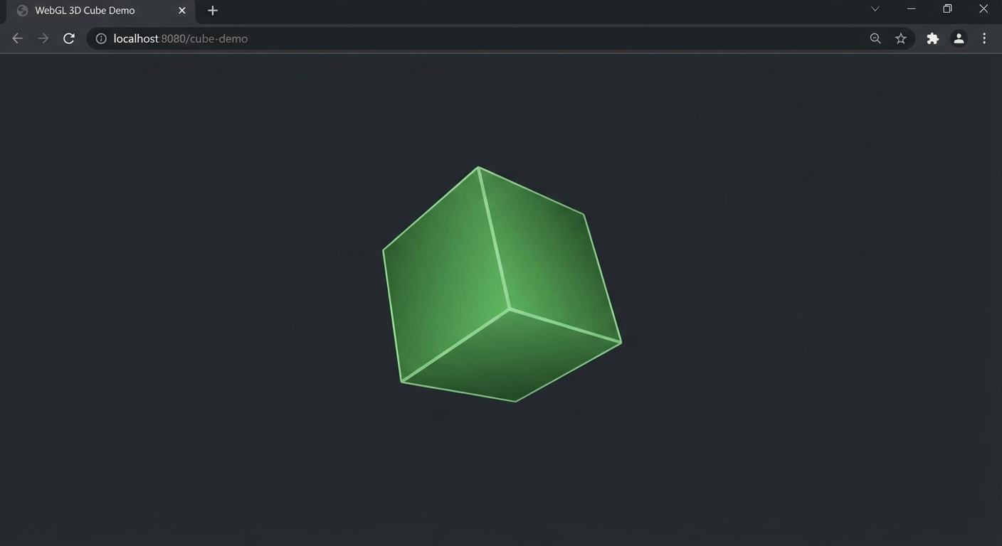
The Core Question You Are Answering
“What is the minimum set of objects and wiring needed to put a 3D shape on screen in a browser, and how does the render loop keep it alive?”
This question matters because every Three.js application – from a simple logo spinner to a AAA-quality web game – starts from this exact foundation. If you cannot set up Scene + Camera + Renderer + animation loop from memory, you will struggle to debug anything more complex. This project burns the pipeline into your muscle memory.
Concepts You Must Understand First
- The Rendering Pipeline (Scene, Camera, Renderer)
- What role does each of these three objects play, and what happens if any one of them is missing?
- Book Reference: “Computer Graphics from Scratch” by Gabriel Gambetta - Ch. 9 (Perspective Projection) and Ch. 10 (Describing and Rendering a Scene)
- BufferGeometry and Mesh
- What is the relationship between geometry (shape data) and material (appearance), and how does Mesh combine them?
- Book Reference: “Computer Graphics from Scratch” by Gabriel Gambetta - Ch. 6 (Filled Triangles)
- PerspectiveCamera Parameters
- What do FOV, aspect ratio, near plane, and far plane control, and what happens when they are wrong?
- Book Reference: “Math for Programmers” by Paul Orland - Ch. 3 (Ascending to the 3D World)
- requestAnimationFrame
- Why do we use
requestAnimationFrameinstead ofsetInterval, and what happens when the browser tab is hidden? - Reference: MDN Web Docs - requestAnimationFrame
- Why do we use
- Coordinate Systems
- Where is the origin in Three.js, which direction is “up,” and how does the camera’s position affect what you see?
- Book Reference: “Math for Programmers” by Paul Orland - Ch. 2 (Drawing with 2D Vectors) and Ch. 3 (Ascending to the 3D World)
Questions to Guide Your Design
- Canvas Setup
- How will you make the canvas fill the entire browser viewport with no scrollbars or margins?
- What CSS styles need to be applied to
<html>,<body>, and the<canvas>element?
- Camera Placement
- If the cube is at the origin (0, 0, 0), where should the camera be positioned so the cube is visible and centered?
- What FOV produces a natural-looking perspective without excessive distortion?
- Rotation Logic
- Should rotation speed be frame-rate dependent (
rotation += 0.01) or frame-rate independent (rotation += speed * delta)? - What are the consequences of each approach on a 144Hz monitor versus a 30fps mobile device?
- Should rotation speed be frame-rate dependent (
- Window Resize Handling
- What two things must be updated when the browser window resizes?
- Why must you call
camera.updateProjectionMatrix()after changing the aspect ratio?
- Module Setup
- Will you use a CDN import, npm install, or import map? What are the trade-offs for a learning project?
- How does Vite’s dev server help with ES module imports for Three.js?
Thinking Exercise
Exercise: Trace the Frame
Before writing any code, trace what happens during a single frame of the render loop on paper or a whiteboard.
Start from the moment requestAnimationFrame fires your callback:
- The browser provides a timestamp. Your
Clock.getDelta()returns 0.0167 seconds (60fps). - You increment
cube.rotation.xbyspeed * delta. - You call
renderer.render(scene, camera). - Three.js traverses the scene graph and finds one child: the cube mesh.
- Three.js reads the cube’s local matrix (built from position, rotation, scale).
- The vertex shader receives each of the cube’s 8 vertices and multiplies by modelViewMatrix * projectionMatrix.
- The GPU rasterizes the resulting 12 triangles into fragments.
- The fragment shader colors each fragment green (0x00ff00).
- The depth buffer resolves which fragments are visible (back faces behind front faces).
- The final image is written to the canvas framebuffer.
Questions to answer:
- At step 4, how many objects does Three.js find in the scene graph? What if you forgot
scene.add(cube)? - At step 6, what are the 8 vertices of a
BoxGeometry(1, 1, 1)before any transforms? - At step 9, if you used
MeshBasicMaterialwithside: THREE.DoubleSide, would the back faces also be green? - What happens if you call
renderer.render()outside ofrequestAnimationFrame– does it still work?
The Interview Questions They Will Ask
-
“What are the three objects required to render anything in Three.js, and what does each one do?”
-
“Explain the difference between
MeshBasicMaterialandMeshStandardMaterial. When would you use each?” -
“Why should you use
requestAnimationFrameinstead ofsetIntervalfor your render loop?” -
“What happens to
requestAnimationFramewhen the user switches to a different browser tab? How does this affect your animation?” -
“A user reports that your 3D cube looks stretched on their ultrawide monitor. What went wrong, and how do you fix it?”
-
“What is a draw call, and how many draw calls does a scene with a single cube require?”
Hints in Layers
Hint 1: The Starting Point
You need exactly four things before any pixels appear: a Scene, a PerspectiveCamera, a WebGLRenderer, and a function that calls renderer.render() in a loop. Create them in that order. Set the renderer’s size to window.innerWidth and window.innerHeight. Append the renderer’s DOM element (renderer.domElement) to the page.
Hint 2: Building the Cube
A Mesh is the combination of a BufferGeometry (shape) and a Material (appearance). BoxGeometry(1, 1, 1) creates a unit cube centered at the origin. MeshBasicMaterial({ color: 0x00ff00 }) gives it a flat green color with no lighting. Add the mesh to the scene with scene.add(cube). Position the camera at z = 5 so it can see the cube.
Hint 3: The Animation Loop
Create a function called animate. Inside it: (1) call requestAnimationFrame(animate) to schedule the next frame, (2) increment cube.rotation.x and cube.rotation.y by a small amount, (3) call renderer.render(scene, camera). Then call animate() once to start the loop. For frame-rate independence, use THREE.Clock and multiply rotation increments by clock.getDelta().
Hint 4: Resize Handling
Add an event listener for window.addEventListener('resize', onResize). In the onResize callback, update camera.aspect = window.innerWidth / window.innerHeight, call camera.updateProjectionMatrix(), and call renderer.setSize(window.innerWidth, window.innerHeight). Test by dragging the browser window to different sizes.
Books That Will Help
| Topic | Book | Chapter |
|---|---|---|
| Perspective projection math | “Computer Graphics from Scratch” by Gabriel Gambetta | Ch. 9 - Perspective Projection |
| Scene description and rendering | “Computer Graphics from Scratch” by Gabriel Gambetta | Ch. 10 - Describing and Rendering a Scene |
| 3D coordinate systems | “Math for Programmers” by Paul Orland | Ch. 3 - Ascending to the 3D World |
| Transformation matrices | “Math for Programmers” by Paul Orland | Ch. 5 - Computing Transformations with Matrices |
| Three.js fundamentals | “Discover Three.js” by Lewy Blue | Ch. 1 - First Steps (online, free) |
Common Pitfalls and Debugging
Problem 1: “Black screen, no cube visible”
- Why: The camera is inside the cube, or the cube is outside the camera’s frustum, or
scene.add(cube)was never called. - Fix: Set
camera.position.z = 5(move camera back). Verify the cube position is(0, 0, 0). Check thatscene.add(cube)is called before the first render. - Quick test: Log
scene.children.length– it should be 1.
Problem 2: “Cube appears but does not rotate”
- Why:
renderer.render()is called once but not inside a loop, or rotation values are not being incremented before the render call. - Fix: Ensure
requestAnimationFrame(animate)is called inside theanimatefunction, and that rotation is updated beforerenderer.render(). - Quick test: Add
console.log(cube.rotation.x)inside the loop – values should increase each frame.
Problem 3: “Cube looks stretched or squished after resizing the window”
- Why: The camera’s aspect ratio was not updated on window resize, or
updateProjectionMatrix()was not called. - Fix: In your resize handler, set
camera.aspect = window.innerWidth / window.innerHeightand callcamera.updateProjectionMatrix(). Also callrenderer.setSize(window.innerWidth, window.innerHeight). - Quick test: Resize the window and check if the cube maintains square proportions.
Problem 4: “Console shows ‘THREE is not defined’ or import errors”
- Why: Three.js is not installed or imported correctly. Common with CDN misconfigurations or missing import maps.
- Fix: If using npm:
npm install threeandimport * as THREE from 'three'. If using a CDN, ensure the import map or script tag points to a valid Three.js build. Use Vite for the simplest module setup. - Quick test: Type
THREE.REVISIONin the console – it should print the version string (e.g., “182”).
Definition of Done
- A green cube rotates continuously on both X and Y axes on a black background
- The canvas fills the entire browser viewport with no scrollbars
- Resizing the browser window updates the aspect ratio without distortion
- Switching to another tab and back does not break the animation
- The console shows zero errors and zero warnings
renderer.info.render.callsequals 1renderer.info.render.trianglesequals 12- Code uses
requestAnimationFrame, notsetIntervalorsetTimeout - Frame-rate independent rotation is implemented using
Clock.getDelta()
Project 2: A Solar System Mobile
- File: P02-solar-system-mobile.md
- Main Programming Language: JavaScript
- Alternative Programming Languages: TypeScript, Kotlin/JS, ClojureScript
- Coolness Level: 3 - “That’s actually cool” (visually engaging, shows mastery of a concept)
- Business Potential: 1 - Resume / Portfolio Only
- Difficulty: Intermediate - Guided Exploration (some ambiguity, multiple valid approaches)
- Knowledge Area: Scene Graphs / Transformations / Hierarchical Animation
- Software or Tool: Three.js, Vite, lil-gui (for parameter tweaking)
- Main Book: “Math for Programmers” by Paul Orland - Ch. 4 (Transforming Vectors and Graphics) and Ch. 5 (Computing Transformations with Matrices)
What you will build: An animated solar system with a yellow emissive sun at the center, a blue-green planet orbiting the sun, and a gray moon orbiting the planet – all with different orbital speeds, powered by a scene graph hierarchy that makes parent-child transformations do the heavy lifting.
Why it teaches Three.js: The scene graph is the backbone of every non-trivial 3D application. Without understanding parent-child relationships and how transformations cascade, you cannot build articulated characters, vehicle assemblies, robotic arms, UI panels attached to 3D objects, or any system where objects move relative to each other. This project makes the scene graph visceral: the moon orbits the planet because it is a child of the planet’s orbital group – move the planet and the moon follows for free.
Core challenges you will face:
- Building a scene graph hierarchy -> Maps to Object3D parent-child relationships and Groups
- Separating orbital motion from self-rotation -> Maps to local vs world space transforms
- Getting emissive materials right -> Maps to MeshBasicMaterial emissive properties and MeshStandardMaterial
- Coordinating multiple animation speeds -> Maps to animation loop with delta time and elapsed time
Real World Outcome
When you open the page in a browser:
Initial View:
The scene opens with the camera pulled back far enough to see the entire orbital system. The background is black (the void of space). At the center sits a large yellow sphere – the sun. It glows uniformly because it uses MeshBasicMaterial with a warm yellow-orange color (#ffcc00), making it appear self-luminous since basic materials ignore lighting. The sun is roughly 3x the diameter of the planet.
The Planet:
A blue-green sphere (color: #2266aa or similar ocean blue-green) orbits the sun at a radius of approximately 10 units. It completes one full orbit every 10 seconds. The planet uses MeshStandardMaterial with a roughness of 0.7 and metalness of 0.1, so it responds to light. The side of the planet facing the sun is brightly lit; the far side is dark. The planet also rotates on its own axis (self-rotation), completing one self-rotation every 3 seconds, so you can see the lit/dark terminator shift across its surface.
The Moon:
A smaller gray sphere (color: #888888) orbits the planet at a radius of approximately 3 units from the planet’s center. It completes one orbit around the planet every 4 seconds. The moon is roughly 0.3x the diameter of the planet. It also uses MeshStandardMaterial and is lit by the same light source (a PointLight placed at the sun’s position), so it shows light/dark sides.
Lighting:
A PointLight is placed at the sun’s position (0, 0, 0) with an intensity of 2.0 and a warm white color. This creates a single light source that illuminates both the planet and moon from the center of the system. An AmbientLight with very low intensity (0.05) provides minimal fill so the dark sides of objects are not completely invisible.
Key Visual Test: Watch the moon for 30 seconds. It orbits the planet while the planet simultaneously orbits the sun. The moon traces a complex path through world space (an epicycloid), but your code only specifies the moon’s rotation around the planet – the sun-orbit comes for free because the moon is a child of the planet’s orbital group. This is the scene graph at work.
Console Verification:
scene.childrenincludes the sun mesh, aGroupfor the planet orbit, and lights- The planet orbit Group contains the planet mesh and a second
Groupfor the moon orbit - The moon orbit Group contains the moon mesh
renderer.info.render.callsequals 3 (sun, planet, moon)
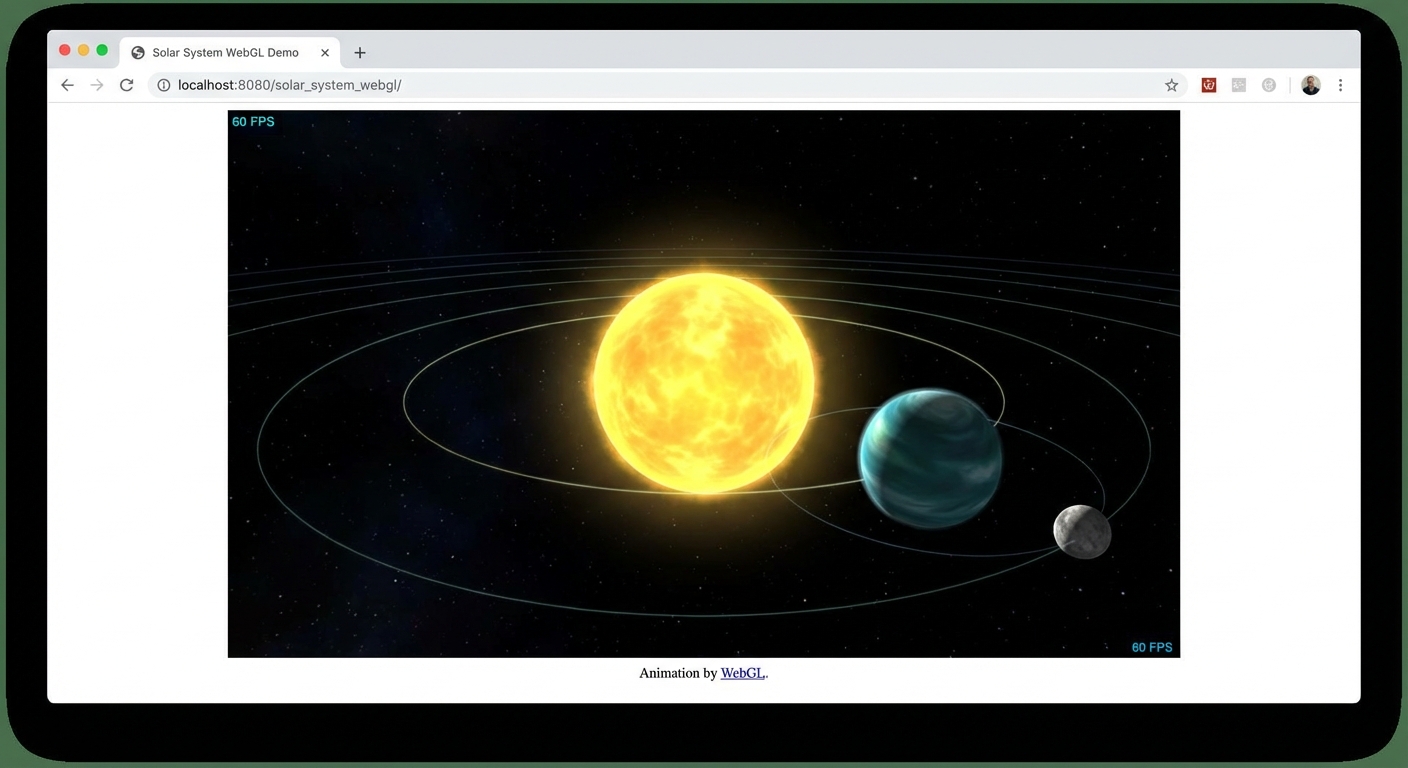
The Core Question You Are Answering
“How does a scene graph hierarchy make complex multi-body motion trivial, and what is the difference between local space and world space?”
This question matters because almost every real Three.js application involves objects that move relative to other objects: a character’s hand relative to their arm, a car’s wheel relative to its body, a tooltip relative to a 3D object. The scene graph is how Three.js manages these relationships, and if you do not understand it, you will end up writing brittle code that manually calculates world positions for every object every frame.
Concepts You Must Understand First
- Scene Graph and Object3D Hierarchy
- What happens to a child object’s position when its parent moves? How is
matrixWorldcomputed? - Book Reference: “Math for Programmers” by Paul Orland - Ch. 5 (Computing Transformations with Matrices)
- What happens to a child object’s position when its parent moves? How is
- Local Space vs World Space
- If the moon’s local position is
(3, 0, 0)and its parent (planet orbital group) is at(10, 0, 0), where is the moon in world space? - Book Reference: “Math for Programmers” by Paul Orland - Ch. 4 (Transforming Vectors and Graphics)
- If the moon’s local position is
- Group vs Object3D
- When should you use a
Groupas an invisible pivot point versus placing objects directly in the scene? - Reference: Three.js docs - Group, Object3D
- When should you use a
- Emissive Materials vs Lit Materials
- Why does the sun use
MeshBasicMaterial(ignores lights, always full brightness) while the planet usesMeshStandardMaterial(responds to lights)? - Reference: Discover Three.js - Materials chapter
- Why does the sun use
- PointLight and Light Attenuation
- How does a
PointLightilluminate objects at different distances, and what parameters control its falloff? - Book Reference: “Computer Graphics from Scratch” by Gabriel Gambetta - Ch. 3 (Light)
- How does a
- Trigonometric Orbits
- How do sine and cosine produce circular motion, and how does
elapsedTimedrive a continuous orbit? - Book Reference: “Math for Programmers” by Paul Orland - Ch. 2 (Drawing with 2D Vectors, polar coordinates)
- How do sine and cosine produce circular motion, and how does
Questions to Guide Your Design
- Hierarchy Design
- Should the planet be a direct child of the scene, or a child of an intermediate Group that handles orbital rotation?
- If you want the planet to orbit AND self-rotate, why do you need a separate Group for the orbit?
- Orbital Mechanics
- Will you drive orbits by directly setting
x = radius * cos(time)andz = radius * sin(time), or by rotating a parent Group? - What is the advantage of rotating a parent Group with the planet offset on the X axis?
- Will you drive orbits by directly setting
- Light Placement
- Should the PointLight be a child of the sun mesh, or placed independently at the same position?
- What happens if the light’s distance/decay are not configured properly?
- Scale and Proportions
- What radii and orbital distances look good on screen? How do you avoid the moon being too small to see or the planet obscuring the sun?
- Should you use realistic proportions (the real Earth is tiny compared to the sun) or artistic proportions?
- Animation Timing
- How will you make each body orbit at a different speed while using the same animation loop?
- Should you use
Clock.getElapsedTime()orClock.getDelta()for continuous orbital motion?
Thinking Exercise
Exercise: Draw the Scene Graph Tree
On paper, draw a tree diagram showing every Object3D in your scene and its parent-child relationships. Include:
Scene
 |-- AmbientLight
 |-- PointLight (at sun position)
 |-- Sun (Mesh: SphereGeometry + MeshBasicMaterial, yellow)
 |-- PlanetOrbitGroup (Group: rotation.y drives orbit)
      |-- Planet (Mesh: SphereGeometry + MeshStandardMaterial, blue-green)
      |    position: (10, 0, 0) relative to PlanetOrbitGroup
      |-- MoonOrbitGroup (Group: rotation.y drives moon orbit)
           |    position: (10, 0, 0) relative to PlanetOrbitGroup
           |-- Moon (Mesh: SphereGeometry + MeshStandardMaterial, gray)
                position: (3, 0, 0) relative to MoonOrbitGroup
Now trace what happens when PlanetOrbitGroup.rotation.y increments by 0.1 radians:
Questions to answer:
- Does the sun move? (No – it is not a child of PlanetOrbitGroup)
- Where does the planet end up in world space? (It traces a circle of radius 10 around the origin)
- Where does the moon end up in world space? (Its world position combines the planet orbit and its own orbit)
- If you set
MoonOrbitGroup.rotation.yto a different speed, does the moon orbit the planet independently? (Yes)
The Interview Questions They Will Ask
-
“Explain the Three.js scene graph. How do parent-child transforms work?”
-
“What is the difference between an object’s
position(local space) andgetWorldPosition()(world space)?” -
“Why would you use an empty
Groupas a parent for a mesh instead of placing the mesh directly in the scene?” -
“If you want an object to orbit a point, what are two different approaches – one using trigonometry directly and one using the scene graph?”
-
“What is gimbal lock, and how does it relate to Euler rotation order in Three.js?”
-
“You have a robotic arm with a shoulder, elbow, and wrist joint. How would you structure the scene graph so that rotating the shoulder moves the entire arm?”
Hints in Layers
Hint 1: The Hierarchy Approach
Create two Group objects: planetOrbitGroup and moonOrbitGroup. Add the planet mesh as a child of planetOrbitGroup, offset it along the X axis. Add moonOrbitGroup as a sibling of the planet inside planetOrbitGroup, also offset on X. Add the moon mesh as a child of moonOrbitGroup, offset further. Rotating planetOrbitGroup.rotation.y orbits everything around the sun. Rotating moonOrbitGroup.rotation.y orbits only the moon around the planet.
Hint 2: Making the Sun Glow
Use MeshBasicMaterial({ color: 0xffcc00 }) for the sun. Basic materials are unaffected by lights, so the sun appears uniformly bright from all angles, simulating self-illumination. Place a PointLight at the same position as the sun to illuminate other objects. Set the light’s intensity to 2 or higher and optionally set decay to 1 for realistic falloff.
Hint 3: Driving the Animation
In the animation loop, use clock.getElapsedTime() (not getDelta()) for orbital rotation. Set planetOrbitGroup.rotation.y = elapsed * 0.5 for a smooth 0.5 rad/s orbit. Set moonOrbitGroup.rotation.y = elapsed * 1.5 for a faster moon orbit. For self-rotation, use planet.rotation.y = elapsed * 2.0. Using getElapsedTime() gives absolute angles that produce smooth, continuous orbits without accumulation drift.
Hint 4: Debugging the Hierarchy
If the moon is orbiting the sun instead of the planet, your hierarchy is wrong. Check that moonOrbitGroup is a child of planetOrbitGroup, not the scene. Use scene.traverse((obj) => console.log(obj.type, obj.parent?.type)) to print the hierarchy. Alternatively, add AxesHelper to each group to visualize their local coordinate axes.
Books That Will Help
| Topic | Book | Chapter |
|---|---|---|
| Vector transformations | “Math for Programmers” by Paul Orland | Ch. 4 - Transforming Vectors and Graphics |
| Matrix multiplication for transforms | “Math for Programmers” by Paul Orland | Ch. 5 - Computing Transformations with Matrices |
| Lighting and illumination | “Computer Graphics from Scratch” by Gabriel Gambetta | Ch. 3 - Light |
| Scene description | “Computer Graphics from Scratch” by Gabriel Gambetta | Ch. 10 - Describing and Rendering a Scene |
| Scene graph fundamentals | “Discover Three.js” by Lewy Blue | Transformations chapter (online) |
Common Pitfalls and Debugging
Problem 1: “Moon orbits the sun instead of the planet”
- Why: The moon or its orbit group was added as a child of the scene (or the sun) instead of the planet’s orbit group.
- Fix: Ensure the hierarchy is: Scene -> PlanetOrbitGroup -> MoonOrbitGroup -> Moon. The moon orbit group must be a child of the planet orbit group.
- Quick test:
moonOrbitGroup.parent === planetOrbitGroupshould betrue.
Problem 2: “Planet and moon are completely black”
- Why: No light source in the scene, or the light is at the wrong position, or the objects use
MeshStandardMaterialbut there is no light to illuminate them. - Fix: Add a
PointLightat the sun’s position with sufficient intensity (at least 1.0). Add a dimAmbientLight(intensity 0.05) so dark sides are not pure black. - Quick test: Temporarily switch the planet’s material to
MeshBasicMaterial– if it becomes visible, the issue is lighting.
Problem 3: “Orbit looks elliptical instead of circular”
- Why: The camera’s aspect ratio is wrong, or the planet is not offset purely along the X axis (it has a Y or Z offset that creates a diagonal path).
- Fix: Verify the planet’s position is
(10, 0, 0)in its parent’s local space. Ensure the orbit group only rotates around Y. Check the camera aspect ratio matches the window dimensions. - Quick test: View the scene from directly above (camera at Y = 50, looking down) to verify the orbit path is circular.
Problem 4: “Self-rotation and orbital rotation are fighting each other”
- Why: You are applying both self-rotation and orbital rotation to the same object. Self-rotation should be on the mesh; orbital rotation should be on the parent Group.
- Fix: Rotate the mesh itself for self-spin (
planet.rotation.y += ...). Rotate the parent Group for orbit (planetOrbitGroup.rotation.y += ...). These are independent transforms at different levels of the hierarchy. - Quick test: Comment out the orbital rotation. Does the planet still spin in place? If yes, self-rotation is correct.
Definition of Done
- Sun is a yellow sphere at the center that appears self-luminous (unlit material)
- Planet orbits the sun in a circular path with smooth, continuous motion
- Moon orbits the planet (not the sun) in a separate circular path
- Planet and moon respond to lighting (lit side vs dark side is visible)
- All three bodies have visually distinct sizes (sun > planet > moon)
- Orbital speeds are different for planet and moon
- Planet self-rotates independently of its orbital motion
- Scene graph hierarchy is correct: Scene -> PlanetOrbitGroup -> (Planet, MoonOrbitGroup -> Moon)
- Animation uses
getElapsedTime()for smooth, continuous orbits - Resizing the browser window does not break proportions
Project 3: Textured Earth and Moon
- File: P03-textured-earth-moon.md
- Main Programming Language: JavaScript
- Alternative Programming Languages: TypeScript, Elm (via ports), PureScript
- Coolness Level: 3 - “That’s actually cool” (visually impressive, photorealistic look)
- Business Potential: 1 - Resume / Portfolio Only
- Difficulty: Intermediate - Guided Exploration (texture loading, PBR materials, shadow setup)
- Knowledge Area: Materials / Texturing / Lighting / Shadows
- Software or Tool: Three.js, Vite, NASA Blue Marble textures, lil-gui
- Main Book: “Computer Graphics from Scratch” by Gabriel Gambetta - Ch. 14 (Textures)
What you will build: A photorealistic 3D Earth with NASA satellite textures (daytime color map, cloud layer, specular ocean map) and a cratered Moon, both lit by a single directional “sun” light that produces realistic lighting with light glinting off the oceans and shadows cast by the Moon.
Why it teaches Three.js: Textures transform flat-shaded geometry into photorealistic surfaces. Understanding how textures load, how UV coordinates map 2D images onto 3D shapes, and how PBR material channels (color, roughness, metalness, normal, specular) combine is essential for any production Three.js work – from product configurators to architectural visualizations. This project forces you to work with multiple texture maps on a single material and see how each channel affects the final appearance.
Core challenges you will face:
- Loading and applying multiple texture maps -> Maps to TextureLoader, async loading patterns, and material channels
- Understanding UV mapping on a sphere -> Maps to UV coordinates and how equirectangular textures wrap around SphereGeometry
- Configuring PBR material properties -> Maps to MeshStandardMaterial roughness, metalness, and map channels
- Setting up realistic lighting with shadows -> Maps to DirectionalLight, shadow mapping, and shadow camera configuration
Real World Outcome
When you open the page in a browser:
Loading Phase (1-3 seconds): A black background appears while textures load. Optionally, a simple loading indicator or progress bar shows the status of texture downloads (the Earth textures alone are several megabytes).
Earth Appearance: A sphere fills roughly 40% of the viewport width. Its surface displays the NASA Blue Marble texture – you see recognizable continents, oceans, ice caps, and land masses in full color. The texture wraps seamlessly around the sphere with no visible seam at the antimeridian (180 degrees longitude). The Earth rotates slowly on its axis (one full rotation every 15-20 seconds).
Material Detail: The Earth has multiple texture channels working together:
- Color/Albedo Map: The daytime satellite image from NASA showing land, ocean, and ice
- Specular Map (or roughnessMap): Oceans have low roughness (shiny, reflective) while land has high roughness (matte). As the Earth rotates, you see a bright specular highlight gliding across the ocean surfaces – light glinting off the water – while continents remain diffuse
- Cloud Layer: A semi-transparent cloud texture applied to a slightly larger sphere nested just outside the Earth surface. The clouds rotate at a different speed than the Earth, creating realistic atmospheric motion
- Optional Normal Map: Subtle surface relief giving mountain ranges and terrain a 3D appearance without adding geometry
Moon Appearance:
A smaller gray sphere (roughly 1/4 the Earth’s diameter) is positioned to the upper-right of the Earth. It displays a crater texture with visible maria (dark regions) and highland areas. The Moon uses MeshStandardMaterial with moderate roughness (0.9) and no specular highlights – its surface is uniformly matte.
Lighting:
A single DirectionalLight simulates sunlight, coming from the left side of the screen. The Earth and Moon show a clear bright side and dark side. The terminator (line between day and night) is visible. The dark side is not pitch black thanks to a dim AmbientLight (intensity ~0.06). On the bright side, ocean surfaces catch specular highlights.
Shadow (Optional Advanced): The Moon casts a faint shadow on the Earth’s surface when it passes between the light source and the Earth (simulating an eclipse). The shadow is soft and circular on the Earth’s curved surface.
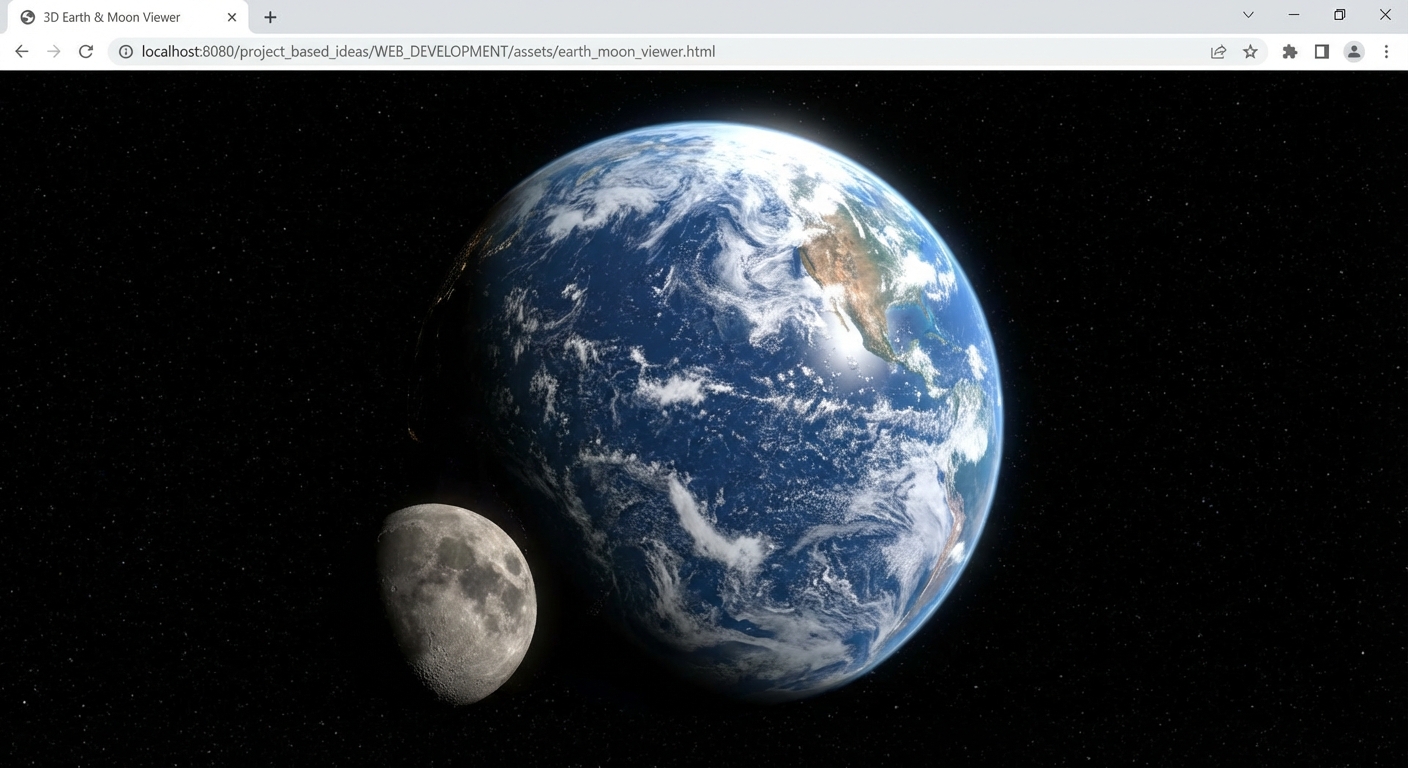
The Core Question You Are Answering
“How do multiple texture maps combine on a single PBR material to create surfaces that look photorealistic, and what role does each map channel play?”
This matters because professional 3D content uses 4-8 texture maps per material: color, normal, roughness, metalness, ambient occlusion, displacement, emissive. Understanding how these channels interact is the difference between “obviously CG” and “wait, is that a photograph?”
Concepts You Must Understand First
- TextureLoader and Async Loading
- How does Three.js load image files into GPU textures, and what happens if you try to render before loading completes?
- Reference: Three.js docs - TextureLoader, LoadingManager
- UV Mapping on Built-in Geometries
- How does
SphereGeometrymap UV coordinates so that an equirectangular texture wraps around the sphere correctly? - Book Reference: “Computer Graphics from Scratch” by Gabriel Gambetta - Ch. 14 (Textures)
- How does
- PBR Material Channels
- What does each map channel (map, roughnessMap, metalnessMap, normalMap, aoMap) control, and how do they interact?
- Reference: Three.js docs - MeshStandardMaterial
- Specular Highlights on Water
- Why do oceans appear shiny and land appears matte? How does a specular/roughness map encode this per-pixel?
- Book Reference: “Computer Graphics from Scratch” by Gabriel Gambetta - Ch. 13 (Shading)
- Shadow Mapping
- How does Three.js render the scene from the light’s perspective to create a depth map, and how is that map used to determine which fragments are in shadow?
- Reference: Three.js Journey - Shadows lesson
Questions to Guide Your Design
- Texture Sourcing
- Where will you download the NASA Blue Marble textures? What resolution is appropriate (2K, 4K, 8K)?
- Do you need separate downloads for the color map, cloud map, specular map, and normal map?
- Cloud Layer Technique
- How do you render clouds as a separate semi-transparent layer above the Earth surface?
- Should the cloud sphere be a separate mesh with its own material, or a second texture on the same material?
- Specular Map Workflow
- How do you convert a specular map (white = shiny, black = matte) into a roughness map (white = rough, black = smooth) for MeshStandardMaterial?
- Can you invert the specular map, or should you use it as-is with the
roughnessMapchannel?
- Lighting for Realism
- What angle should the directional light come from to show the most visually interesting terminator on the Earth?
- How do you configure shadow mapping for the directional light to produce a clean shadow?
- Texture Color Space
- Which textures should use sRGB encoding (color maps) and which should use linear encoding (normal maps, roughness maps)?
- What happens if you use the wrong color space for a normal map?
Thinking Exercise
Exercise: Map the Material Channels
Draw a diagram of MeshStandardMaterial showing all the map channels you will use for the Earth. For each channel, describe what the texture looks like and what it controls:
MeshStandardMaterial
  |
  |-- map (color):       NASA Blue Marble image
  |                      -> Controls base color (albedo) at every pixel
  |
  |-- roughnessMap:      Inverted specular map (or dedicated roughness)
  |                      -> White pixels = rough (land), Black = smooth (ocean)
  |                      -> Controls how scattered vs sharp reflections are
  |
  |-- normalMap:         Terrain relief texture (blue-purple image)
  |                      -> Fakes surface bumps without geometry
  |                      -> Each RGB pixel encodes a surface normal direction
  |
  |-- metalnessMap:      Probably not used (Earth is not metallic)
  |                      -> Could set metalness to 0 globally
  |
  |-- emissiveMap:       Night lights texture (optional, advanced)
  |                      -> City lights visible on the dark side
Questions to answer:
- If you swap the roughnessMap for the normalMap by accident, what would the Earth look like?
- Why is the normalMap predominantly blue in color? What do the R, G, and B channels represent?
- If you set
metalness: 1.0on the entire Earth, what would happen to the oceans?
The Interview Questions They Will Ask
-
“What is the difference between a normal map and a displacement map? When would you use each?”
-
“Explain what roughness and metalness control in a PBR material. What happens at the extremes (0 and 1)?”
-
“Why should texture dimensions be powers of 2 (512, 1024, 2048)? What happens with non-power-of-2 textures?”
-
“How does shadow mapping work? Describe the process of rendering a shadow map and using it during the main render pass.”
-
“What is the difference between sRGB and linear color space, and why does it matter for texture loading in Three.js?”
-
“A user reports that their normal map makes the surface look metallic and wrong. What likely happened?”
Hints in Layers
Hint 1: Texture Loading Pattern
Create a TextureLoader instance. Load each texture with loader.load('path/to/texture.jpg'). Store the returned texture objects and assign them to the appropriate material properties: map for color, roughnessMap for roughness, normalMap for normals. Use a LoadingManager to track when all textures are loaded before showing the scene.
Hint 2: Cloud Layer as Separate Mesh
Create a second SphereGeometry with a radius 0.5-1% larger than the Earth. Apply the cloud texture as the map on a MeshStandardMaterial with transparent: true and opacity: 0.4. The black areas of the cloud texture become transparent; white areas become clouds. Rotate this sphere at a slightly different speed than the Earth for realism.
Hint 3: Specular Oceans
NASA provides a specular map where oceans are white and land is black. Three.js’s MeshStandardMaterial uses roughnessMap where white = rough. Since the NASA map is inverted (white = shiny oceans), you either need to invert the image in an editor before loading, or set the base roughness to 1.0 and the material will combine the base value with the map. Alternatively, use the specular map directly and adjust the base roughness until oceans appear shiny.
Hint 4: Shadow Configuration
Enable shadows: renderer.shadowMap.enabled = true, renderer.shadowMap.type = THREE.PCFSoftShadowMap. On the directional light: light.castShadow = true, light.shadow.mapSize.set(2048, 2048). On the moon: moon.castShadow = true. On the Earth: earth.receiveShadow = true. Adjust light.shadow.camera.left/right/top/bottom to tightly frame the scene for maximum shadow resolution.
Books That Will Help
| Topic | Book | Chapter |
|---|---|---|
| Texture mapping fundamentals | “Computer Graphics from Scratch” by Gabriel Gambetta | Ch. 14 - Textures |
| Shading and illumination | “Computer Graphics from Scratch” by Gabriel Gambetta | Ch. 13 - Shading |
| Shadows and reflections | “Computer Graphics from Scratch” by Gabriel Gambetta | Ch. 4 - Shadows and Reflections |
| 3D coordinate math | “Math for Programmers” by Paul Orland | Ch. 3 - Ascending to the 3D World |
| PBR materials (advanced) | “Real-Time Rendering” by Akenine-Moller et al. | Ch. 4 - Visual Appearance |
Common Pitfalls and Debugging
Problem 1: “Earth is black or untextured despite loading the texture”
- Why: The texture has not finished loading when the first render occurs, or the file path is incorrect, or the texture’s color space is not set correctly.
- Fix: Use
LoadingManagerorloader.load(url, onLoadCallback)to ensure textures are loaded before rendering. Check the browser Network tab to verify the file is being fetched. Settexture.colorSpace = THREE.SRGBColorSpacefor color maps. - Quick test: Replace the texture with
MeshBasicMaterial({ color: 0xff0000 })– if the sphere is now visible, the issue is texture loading.
Problem 2: “Visible seam line on the sphere at one longitude”
- Why: The equirectangular texture has a slight mismatch at the edges where U=0 wraps to U=1. Some NASA textures do not tile perfectly, or the UV seam on
SphereGeometrycreates a visible artifact. - Fix: Use higher resolution textures where the seam is less visible. Ensure
texture.wrapS = THREE.RepeatWrapping. For the cloud layer, this is usually not noticeable. - Quick test: Rotate the Earth so the seam faces the camera. If there is a visible line, the texture edges do not match.
Problem 3: “Normal map makes the surface look completely wrong – metallic or inverted”
- Why: The normal map’s color space is set to sRGB instead of linear, or the normal map is in a different tangent-space convention than Three.js expects.
- Fix: Set
normalMap.colorSpace = THREE.LinearSRGBColorSpace(data textures must use linear). Try settingmaterial.normalScale = new THREE.Vector2(1, -1)to flip the green channel if normals appear inverted. - Quick test: Remove the normalMap temporarily. If the surface looks correct without it, the normalMap settings are the issue.
Problem 4: “Shadows are not appearing”
- Why: One of the many shadow setup steps was missed. Shadows require:
renderer.shadowMap.enabled,light.castShadow,mesh.castShadow,mesh.receiveShadow, and a properly configured shadow camera. - Fix: Go through the checklist: (1) renderer, (2) light, (3) casting mesh, (4) receiving mesh, (5) shadow camera bounds. All five must be correctly configured.
- Quick test: Set
light.shadow.camera.near = 0.1,far = 100, and make the left/right/top/bottom values large enough to encompass both the moon and Earth.
Definition of Done
- Earth displays NASA Blue Marble texture with recognizable continents and oceans
- Oceans show specular highlights (light glinting) while land remains matte
- Cloud layer is visible as a semi-transparent overlay that rotates independently
- Moon displays a crater texture and has a matte, gray appearance
- Single directional light creates a clear day/night terminator on both Earth and Moon
- Dark sides are faintly visible (ambient light present)
- Earth rotates on its axis with smooth animation
- Textures use correct color spaces (sRGB for color, linear for normal/roughness)
- No texture loading errors in the console
- Browser resize maintains correct proportions
Project 4: Interactive Museum
- File: P04-interactive-museum.md
- Main Programming Language: JavaScript
- Alternative Programming Languages: TypeScript, Svelte + Three.js, React Three Fiber
- Coolness Level: 3 - “That’s actually cool” (interactive, explorable 3D environment)
- Business Potential: 2 - Freelance Ready / Small Business Value
- Difficulty: Intermediate - Guided Exploration (raycasting, controls, DOM/3D integration)
- Knowledge Area: Interactivity / Raycasting / Camera Controls / DOM-3D Integration
- Software or Tool: Three.js, OrbitControls, Vite, lil-gui
- Main Book: “Computer Graphics from Scratch” by Gabriel Gambetta - Ch. 9 (Perspective Projection)
What you will build: A 3D museum room with pedestals displaying geometric objects. The user orbits the camera with the mouse, hovers over objects to highlight them, and clicks to select objects and display an information panel. This is the first project where user interaction drives the experience.
Why it teaches Three.js: Real Three.js applications are interactive – users click, hover, drag, and explore. Raycasting (casting an invisible ray from the camera through the mouse cursor into the 3D scene) is the fundamental technique for 3D mouse interaction. This project teaches you how to convert 2D screen coordinates to 3D space, detect which object the user is pointing at, and respond with visual feedback and DOM UI updates. These skills are directly applicable to product configurators, data visualizations, and any 3D UI.
Core challenges you will face:
- Converting mouse coordinates to Normalized Device Coordinates (NDC) -> Maps to screen-to-3D coordinate conversion
- Using Raycaster to detect hover and click targets -> Maps to ray-object intersection testing
- Providing visual feedback (highlight, glow) -> Maps to dynamic material property changes
- Integrating HTML/DOM UI with 3D scene -> Maps to hybrid 2D/3D application architecture
Real World Outcome
When you open the page in a browser:
The Room: A simple rectangular room fills the viewport. The floor is a large plane with a subtle checkerboard or wood texture. The walls are light gray. The ceiling has a slight ambient illumination. The room is approximately 20x20 units, giving enough space for the camera to orbit without clipping through walls.
The Pedestals and Objects: Five pedestals (white boxes, roughly 0.5 x 1 x 0.5 units) are arranged in a semi-circle or grid pattern on the floor. On top of each pedestal sits a different geometric object:
- A red dodecahedron
- A blue torus knot
- A green icosahedron
- A purple torus
- An orange octahedron
Each object uses MeshStandardMaterial with moderate metalness (0.3) and low roughness (0.4), making them slightly reflective and visually interesting.
Camera Interaction:
OrbitControls is enabled. The user can:
- Left-click drag: Orbit the camera around the center of the room
- Scroll wheel: Zoom in and out
- Right-click drag: Pan the camera sideways
- The camera is constrained so it cannot go below the floor or too far from the room
Hover Behavior: When the mouse cursor hovers over one of the five display objects, the following happens within 1 frame:
- The cursor changes to a pointer (
cursor: pointer) - The hovered object’s emissive color changes to a soft glow (e.g., emissive: 0x333333), making it appear subtly illuminated
- The object scales up slightly (1.0 -> 1.1) with a smooth transition
- When the mouse moves away, the object returns to its normal state within 1 frame
Click Behavior: When the user clicks on a display object:
- The object’s emissive color changes to a brighter glow (emissive: 0x666600), indicating selection
- A DOM-based information panel slides in from the right side of the screen (or appears as an overlay)
- The panel displays: the object’s name, a description of the geometry type, the number of faces, and a “Close” button
- Clicking a different object updates the panel content
- Clicking the “Close” button or clicking empty space dismisses the panel
- The previously selected object’s glow fades when deselected
Lighting: Two or three lights illuminate the room:
- A
HemisphereLightfor ambient fill (sky: warm white, ground: cool gray) - Two
SpotLights angled from above to create dramatic shadows from the pedestals - The room has visible cast shadows from the objects and pedestals
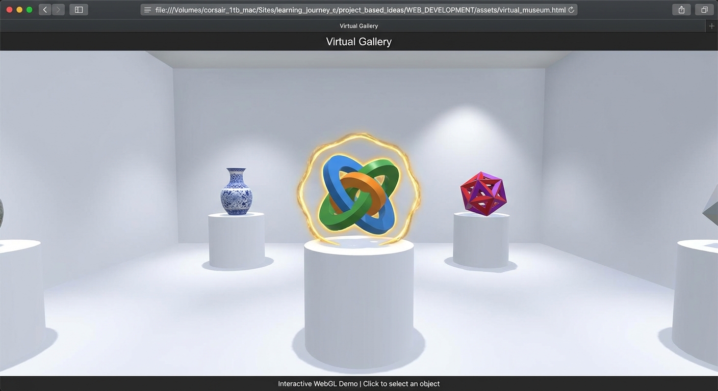
The Core Question You Are Answering
“How do you determine which 3D object is under the user’s mouse cursor, and how do you build interactive 3D experiences that respond to hover, click, and selection?”
This matters because 90% of commercial Three.js applications require user interaction. Product configurators need click-to-select-part. Data visualizations need hover-to-show-tooltip. Games need click-to-attack. Raycasting is the bridge between the 2D screen and the 3D world.
Concepts You Must Understand First
- Raycaster and Ray-Object Intersection
- How does
Raycaster.setFromCamera(mouse, camera)create a ray, and what doesintersectObjects()return? - Reference: Three.js docs - Raycaster
- How does
- Normalized Device Coordinates (NDC)
- What is the NDC coordinate system, and how do you convert
event.clientX/clientYto NDC? - Book Reference: “Computer Graphics from Scratch” by Gabriel Gambetta - Ch. 9 (Perspective Projection, viewport mapping)
- What is the NDC coordinate system, and how do you convert
- OrbitControls
- How does OrbitControls manage camera position, and what events does it consume that might conflict with your click/hover handling?
- Reference: Three.js docs - OrbitControls
- Emissive Material Properties
- How does the emissive property on MeshStandardMaterial add self-illumination without affecting lighting calculations?
- Reference: Three.js docs - MeshStandardMaterial.emissive
- DOM/Canvas Integration
- How do you layer HTML elements on top of the Three.js canvas for UI panels and tooltips?
- Reference: CSS
position: absolute+pointer-eventsmanagement
Questions to Guide Your Design
- Raycasting Strategy
- Should you raycast on
mousemove(every pixel of mouse movement) or throttle it to once per frame in the animation loop? - How do you avoid raycasting against every object in the scene? Should you maintain a separate array of “interactive” objects?
- Should you raycast on
- Highlight Feedback
- Should you modify the object’s existing material (change emissive) or swap to a different material on hover?
- What is the performance implication of creating new materials on every hover event?
- Selection State Management
- How do you track which object is currently selected? What data structure holds the selection state?
- When a new object is selected, how do you deselect the previous one?
- DOM Panel Positioning
- Should the info panel be a fixed position DOM element overlaying the canvas, or should you use CSS3DRenderer to place it in 3D space?
- How do you ensure mouse events on the DOM panel do not trigger raycasting on the 3D scene behind it?
- Controls Conflict
- OrbitControls uses left-click for orbiting. How do you distinguish between “click to select an object” and “click-drag to orbit”?
- Should you use
pointerdown+pointerupwith a distance threshold to detect clicks vs drags?
Thinking Exercise
Exercise: Trace the Raycast
Imagine the user clicks at pixel (960, 540) on a 1920x1080 canvas. Trace the raycast step by step:
- Convert to NDC:
mouse.x = (960 / 1920) * 2 - 1 = 0.0,mouse.y = -(540 / 1080) * 2 + 1 = 0.0. The mouse is at the center of the screen. raycaster.setFromCamera({x: 0, y: 0}, camera)creates a ray from the camera’s position, pointing directly forward through the center of the viewport.raycaster.intersectObjects(interactiveObjects)tests this ray against each object’s bounding sphere for a quick check, then against the actual triangles for hits.- The result is an array sorted by distance:
[{distance: 5.2, object: torus, point: Vector3(...)}, {distance: 8.1, object: pedestal, point: Vector3(...)}] - You take
intersects[0].object(the torus at distance 5.2) as the clicked object.
Questions to answer:
- What happens if the mouse is at (0, 0) in screen pixels? What are the NDC coordinates? (-1, 1) – the top-left corner of the screen.
- If the canvas has a CSS margin of 100px on the left, does the standard NDC formula still work? No – you need
canvas.getBoundingClientRect()to account for the offset. - If two objects overlap from the camera’s perspective, which one does
intersects[0]return? The closest one (lowest distance).
The Interview Questions They Will Ask
-
“How does raycasting work in Three.js? Walk me through the process from mouse click to detecting the clicked object.”
-
“What are Normalized Device Coordinates, and why do you need to convert screen coordinates to NDC for raycasting?”
-
“How would you implement a hover highlight effect on 3D objects without creating new materials every frame?”
-
“You have a 3D scene with 10,000 objects, but only 50 are interactive. How do you optimize raycasting performance?”
-
“How do you handle the conflict between OrbitControls (which uses mouse click for orbit) and click-to-select on 3D objects?”
-
“Describe two approaches for displaying information about a clicked 3D object: DOM overlay vs CSS3DRenderer. What are the trade-offs?”
Hints in Layers
Hint 1: Setting Up the Raycaster
Create a Raycaster and a Vector2 for the mouse position. Add a pointermove event listener on the canvas that updates the mouse Vector2 using NDC conversion: mouse.x = (event.clientX / window.innerWidth) * 2 - 1; mouse.y = -(event.clientY / window.innerHeight) * 2 + 1. In the animation loop, call raycaster.setFromCamera(mouse, camera) and then raycaster.intersectObjects(interactiveObjects).
Hint 2: Hover Highlight
Maintain a variable hoveredObject = null. In the animation loop after raycasting: if intersects has results, set hoveredObject = intersects[0].object and change its material.emissive.set(0x333333). If the previous hoveredObject is different from the current, reset its emissive to black. Update the cursor style: document.body.style.cursor = hoveredObject ? 'pointer' : 'default'.
Hint 3: Click vs Drag Detection
Listen for pointerdown and pointerup. On pointerdown, store the mouse position and timestamp. On pointerup, check if the mouse moved less than 5 pixels and less than 200ms elapsed. If so, treat it as a click and perform the raycast for selection. This prevents orbiting from being interpreted as clicks.
Hint 4: DOM Info Panel
Create a <div> with position: fixed; right: 0; top: 0; width: 300px; height: 100%; and pointer-events: auto. Store object metadata in a lookup table: { meshId: { name: 'Dodecahedron', faces: 36, description: '...' } }. On click, populate the panel from the lookup and set panel.style.display = 'block'. Add a close button that sets panel.style.display = 'none' and clears the selection.
Books That Will Help
| Topic | Book | Chapter |
|---|---|---|
| Perspective projection and viewport mapping | “Computer Graphics from Scratch” by Gabriel Gambetta | Ch. 9 - Perspective Projection |
| Scene composition | “Computer Graphics from Scratch” by Gabriel Gambetta | Ch. 10 - Describing and Rendering a Scene |
| 3D coordinate systems and transforms | “Math for Programmers” by Paul Orland | Ch. 3 - Ascending to the 3D World |
| Shader and lighting for highlight effects | “The Book of Shaders” by Patricio Gonzalez Vivo | Ch. 1-5 (online, free) |
| Camera controls | “Discover Three.js” by Lewy Blue | Controls chapter (online) |
Common Pitfalls and Debugging
Problem 1: “Raycasting returns no intersections even though the mouse is on an object”
- Why: The NDC conversion is wrong (common if the canvas does not fill the full window), or you are testing against the wrong array of objects, or the objects have not been added to the scene.
- Fix: Use
canvas.getBoundingClientRect()for accurate NDC conversion. Pass the correct array tointersectObjects(). Set the second argument totruefor recursive testing if objects are inside Groups. - Quick test: Add a temporary
console.log(intersects.length)in the mousemove handler to see if intersections are ever detected.
Problem 2: “Every click triggers both orbit and selection”
- Why: OrbitControls and your click handler both respond to the same pointer events.
- Fix: Implement click-vs-drag detection: track mouse movement distance between
pointerdownandpointerup. If the distance is greater than a threshold (5 pixels), treat it as a drag (orbit). If less, treat it as a click (selection). - Quick test: Log the distance between down and up positions. Orbiting should produce distances > 20px; tapping should produce < 5px.
Problem 3: “Hover highlight stays stuck on an object after the mouse leaves”
- Why: You are only setting the highlight when the raycast hits something, but never clearing it when the raycast hits nothing.
- Fix: At the start of each frame’s raycast check, reset the previous hovered object’s emissive to
0x000000. Only then set the new hovered object’s emissive. Use a variable to track the previously hovered object. - Quick test: Move the mouse quickly between objects and empty space. The highlight should follow the cursor precisely.
Problem 4: “Info panel receives mouse events but the 3D scene behind it does not respond”
- Why: The DOM panel’s
pointer-eventsare capturing clicks that should pass through to the canvas. - Fix: Set
pointer-events: noneon the panel’s container, thenpointer-events: autoonly on interactive elements within the panel (buttons, links). This lets clicks on the panel’s background pass through to the canvas. - Quick test: Click on the panel’s background area. The 3D scene behind it should respond to the click.
Definition of Done
- Room with floor, walls, and pedestals is visible
- Five different geometric objects sit on pedestals with distinct colors and shapes
- OrbitControls allows orbiting, zooming, and panning
- Camera is constrained to stay within reasonable bounds (no going through floor/walls)
- Hovering over an object highlights it (emissive glow, cursor change)
- Moving the mouse away from an object removes the highlight
- Clicking an object opens an info panel with the object’s name and details
- Clicking a different object updates the info panel
- Clicking empty space or “Close” button dismisses the panel
- Click-vs-drag detection prevents orbiting from triggering selection
- Shadows are cast by objects and pedestals
- No console errors during interaction
Project 5: GLTF Model Viewer
- File: P05-gltf-model-viewer.md
- Main Programming Language: JavaScript
- Alternative Programming Languages: TypeScript, React Three Fiber, Svelte + Threlte
- Coolness Level: 3 - “That’s actually cool” (professional-looking, portfolio-worthy)
- Business Potential: 2 - Freelance Ready / Small Business Value
- Difficulty: Intermediate - Guided Exploration (asset loading, animation system, environment lighting)
- Knowledge Area: Asset Loading / Scene Composition / Animation Playback
- Software or Tool: Three.js, GLTFLoader, DRACOLoader, Vite, lil-gui
- Main Book: “Computer Graphics from Scratch” by Gabriel Gambetta - Ch. 10 (Describing and Rendering a Scene)
What you will build: A professional model viewer that loads any GLTF/GLB file, displays it on a drop-shadow ground plane with environment-based lighting, provides a turntable rotation, plays embedded animations, and shows a loading progress bar during asset download.
Why it teaches Three.js: GLTF is the standard format for 3D assets on the web. Every product configurator, e-commerce 3D viewer, and portfolio page needs to load external models. This project teaches the complete asset pipeline: loading with progress tracking, handling Draco-compressed geometry, traversing the loaded scene graph to enable shadows, playing embedded animations with AnimationMixer, and composing a professional presentation with environment lighting and a ground plane.
Core challenges you will face:
- Async loading with progress tracking -> Maps to GLTFLoader, LoadingManager, and loading UI
- Scene traversal and material modification -> Maps to
gltf.scene.traverse()for shadows and material overrides - AnimationMixer and AnimationAction -> Maps to Three.js animation system for embedded GLTF animations
- Environment lighting (HDR/EXR) -> Maps to environment maps for PBR reflections and ambient lighting
- Draco compression decompression -> Maps to DRACOLoader Web Worker setup
Real World Outcome
When you open the page in a browser:
Loading Phase: A dark background appears with a centered progress bar at the bottom of the screen. The progress bar fills from 0% to 100% as the GLTF model downloads. The percentage text updates in real-time (e.g., “Loading… 47%”). For Draco-compressed models, there is a brief additional decompression step after download completes. Once loading finishes, the progress bar fades out.
Model Presentation: The loaded model appears centered in the viewport, automatically scaled and positioned to fit. Regardless of the model’s original scale (some GLTF files are in centimeters, others in meters), the viewer normalizes it to fill approximately 60-70% of the viewport. The model sits on a circular or rectangular ground plane that receives a soft contact shadow (drop shadow) from the model.
Environment Lighting: The scene uses an HDR environment map (an equirectangular HDR image, such as a studio or outdoor environment) for both scene illumination and material reflections. PBR materials on the model show accurate reflections of the environment. The environment map can be visible as a background or hidden (pure gradient background) while still providing light.
Turntable Animation: The model slowly rotates on a turntable (Y-axis rotation), completing one full revolution every 20 seconds. OrbitControls is also enabled, so the user can stop the turntable rotation by interacting with the mouse, then resume by clicking a “Play” button or after a period of inactivity.
Model Animation Playback: If the loaded GLTF contains animations (e.g., a walking character, a rotating gear mechanism), the viewer automatically plays the first animation on loop. A simple UI shows:
- Animation name
- Play / Pause toggle button
- Speed slider (0.25x to 2.0x)
- If multiple animations exist, a dropdown to select which animation to play
Model Information Display: A small info panel shows:
- Model name (from
gltf.asset.generatoror filename) - Triangle count (computed by traversing all meshes)
- Number of materials
- Number of animations
- File size
Console Verification:
renderer.info.render.callsreflects the actual draw call count for the modelrenderer.info.render.trianglesshows the total triangle count- No errors about missing textures or failed decoding
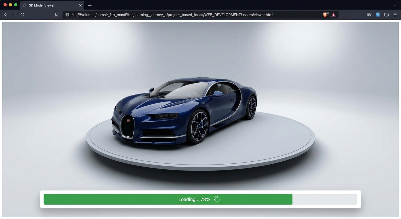
The Core Question You Are Answering
“How do you load, inspect, modify, and present an external 3D model in Three.js with production-quality lighting, shadows, and animation playback?”
This matters because most Three.js applications work with external 3D assets created in Blender, Maya, or 3D scanning. Understanding the GLTF loading pipeline – from download to GPU – and how to traverse and modify the imported scene graph is a required skill for professional Three.js development.
Concepts You Must Understand First
- GLTFLoader and the GLTF Structure
- What does a loaded GLTF object contain (
gltf.scene,gltf.animations,gltf.cameras,gltf.asset)? - Reference: Three.js docs - GLTFLoader
- What does a loaded GLTF object contain (
- Scene Traversal with traverse()
- How do you walk through every node in the imported scene graph to enable shadows, modify materials, or collect statistics?
- Reference: Three.js docs - Object3D.traverse()
- DRACOLoader and Geometry Compression
- What is Draco compression, how does it reduce file size, and what is the trade-off (decompression cost)?
- Reference: Three.js examples - Draco loader
- AnimationMixer and AnimationAction
- How does the Three.js animation system play back keyframe animations embedded in GLTF files?
- Reference: Discover Three.js - The Animation System (online)
- Environment Maps and Image-Based Lighting (IBL)
- How does an HDR environment map provide both ambient lighting and material reflections?
- Reference: Three.js docs - PMREMGenerator, RGBELoader
- Auto-Centering and Scaling
- How do you compute the bounding box of an arbitrarily-sized model and normalize it to fit the viewport?
- Book Reference: “Math for Programmers” by Paul Orland - Ch. 3 (bounding boxes, min/max operations)
Questions to Guide Your Design
- Auto-Fit Logic
- How do you compute the bounding box of the loaded model and use it to center and scale the model to a standard size?
- Should you modify the model’s scale, or the camera’s position and FOV?
- Loading Progress
- The
LoadingManagerprovidesonProgress(url, loaded, total). How do you calculate the percentage and update the DOM progress bar? - What happens if the total is unknown (some servers do not send Content-Length)?
- The
- Contact Shadow
- Should you use real shadow mapping (accurate but expensive) or a blurred circle texture below the model (cheap and convincing)?
- How do you position the shadow plane at the bottom of the model’s bounding box?
- Animation Selection UI
- How do you crossfade between animations when the user selects a new one from the dropdown?
- What is
action.crossFadeTo()and how does it produce smooth transitions?
- Turntable vs User Control
- How do you implement turntable auto-rotation that pauses when the user interacts with OrbitControls?
- Can you use
controls.autoRotate = truefrom OrbitControls, or do you need a custom implementation?
Thinking Exercise
Exercise: Trace the GLTF Loading Pipeline
Draw a timeline showing what happens when a user visits the page and a GLTF model loads:
Time 0ms:   Page loads. WebGLRenderer, Scene, Camera initialized.
            LoadingManager starts tracking.
            GLTFLoader.load('model.glb') called.

Time 0-3000ms: Browser fetches model.glb (e.g., 5MB file).
               LoadingManager.onProgress fires:
                 "model.glb - 1MB / 5MB (20%)"
                 "model.glb - 3MB / 5MB (60%)"
                 "model.glb - 5MB / 5MB (100%)"

Time 3000ms: File download complete.
             GLTFLoader parses JSON metadata.
             If Draco-compressed: DRACOLoader spawns Web Worker,
               Worker decompresses geometry buffers (~200ms).

Time 3200ms: Textures are decoded by browser image decoders.
             gltf object is ready.

Time 3200ms: onLoad callback fires with gltf object.
             scene.add(gltf.scene) -- model appears.
             traverse() enables shadows on all meshes.
             BoundingBox computed, model centered and scaled.
             AnimationMixer created, first clip plays.
             Progress bar fades out.

Time 3200ms+: Render loop shows the model rotating on turntable.
Questions to answer:
- At what point could you show a low-resolution preview while the full model loads?
- Why does DRACOLoader use a Web Worker? What would happen without it? (The main thread would freeze during decompression)
- If the GLTF file references external .bin and .jpg files (not embedded), how many HTTP requests are made?
The Interview Questions They Will Ask
-
“What is GLTF, and why is it preferred over FBX or OBJ for web 3D?”
-
“How does Draco compression work, and what are the trade-offs between file size reduction and client-side decompression time?”
-
“Describe how you would auto-center and auto-scale any arbitrary GLTF model to fit within the camera’s view.”
-
“How does Three.js’s AnimationMixer work? Walk me through playing, pausing, and crossfading between animations.”
-
“What is the difference between using an HDR environment map for scene lighting versus using explicit light objects (DirectionalLight, PointLight)?”
-
“A loaded GLTF model appears too dark in your scene. What are the possible causes and how would you debug it?”
Hints in Layers
Hint 1: Basic Loading
Import GLTFLoader from three/addons/loaders/GLTFLoader.js. Use loader.loadAsync('model.glb') for a promise-based approach. The result contains gltf.scene (a Group you add to your scene) and gltf.animations (an array of AnimationClip). For the model URL, use free models from Sketchfab (download as GLTF) or Three.js examples.
Hint 2: Auto-Centering
After adding gltf.scene to your scene, compute its bounding box: const box = new THREE.Box3().setFromObject(gltf.scene). Get the center: box.getCenter(center). Get the size: box.getSize(size). Offset the model by the negative center so it sits at the origin. Compute the max dimension and scale or move the camera so the model fills the viewport. Use Math.max(size.x, size.y, size.z) for the dominant axis.
Hint 3: Environment Lighting
Import RGBELoader from three/addons/loaders/RGBELoader.js. Load an HDR file: new RGBELoader().load('studio.hdr', (texture) => { texture.mapping = THREE.EquirectangularReflectionMapping; scene.environment = texture; }). Setting scene.environment applies the HDR as ambient lighting and reflection source for all PBR materials in the scene. Optionally set scene.background = texture to show the environment as the background.
Hint 4: Animation Playback
Create a mixer: mixer = new THREE.AnimationMixer(gltf.scene). For each animation clip: action = mixer.clipAction(clip); action.play(). In the render loop: mixer.update(delta). For crossfading: call currentAction.crossFadeTo(newAction, 0.5); newAction.play(). The 0.5 is the blend duration in seconds. Update the mixer’s time scale with mixer.timeScale = speedSlider.value for speed control.
Books That Will Help
| Topic | Book | Chapter |
|---|---|---|
| Scene description and rendering | “Computer Graphics from Scratch” by Gabriel Gambetta | Ch. 10 - Describing and Rendering a Scene |
| Shading and lighting models | “Computer Graphics from Scratch” by Gabriel Gambetta | Ch. 13 - Shading |
| Bounding box math | “Math for Programmers” by Paul Orland | Ch. 3 - Ascending to the 3D World |
| Matrix transforms for auto-centering | “Math for Programmers” by Paul Orland | Ch. 5 - Computing Transformations with Matrices |
| PBR and environment lighting (advanced) | “Real-Time Rendering” by Akenine-Moller et al. | Ch. 4 - Visual Appearance |
Common Pitfalls and Debugging
Problem 1: “Model loads but is invisible or extremely tiny”
- Why: The model’s scale is vastly different from your scene scale. Some models are in millimeters (a shoe is 300 units tall) while your camera expects objects around 1-10 units.
- Fix: Compute the bounding box, find the max dimension, and scale the model so the max dimension equals a target size (e.g., 5 units). Or move the camera to match the model’s scale.
- Quick test: Log
box.getSize(new THREE.Vector3())to see the model’s actual dimensions.
Problem 2: “DRACOLoader fails with ‘decoder not found’ error”
- Why: The Draco decoder WASM/JS files are not served from the correct path. DRACOLoader needs static decoder files.
- Fix: Set
dracoLoader.setDecoderPath('/draco/')and ensure the Draco decoder files (draco_decoder.js,draco_wasm_wrapper.js,draco_decoder.wasm) are in yourpublic/draco/directory. Copy them fromnode_modules/three/examples/jsm/libs/draco/. - Quick test: Check the browser Network tab for 404 errors on draco_decoder files.
Problem 3: “Model appears pitch black despite having a HDR environment”
- Why: The model’s materials are not PBR (some GLTF exporters produce unlit or Phong materials), or the environment map is not set correctly, or
scene.environmentwas set before the HDR loaded. - Fix: Traverse the model and log each material type. If materials are
MeshBasicMaterial, they will not respond to environment lighting. Convert them toMeshStandardMaterialif needed. Ensurescene.environment = textureis called after the HDR texture loads. - Quick test: Set
scene.background = scene.environment– if you see the HDR image as background but the model is still dark, the issue is with the model’s materials.
Problem 4: “Animations are not playing or play incorrectly”
- Why:
mixer.update(delta)is not being called in the render loop, ordeltais always 0, or the AnimationAction was never started with.play(). - Fix: Ensure
clock.getDelta()is called exactly once per frame and the result is passed tomixer.update(). Verifygltf.animations.length > 0. Callaction.play()after creating the action. - Quick test: Log
mixer.timeeach frame – it should increase steadily.
Definition of Done
- GLTF/GLB model loads and displays correctly in the viewer
- Loading progress bar shows percentage and disappears when loading completes
- Model is auto-centered and auto-scaled to fit the viewport
- Ground plane with contact shadow is visible beneath the model
- HDR environment provides PBR-quality lighting and reflections
- Model slowly rotates on a turntable (auto-rotation)
- OrbitControls allows manual camera control (pauses turntable)
- If the model has animations, the first animation plays on loop
- Animation controls (play/pause, speed) are functional
- Model info (triangles, materials, animations) is displayed
- Draco-compressed models load correctly (if DRACOLoader is configured)
- No console errors during loading or interaction
Project 6: Physics-Based Playground
- File: P06-physics-playground.md
- Main Programming Language: JavaScript
- Alternative Programming Languages: TypeScript, React Three Fiber + @react-three/rapier
- Coolness Level: 4 - “Show this at a party” (satisfying, interactive, fun to play with)
- Business Potential: 1 - Resume / Portfolio Only
- Difficulty: Advanced - Open Problem (physics integration, two-world sync, collision handling)
- Knowledge Area: Physics Simulation / Game Development Foundations
- Software or Tool: Three.js, cannon-es (physics engine), Vite, lil-gui
- Main Book: “Math for Programmers” by Paul Orland - Ch. 8-9 (Rates of Change, Simulating Moving Objects)
What you will build: An interactive physics playground where clicking anywhere spawns objects (boxes, spheres) that fall under gravity, bounce off a ground plane, collide with each other, stack, and tumble. A pre-built tower of boxes can be knocked over by launching a sphere at it. Physics properties (restitution, friction, mass) are tunable via UI sliders.
Why it teaches Three.js: Three.js is a rendering library – it has zero built-in physics. Understanding how to integrate a separate physics engine (cannon-es), maintain two parallel worlds (visual + physics), synchronize their states every frame, and handle the fixed-timestep pattern is foundational for any Three.js game or simulation. This separation of concerns (render vs simulate) is a key architectural concept that applies to audio engines, networking, and AI systems as well.
Core challenges you will face:
- Two-world synchronization -> Maps to keeping Three.js meshes and cannon-es rigid bodies in sync each frame
- Fixed timestep vs variable render rate -> Maps to physics stability and the accumulator pattern
- Contact materials and material pairs -> Maps to configuring friction and restitution between different object types
- Object spawning and lifecycle management -> Maps to creating and destroying both physics bodies and visual meshes
Real World Outcome
When you open the page in a browser:
Initial Scene: A large, flat ground plane stretches across the viewport (a muted gray or green surface). On the right side of the ground, a tower of 10-15 stacked boxes stands upright. Each box is a slightly different color (randomly generated pastel shades). The tower is 5 boxes tall and 3 wide, neatly stacked. The scene is lit by a directional light casting shadows, giving the tower a solid, physical presence.
Click to Spawn: Clicking anywhere in the 3D scene spawns a random object (box or sphere, chosen randomly) at a height of 10 units above the click point. The object has a random color and a mass of 1 unit. It immediately begins falling due to gravity (9.82 m/s^2 downward). The object:
- Falls with realistic acceleration (not constant velocity)
- Bounces on the ground plane with a restitution of 0.3 (moderate bounce, losing energy each bounce)
- Slides with friction (coefficient 0.5) – spheres roll, boxes slide and tip
- Stacks on top of other fallen objects if it lands squarely
- After 3-4 bounces, the object settles to rest
Tower Demolition: Clicking near the base of the tower launches a sphere projectile at high velocity toward the tower. The sphere impacts the tower, sending boxes flying, tumbling, and cascading. The boxes interact with each other: a falling box hits another, which hits another, creating a satisfying chain reaction. Some boxes fly off the ground plane. Others stack in new configurations. The physics simulation handles all of this automatically.
UI Controls (lil-gui): A debug panel allows tuning:
- Restitution (0.0 - 1.0): How bouncy objects are. At 1.0, objects bounce forever. At 0.0, they stop dead.
- Friction (0.0 - 2.0): How much objects resist sliding. High friction makes objects grip; low friction makes them slide like ice.
- Mass (0.1 - 10.0): How heavy spawned objects are. Heavier objects push lighter ones out of the way.
- Gravity (-20 to 0): Strength of gravity. Setting to 0 creates a zero-G environment.
- Reset button: Clears all spawned objects and rebuilds the tower.
Physics Feel: Objects feel “real.” Spheres roll and settle. Boxes tip over if pushed off-balance. Stacked objects compress the tower. A heavy sphere launched at the tower produces a dramatic collapse. Nothing clips through the floor. Nothing vibrates or jitters (the physics timestep is fixed).
Console Verification:
- Each spawned object creates exactly one draw call (one mesh + one physics body)
renderer.info.render.callsincreases by 1 per spawned object- Physics world body count matches visual scene object count
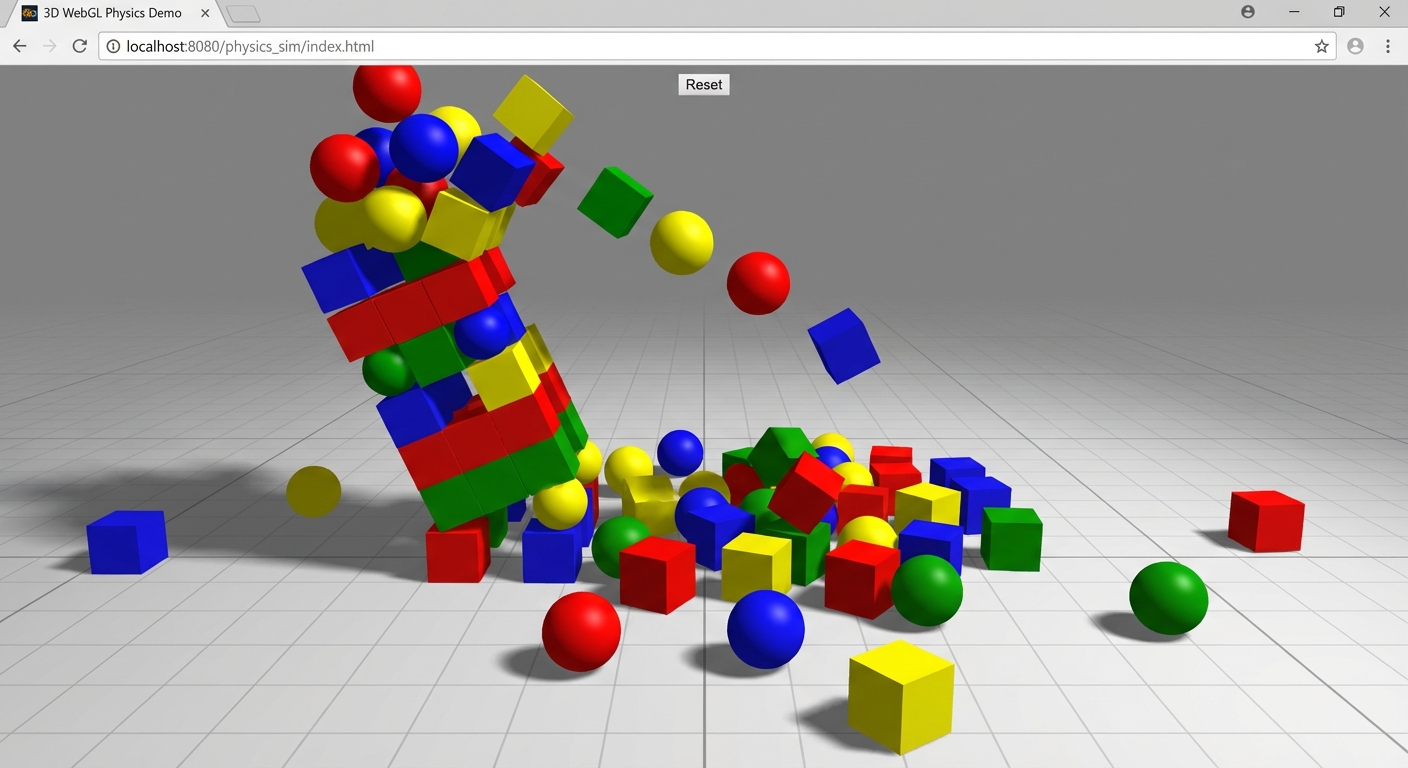
The Core Question You Are Answering
“How do you integrate a physics engine with Three.js, and what is the architectural pattern for keeping the visual world and the physics world synchronized?”
This matters because any Three.js application that simulates physical behavior – games, product demonstrations with gravity, data visualizations with collisions, interactive simulations – requires this exact two-world synchronization pattern. The physics engine computes positions and rotations; Three.js renders them. They run in lockstep but at potentially different rates.
Concepts You Must Understand First
- Rigid Body Physics
- What is a rigid body, and how does a physics engine compute its position each frame using forces, velocity, and acceleration?
- Book Reference: “Math for Programmers” by Paul Orland - Ch. 8 (Rates of Change) and Ch. 9 (Simulating Moving Objects)
- Two-World Architecture
- Why does the physics engine maintain a separate world from Three.js, and why can they not share the same objects?
- Reference: cannon-es documentation - Getting Started
- Fixed Timestep and the Accumulator Pattern
- Why must physics use a fixed timestep (e.g., 1/60s) instead of the variable frame delta, and how does the accumulator pattern work?
- Reference: “Fix Your Timestep!” by Glenn Fiedler (gaffer.games)
- Collision Detection (Broadphase and Narrowphase)
- What is the difference between broadphase (quick AABB rejection) and narrowphase (precise shape intersection), and why do physics engines use both?
- Reference: cannon-es docs - Broadphase
- Contact Materials
- How do friction and restitution values interact between two colliding objects, and what is a ContactMaterial in cannon-es?
- Reference: cannon-es docs - Materials and ContactMaterial
- Object Lifecycle Management
- How do you spawn and destroy objects in both the physics world and the visual scene without memory leaks?
- Reference: Three.js docs - dispose(), cannon-es World.removeBody()
Questions to Guide Your Design
- World Initialization
- How do you create the cannon-es
Worldwith gravity, and what broadphase algorithm should you use for a small-to-medium number of objects? - What are the differences between
NaiveBroadphaseandSAPBroadphase?
- How do you create the cannon-es
- Body-Mesh Pairing
- How will you track which physics body corresponds to which Three.js mesh? An array of pairs? A Map? A property on the mesh?
- What happens if you remove a mesh but forget to remove its physics body (or vice versa)?
- Spawn Mechanics
- When the user clicks, how do you convert the 2D click position into a 3D spawn position above the ground?
- Should objects spawn at the click point projected onto the ground, or at the camera position and launched toward the click point?
- Tower Construction
- How do you programmatically stack boxes in a tower formation with correct physics? Do you need to wait for physics to settle before adding the next layer?
- What spacing prevents the tower from immediately collapsing due to interpenetrating physics bodies?
- Performance and Cleanup
- What happens if the user spawns 500 objects? How do you limit the number of physics bodies for performance?
- Should you remove objects that fall off the ground plane or that have been resting for a long time?
Thinking Exercise
Exercise: Draw the Two-World Architecture
On paper, draw two parallel columns: “Physics World (cannon-es)” and “Visual World (Three.js).” For each spawned object, show:
Physics World (cannon-es)         Visual World (Three.js)
------------------------------    ----------------------------
World                             Scene
  gravity: (0, -9.82, 0)           |-- DirectionalLight
  |                                 |-- AmbientLight
  |-- Body (ground)                 |-- Mesh (ground plane)
  |     shape: Plane                |     geometry: PlaneGeometry
  |     mass: 0 (static)           |     material: MeshStandard
  |     position: (0, 0, 0)        |     position: (0, 0, 0)
  |                                 |
  |-- Body (box1)                   |-- Mesh (box1)
  |     shape: Box(0.5, 0.5, 0.5)  |     geometry: BoxGeometry(1,1,1)
  |     mass: 1                     |     material: MeshStandard
  |     position: updates...        |     position: copies from body
  |                                 |
  |-- Body (sphere1)                |-- Mesh (sphere1)
       shape: Sphere(0.5)               geometry: SphereGeometry(0.5)
       mass: 1                           material: MeshStandard
       position: updates...              position: copies from body

Sync Loop (every frame):
  1. world.step(1/60, delta, 3)    <-- physics updates body positions
  2. For each (body, mesh) pair:
       mesh.position.copy(body.position)
       mesh.quaternion.copy(body.quaternion)
  3. renderer.render(scene, camera) <-- visual world draws current state
Questions to answer:
- Why is the ground body’s mass 0? (Mass 0 = static body, infinite mass, never moves)
- Why do we copy
quaternioninstead ofrotation? (Cannon-es uses quaternions; copying directly avoids Euler angle conversion) - What happens if step 2 is skipped? (Meshes stay at their spawn position while invisible physics bodies move)
- Why does
world.step(1/60, delta, 3)have three arguments? (Fixed timestep, actual delta, max substeps for catch-up)
The Interview Questions They Will Ask
-
“Three.js does not have built-in physics. How do you integrate a physics engine like cannon-es or Rapier with Three.js?”
-
“Explain the fixed timestep pattern. Why can you not simply pass the frame delta directly to the physics step?”
-
“What is the difference between a static body, a dynamic body, and a kinematic body in a physics engine?”
-
“How do friction and restitution interact when two objects with different materials collide?”
-
“You have a scene with 1,000 dynamic physics objects and the frame rate drops to 15fps. What are three strategies to improve performance?”
-
“What is the ‘two-world problem’ in physics-rendered applications, and how do you keep the physics and visual representations in sync?”
Hints in Layers
Hint 1: Setting Up cannon-es
Install cannon-es: npm install cannon-es. Create a physics world: const world = new CANNON.World({ gravity: new CANNON.Vec3(0, -9.82, 0) }). Create a ground body: const groundBody = new CANNON.Body({ mass: 0, shape: new CANNON.Plane() }). Rotate the ground to be horizontal: groundBody.quaternion.setFromEuler(-Math.PI / 2, 0, 0). Add to world: world.addBody(groundBody).
Hint 2: Body-Mesh Pair Management
Maintain an array: const objectPairs = []. When spawning an object, create both the physics body and the visual mesh, then push { body, mesh } into the array. In the animation loop after world.step(), iterate over objectPairs and copy: pair.mesh.position.copy(pair.body.position); pair.mesh.quaternion.copy(pair.body.quaternion).
Hint 3: Spawn on Click
Use raycasting to find the click point on the ground plane: raycaster.setFromCamera(mouse, camera); const hits = raycaster.intersectObject(groundMesh); if (hits.length > 0) { const spawnPoint = hits[0].point; spawnPoint.y = 10; // spawn above }. Create a body at spawnPoint with a downward initial velocity of 0 (gravity does the rest). Create a matching mesh and add both to their respective worlds.
Hint 4: Contact Materials
Create materials: const defaultMaterial = new CANNON.Material('default'). Create a contact material: const contactMaterial = new CANNON.ContactMaterial(defaultMaterial, defaultMaterial, { friction: 0.5, restitution: 0.3 }). Add to world: world.addContactMaterial(contactMaterial). Set the default material on all bodies: body.material = defaultMaterial. Expose friction and restitution in lil-gui, updating the contactMaterial values when sliders change.
Books That Will Help
| Topic | Book | Chapter |
|---|---|---|
| Rates of change and velocity | “Math for Programmers” by Paul Orland | Ch. 8 - Rates of Change |
| Simulating moving objects | “Math for Programmers” by Paul Orland | Ch. 9 - Simulating Moving Objects |
| Force fields and physics | “Math for Programmers” by Paul Orland | Ch. 10 - Working with Symbolic Expressions |
| 3D coordinate systems | “Math for Programmers” by Paul Orland | Ch. 3 - Ascending to the 3D World |
| Vectors for force/velocity | “Math for Programmers” by Paul Orland | Ch. 2 - Drawing with 2D Vectors |
Common Pitfalls and Debugging
Problem 1: “Objects fall through the ground”
- Why: The ground plane’s physics body is not rotated to be horizontal (cannon-es Plane shape defaults to XZ, not horizontal), or the ground body was never added to the world, or the physics timestep is too large causing tunneling.
- Fix: Rotate the ground body quaternion:
groundBody.quaternion.setFromEuler(-Math.PI / 2, 0, 0). Verifyworld.bodies.includes(groundBody). Useworld.step(1/60, delta, 3)with max substeps to prevent tunneling at low frame rates. - Quick test: Spawn a sphere directly above the ground at (0, 5, 0). Does it stop at y = 0.5 (sphere radius)?
Problem 2: “Objects jitter or vibrate when resting”
- Why: The physics solver is fighting gravity every frame on resting objects. Without sleeping or damping, objects never fully settle.
- Fix: Enable sleeping:
world.allowSleep = true. Set sleep speed threshold:body.sleepSpeedLimit = 0.1; body.sleepTimeLimit = 1. Add linear and angular damping:body.linearDamping = 0.1; body.angularDamping = 0.1. This allows objects to “sleep” when their velocity drops below the threshold. - Quick test: Spawn a single box. After it bounces and settles, check
body.sleepState– it should beCANNON.Body.SLEEPING(value 2).
Problem 3: “Spawning many objects tanks the frame rate”
- Why: Each physics body adds to the broad-phase computation cost, and each mesh adds a draw call. Beyond 200-300 dynamic bodies, cannon-es struggles.
- Fix: Set a maximum object count (e.g., 100). When exceeded, remove the oldest objects:
world.removeBody(pair.body); scene.remove(pair.mesh); pair.mesh.geometry.dispose(); pair.mesh.material.dispose(); objectPairs.shift(). Consider usingSAPBroadphaseinstead ofNaiveBroadphasefor better performance. - Quick test: Monitor
renderer.info.render.callsand aim to keep it under 150.
Problem 4: “Tower collapses immediately on scene load”
- Why: Physics bodies are overlapping when created (boxes are exactly touching or interpenetrating). The physics solver pushes them apart violently.
- Fix: Add a tiny gap (0.01-0.05 units) between stacked boxes. Create the tower with boxes at positions like
y = 0.5, 1.55, 2.60instead ofy = 0.5, 1.5, 2.5. Allow the physics world to settle for a few frames before enabling user interaction. - Quick test: Start the simulation and watch the tower for 2 seconds. If it explodes, increase the spacing between boxes.
Definition of Done
- Ground plane is visible and acts as a solid surface for physics objects
- Clicking spawns a random object (box or sphere) that falls under gravity
- Objects bounce with configurable restitution (bounciness)
- Objects slide with configurable friction
- Objects collide with each other realistically (stacking, tumbling)
- A pre-built tower of boxes stands stable until disturbed
- Launching a projectile at the tower causes a satisfying collapse
- lil-gui controls allow real-time tuning of restitution, friction, mass, and gravity
- Reset button clears all spawned objects and rebuilds the tower
- Physics timestep is fixed (1/60s) regardless of frame rate
- No objects fall through the ground
- No jittering of resting objects (sleeping is enabled)
- Memory is managed (old objects are removed when count exceeds limit)
Project 7: Custom Shader Water
- File: P07-custom-shader-water.md
- Main Programming Language: JavaScript + GLSL
- Alternative Programming Languages: TypeScript + GLSL, JavaScript + TSL (Three Shading Language)
- Coolness Level: 5 - “I need to show everyone” (mesmerizing, art-gallery quality)
- Business Potential: 1 - Resume / Portfolio Only
- Difficulty: Expert - Research Required (shader programming, GLSL, noise functions, GPU thinking)
- Knowledge Area: Shaders / GPU Programming / Procedural Generation
- Software or Tool: Three.js, ShaderMaterial, GLSL, Vite, lil-gui
- Main Book: “The Book of Shaders” by Patricio Gonzalez Vivo (online, free) + “Computer Graphics from Scratch” by Gabriel Gambetta - Ch. 13 (Shading)
What you will build: A mesmerizing procedural water surface where waves are generated entirely by GPU noise functions in a custom vertex and fragment shader. The water surface undulates with layered noise, colors shift from deep blue in troughs to white foam on wave peaks, and the animation runs endlessly at 60fps because all computation happens on the GPU.
Why it teaches Three.js: Custom shaders are the key that unlocks everything Three.js’s built-in materials cannot do. Understanding vertex and fragment shaders, uniforms, varyings, and GLSL is what separates a Three.js user from a Three.js developer. This project forces you to think in GPU terms: massively parallel computation, no conditionals, no state between pixels. You write code that runs simultaneously on thousands of GPU cores, producing a visual effect that would be impossible to achieve at interactive frame rates on the CPU.
Core challenges you will face:
- Writing GLSL vertex and fragment shaders from scratch -> Maps to GPU programming paradigm (parallel, stateless)
- Implementing noise functions for organic motion -> Maps to Simplex/Perlin noise theory and FBM layering
- Passing data between JavaScript and GLSL via uniforms -> Maps to CPU-GPU communication pattern
- Using varyings to pass data from vertex to fragment shader -> Maps to interpolated per-vertex data across triangles
- Thinking in terms of per-vertex and per-pixel operations -> Maps to GPU execution model
Real World Outcome
When you open the page in a browser:
Initial Impression: A large, undulating water surface fills the viewport. The surface is a subdivision-heavy plane (e.g., 256x256 segments) that appears to have real 3D waves. This is not a flat plane with a wave texture – the vertices themselves move up and down, creating genuine 3D displacement visible from any angle.
Wave Animation: Multiple layers of waves at different frequencies and amplitudes combine to create organic, ocean-like motion:
- Large swells: Slow, wide waves with amplitudes of 0.5-1.0 units, traveling across the surface at a steady pace. These form the “base layer” of the ocean.
- Medium waves: Faster, narrower waves layered on top of the swells, adding detail and complexity. These have roughly half the amplitude and twice the frequency of the large waves.
- Small ripples: High-frequency, low-amplitude perturbations that add surface texture and catch the light. These are the “frosting” that makes the water look realistic.
The waves are generated by Fractal Brownian Motion (FBM) – multiple octaves of simplex or Perlin noise layered together, each octave at double the frequency and half the amplitude of the previous one. The noise function receives position.xz + time * direction as input, producing a smooth, continuous, never-repeating wave pattern.
Color Variation: The water color varies based on wave height:
- Deep troughs: Dark blue (#003366 or similar) – the low points of the waves appear as deep water
- Mid-height: Ocean blue (#006699) – the main body of the water surface
- Near peaks: Lighter blue-green (#33cccc) – the crests lighten as they catch light
- Peak foam: White or near-white (#ccffff to #ffffff) – the very tips of the highest waves appear as foam
This color mapping is done in the fragment shader using the height value passed as a varying from the vertex shader. A mix() or smoothstep() function blends between the deep blue and foam white based on normalized height.
Lighting and Specular: A directional “sun” light illuminates the water from an angle. The fragment shader computes basic diffuse and specular lighting:
- The surface normal is recomputed in the vertex shader after displacement (by sampling the noise at slightly offset positions and computing the cross product)
- Specular highlights dance across the wave crests as the surface moves, creating glittering “sun sparkles”
- The specular contribution is brightest at the peaks where normals are most aligned with the light reflection
Performance: The animation runs at a locked 60fps on any modern GPU because:
- All displacement computation happens in the vertex shader (per-vertex, parallel)
- All color computation happens in the fragment shader (per-pixel, parallel)
- JavaScript only updates one uniform (
uTime) each frame – no CPU-side geometry updates - The noise functions are pure math with no texture lookups
lil-gui Controls:
- Wave Height (0.0 - 3.0): Controls the maximum displacement amplitude
- Wave Speed (0.0 - 5.0): Controls how fast waves travel across the surface
- Noise Octaves (1 - 6): Controls how many FBM layers are used (more = more detailed but slower)
- Foam Threshold (0.0 - 1.0): Controls at what height foam appears
- Deep Color: Color picker for the trough color
- Foam Color: Color picker for the peak color
- Sun Direction: Controls the light direction for specular highlights
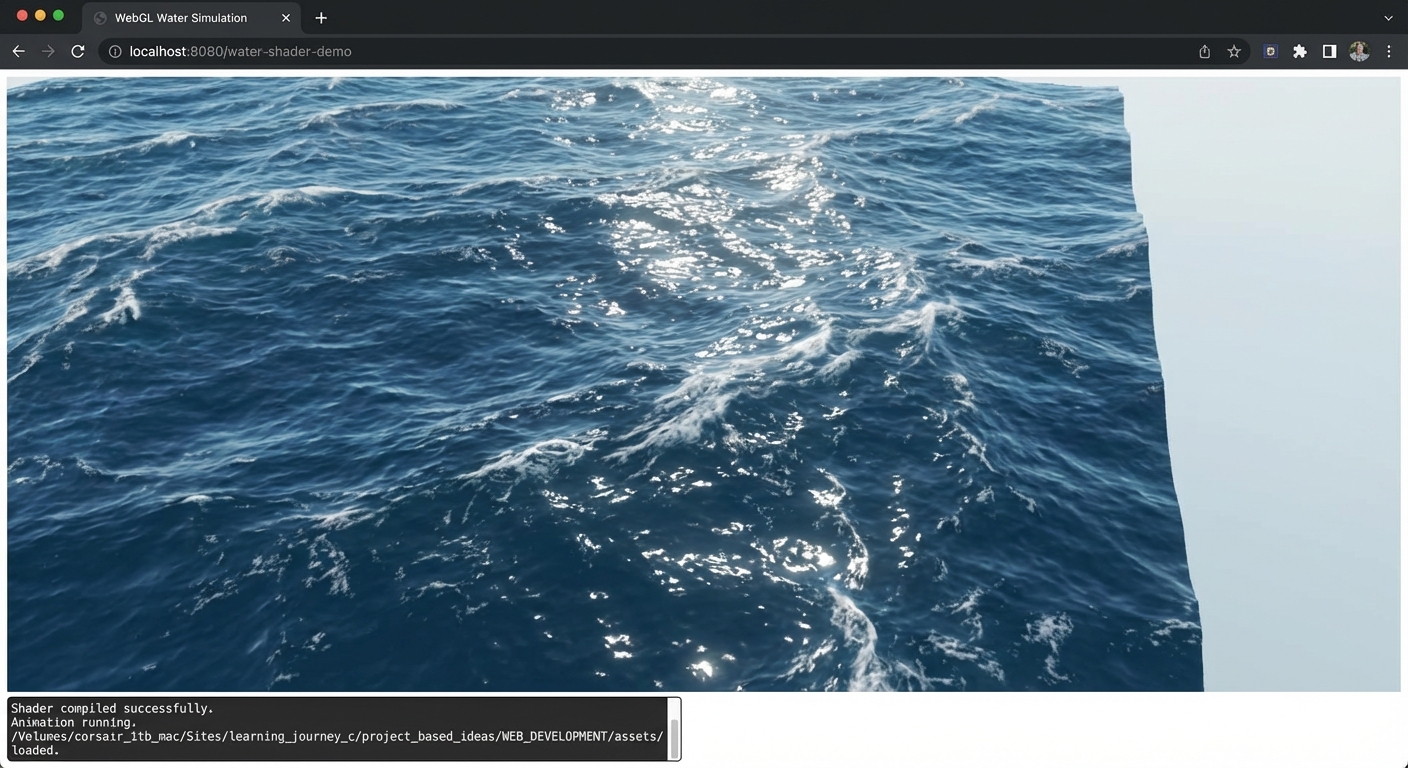
The Core Question You Are Answering
“How do you write custom GPU programs (shaders) in Three.js to create visual effects that are impossible with built-in materials, and how do you think in the massively parallel GPU paradigm?”
This matters because shaders are what make the best Three.js work stand out. Every award-winning Three.js site uses custom shaders. The jump from “I use MeshStandardMaterial” to “I write my own shaders” is the jump from consumer to creator.
Concepts You Must Understand First
- Vertex Shader Fundamentals
- What data does a vertex shader receive (attributes), what does it output (gl_Position, varyings), and when does it run?
- Book Reference: “Computer Graphics from Scratch” by Gabriel Gambetta - Ch. 13 (Shading) and Ch. 6 (Filled Triangles)
- Fragment Shader Fundamentals
- What data does a fragment shader receive (varyings, uniforms), what does it output (gl_FragColor), and how is it different from a vertex shader?
- Reference: “The Book of Shaders” by Patricio Gonzalez Vivo - Chapters 1-5
- Uniforms, Attributes, and Varyings
- How do uniforms pass data from JavaScript to GLSL? How do attributes provide per-vertex data? How do varyings pass interpolated data from vertex to fragment shader?
- Reference: Three.js docs - ShaderMaterial, uniforms
- Noise Functions (Simplex/Perlin/FBM)
- What makes noise functions smooth and continuous, and how does Fractal Brownian Motion layer multiple octaves for natural-looking results?
- Reference: “The Book of Shaders” - Chapter on Noise (https://thebookofshaders.com/11/)
- GLSL Data Types and Operations
- What are
vec2,vec3,vec4,mat4? How domix(),smoothstep(),clamp(), and swizzle notation work? - Reference: “The Book of Shaders” - Chapter on Shaping Functions (https://thebookofshaders.com/05/)
- What are
- Normal Recomputation After Displacement
- When you displace vertices, the original normals are wrong. How do you compute new normals from the displaced surface?
- Book Reference: “Computer Graphics from Scratch” by Gabriel Gambetta - Ch. 8 (Shaded Triangles, normal computation)
Questions to Guide Your Design
- Geometry Resolution
- How many segments does your PlaneGeometry need for the displacement to look smooth? What is the visual difference between 64x64 and 256x256 segments?
- At what segment count does performance start to degrade?
- Noise Function Choice
- Will you use Simplex noise, Perlin noise, or Worley noise? Can you find a GLSL noise implementation that works in WebGL (no texture-based noise)?
- The popular
webgl-noiselibrary by Ashima Arts provides Simplex noise in pure GLSL – should you include it inline or as a separate file?
- FBM Parameters
- How many octaves of noise should you layer? What ratio of frequency doubling (lacunarity) and amplitude halving (gain) produces the most natural result?
- Should these be hardcoded or exposed as uniforms for real-time tuning?
- Color Mapping Strategy
- Should you pass the wave height from vertex to fragment shader as a varying, then use
mix()to blend colors based on height? - How do you define the color stops (deep blue at bottom, foam at top) in GLSL?
- Should you pass the wave height from vertex to fragment shader as a varying, then use
- Specular Highlight Computation
- How do you compute specular highlights in the fragment shader without relying on Three.js’s built-in lighting?
- Will you use the Phong specular model (reflect vector dot view vector) or Blinn-Phong (half vector dot normal)?
- Normal Computation
- After displacing vertices with noise, how do you compute the correct normal at each vertex?
- The finite-difference method: sample noise at
(x + epsilon, z)and(x, z + epsilon), compute the partial derivatives, then cross product. How small should epsilon be?
Thinking Exercise
Exercise: Think in Parallel
Imagine a PlaneGeometry with 256x256 segments = 66,049 vertices. When the vertex shader runs, all 66,049 executions happen simultaneously on the GPU. Each execution:
- Receives its own
positionattribute (unique x, y, z for this vertex) - Receives the same
uTimeuniform (current time, same for all vertices) - Computes
height = fbm(position.xz + uTime * waveDirection)using Simplex noise - Sets
position.y = height * amplitude - Computes a new normal by sampling noise at nearby points
- Passes
vHeight(the height value) andvNormal(the new normal) as varyings to the fragment shader - Transforms the displaced position to clip space:
gl_Position = projectionMatrix * modelViewMatrix * vec4(displacedPosition, 1.0)
Then the fragment shader runs once per pixel (millions of executions in parallel):
- Receives interpolated
vHeightandvNormalfrom the rasterizer - Maps
vHeightto a color:mix(deepBlue, foamWhite, smoothstep(0.3, 0.8, vHeight)) - Computes diffuse lighting:
max(dot(vNormal, lightDirection), 0.0) * lightColor - Computes specular:
pow(max(dot(reflect(-lightDir, vNormal), viewDir), 0.0), shininess) - Outputs
gl_FragColor = vec4(baseColor * diffuse + specular, 1.0)
Questions to answer:
- Why can vertex 12,345 not read the position of vertex 12,346? (GPU executions are independent – no shared state between shader invocations)
- If you change
uTimefrom JavaScript every frame, does the GPU need to re-upload all vertex data? (No – only the uniform value changes, which is tiny) - Why does a 256x256 plane with a noise shader run faster than updating 66,049 vertex positions in JavaScript? (GPU has thousands of cores running in parallel vs CPU single-thread)
- What happens if you use
if (height > 0.5) { color = white; } else { color = blue; }instead ofmix()in the fragment shader? (Hard edge instead of smooth gradient – branching is also slower on GPUs)
The Interview Questions They Will Ask
-
“What is the difference between a vertex shader and a fragment shader? When does each run?”
-
“Explain uniforms, attributes, and varyings. How does data flow from JavaScript to the vertex shader to the fragment shader?”
-
“What is Fractal Brownian Motion (FBM), and why is it used for procedural textures and terrain?”
-
“How would you compute surface normals after displacing vertices in a vertex shader?”
-
“Why are shaders inherently parallel? What restrictions does this parallel execution impose on shader code?”
-
“What is the difference between
ShaderMaterialandRawShaderMaterialin Three.js? When would you use each?”
Hints in Layers
Hint 1: ShaderMaterial Setup
Create a ShaderMaterial with vertexShader and fragmentShader strings, plus a uniforms object: { uTime: { value: 0.0 }, uAmplitude: { value: 1.0 }, uSpeed: { value: 1.0 }, uDeepColor: { value: new THREE.Color(0x003366) }, uFoamColor: { value: new THREE.Color(0xccffff) } }. In the render loop, update material.uniforms.uTime.value = clock.getElapsedTime(). Apply this material to a PlaneGeometry(20, 20, 256, 256) rotated to face upward.
Hint 2: Including Noise in GLSL
Copy a Simplex noise function (e.g., from the Ashima Arts webgl-noise repository, snoise(vec3) function) into the top of your vertex shader string. Then write an FBM function that layers multiple octaves:
// Pseudocode -- not runnable, but shows the pattern
float fbm(vec3 p) {
    float value = 0.0;
    float amplitude = 0.5;
    float frequency = 1.0;
    for (int i = 0; i < OCTAVES; i++) {
        value += amplitude * snoise(p * frequency);
        frequency *= 2.0;   // lacunarity
        amplitude *= 0.5;   // gain
    }
    return value;
}
Use this in the vertex shader: float h = fbm(vec3(position.x + uTime * uSpeed, 0.0, position.z + uTime * uSpeed * 0.7)); position.y = h * uAmplitude;
Hint 3: Height-Based Coloring in Fragment Shader
Pass the height from vertex to fragment shader: varying float vHeight; in both shaders, set vHeight = h; in vertex shader. In the fragment shader, compute the base color: vec3 color = mix(uDeepColor, uFoamColor, smoothstep(0.0, 1.0, (vHeight / uAmplitude + 1.0) * 0.5));. The smoothstep normalizes the height range and creates a smooth blend. Add a white foam overlay at peaks: color += vec3(smoothstep(0.7, 1.0, vHeight / uAmplitude) * 0.5);.
Hint 4: Normal Recomputation In the vertex shader, after computing the displaced height at the current vertex, sample the noise at two nearby points:
// Pseudocode
float eps = 0.1;
float hR = fbm(vec3(position.x + eps + uTime * uSpeed, 0.0, position.z));
float hF = fbm(vec3(position.x + uTime * uSpeed, 0.0, position.z + eps));

vec3 tangent = normalize(vec3(eps, (hR - h) * uAmplitude, 0.0));
vec3 bitangent = normalize(vec3(0.0, (hF - h) * uAmplitude, eps));
vec3 newNormal = normalize(cross(bitangent, tangent));
Pass newNormal to the fragment shader as a varying for lighting calculations. This finite-difference approach gives you approximate but visually convincing normals for any noise-displaced surface.
Books That Will Help
| Topic | Book | Chapter |
|---|---|---|
| Fragment shader fundamentals | “The Book of Shaders” by Patricio Gonzalez Vivo | Ch. 1-5 (online, free) |
| Noise functions and FBM | “The Book of Shaders” by Patricio Gonzalez Vivo | Ch. 11 - Noise (online, free) |
| Shading and illumination models | “Computer Graphics from Scratch” by Gabriel Gambetta | Ch. 13 - Shading |
| Texture mapping and UV coordinates | “Computer Graphics from Scratch” by Gabriel Gambetta | Ch. 14 - Textures |
| Vectors and cross products for normals | “Math for Programmers” by Paul Orland | Ch. 3 - Ascending to the 3D World |
| Transformations and matrices | “Math for Programmers” by Paul Orland | Ch. 5 - Computing Transformations with Matrices |
Common Pitfalls and Debugging
Problem 1: “Shader compilation error: random/noise function not found”
- Why: GLSL does not have a built-in Simplex or Perlin noise function. You must include the noise function source code in your shader string.
- Fix: Copy the complete
snoise(vec3)function from a trusted GLSL noise library (Ashima Arts webgl-noise) and paste it at the top of your vertex shader string, beforemain(). Ensure there are no syntax differences between GLSL versions. - Quick test: Replace the noise call with
sin(position.x + uTime)– if the shader compiles and produces sine waves, the noise function was the issue.
Problem 2: “Water surface is flat – no visible displacement”
- Why: The PlaneGeometry does not have enough segments (a 1x1 segment plane has only 4 vertices, so displacement has no visible effect), or the amplitude uniform is 0, or the displacement is applied in the wrong axis.
- Fix: Use at least 128x128 segments:
new PlaneGeometry(20, 20, 128, 128). VerifyuAmplitudeis greater than 0. Ensure displacement is applied to the Y component of position (after rotating the plane to be horizontal). - Quick test: Set amplitude very high (10.0) temporarily. If you still see no displacement, the issue is in the shader code, not the amplitude.
Problem 3: “Colors are uniform – no variation between troughs and peaks”
- Why: The
vHeightvarying is not being set in the vertex shader, or thesmoothsteprange does not match the actual height range, or the two colors are too similar. - Fix: Log the height range by temporarily using extreme colors (red for negative, green for positive). Adjust the
smoothstepparameters to match the actual minimum and maximum heights produced by your noise function. - Quick test: Set
gl_FragColor = vec4(vHeight, 0.0, 0.0, 1.0)in the fragment shader. The water should show red intensity varying with wave height.
Problem 4: “Specular highlights are missing or look like solid white patches”
- Why: Normals are not being recomputed after displacement (the original flat-plane normals all point straight up), or the specular power (shininess) is too low, or the view/light direction vectors are not being computed correctly.
- Fix: Implement the finite-difference normal recomputation in the vertex shader (see Hint 4). Pass the new normal as a varying. In the fragment shader, use the passed normal for the specular calculation. Set shininess to at least 64 for sharp highlights.
- Quick test: Temporarily set
gl_FragColor = vec4(vNormal * 0.5 + 0.5, 1.0)to visualize the normals. You should see a colorful surface where colors change with the wave slope.
Definition of Done
- Water surface displays visible 3D wave displacement (vertices actually move)
- Waves are generated by noise functions (FBM), not simple sine waves
- Multiple noise octaves create organic, ocean-like wave patterns
- Waves animate smoothly and endlessly using
uTimeuniform - Color varies from deep blue in troughs to white/foam on peaks
- Color transition is smooth (uses
mix()orsmoothstep()) - Specular highlights dance across wave crests
- Normals are recomputed after vertex displacement
- Performance stays at 60fps (all computation is on the GPU)
- lil-gui controls allow tuning wave height, speed, octaves, and colors
- No shader compilation errors in the console
- The effect is mesmerizing enough that you want to stare at it for more than 10 seconds
Project 8: Post-Processing Effects Gallery
- File: P08-post-processing-gallery.md
- Main Programming Language: JavaScript
- Alternative Programming Languages: TypeScript, Dart (Flutter WebGL)
- Coolness Level: 4 - Impressive (People lean in when they see it)
- Business Potential: 2 - Niche (Useful in specific domains)
- Difficulty: Intermediate
- Knowledge Area: Post-Processing / Compositing
- Software or Tool: Three.js, EffectComposer, lil-gui, stats.js
- Main Book: “Computer Graphics from Scratch” by Gabriel Gambetta - Ch. 13-14 (Shading, Textures)
What you will build: A gallery of post-processing effects applied to a 3D scene. The user clicks buttons to toggle effects on and off: Bloom, Film Grain, Vignette, Glitch, Pixelation, Color Grading, and Depth of Field. Multiple effects can stack simultaneously, and an FPS counter shows the performance impact of each effect.
Why it teaches Three.js: Post-processing is how professional 3D applications achieve cinematic quality. Understanding EffectComposer, render targets, ping-pong buffers, and full-screen shader passes bridges the gap between raw 3D rendering and polished visual output. This project forces you to understand the rendering pipeline beyond the initial scene render.
Core challenges you will face:
- Render Target Management -> Maps to concept: Post-Processing / Render Targets
- Effect Stacking and Pass Ordering -> Maps to concept: EffectComposer Pipeline
- Performance Measurement Under Load -> Maps to concept: Performance Optimization
- Custom Shader Passes -> Maps to concept: Shaders and GLSL
- Anti-Aliasing with Post-Processing -> Maps to concept: Rendering Pipeline
Real World Outcome
When you open the browser, you see a rotating torus knot geometry centered in the viewport against a dark background. The torus knot has a MeshStandardMaterial with moderate metalness and roughness, lit by a DirectionalLight from above-left and a subtle HemisphereLight for ambient fill. The knot rotates slowly on both X and Y axes. In the top-right corner, a stats.js panel shows FPS, MS per frame, and optionally GPU memory usage.
On the left side of the screen, a vertical panel of labeled toggle buttons is displayed using HTML/CSS overlay (not rendered in 3D). Each button has a name and an on/off state indicator. The buttons are:
-
Bloom - When toggled on, bright areas of the torus knot emit a soft glow that bleeds outward. The metallic highlights on the surface become luminous halos. The bloom spreads according to the UnrealBloomPass parameters: strength controls intensity (default 1.5), radius controls spread (default 0.4), and threshold controls which brightness values bloom (default 0.85). The dark background stays dark while only the bright specular highlights glow.
-
Film Grain - When toggled on, a subtle noise pattern overlays the entire image, flickering slightly each frame like analog film stock. The grain intensity is mild enough to add character without obscuring the 3D content. The noise pattern changes every frame, creating an organic cinematic feel.
-
Vignette - When toggled on, the edges and corners of the viewport gradually darken, drawing the viewer’s eye toward the center where the torus knot sits. The falloff is smooth and circular, strongest in the extreme corners.
-
Glitch - When toggled on, periodic digital distortion artifacts appear: horizontal scan lines shift, color channels separate momentarily, and blocks of pixels displace randomly. The effect triggers intermittently (not constantly), simulating digital signal corruption.
-
Pixelation - When toggled on, the rendered image is downsampled to a lower resolution and then upscaled, creating a retro blocky pixel art appearance. The torus knot becomes a mosaic of large colored squares. The pixel size is adjustable.
-
Color Grading - When toggled on, the overall color palette shifts. A lookup table or manual RGB curves apply a cinematic color tone – for example, shadows pushed toward teal and highlights pushed toward orange (the classic cinema look). The scene takes on a stylized, graded appearance.
-
Depth of Field - When toggled on, objects at a specific focal distance remain sharp while everything closer or farther blurs progressively. Since the scene has a single object, the focal point should be set on the torus knot, and the near/far regions blur subtly. If you move the camera closer or farther (via OrbitControls), the blur changes.
Clicking multiple buttons stacks effects: Bloom + Film Grain + Vignette together creates a cinematic look. Bloom + Glitch creates a cyberpunk aesthetic. Each time you toggle an effect, watch the FPS counter to see the performance cost. On a mid-range laptop, enabling all seven effects simultaneously might drop from 60fps to 30-40fps.
A lil-gui panel on the right side exposes the parameters for whichever effects are currently active: bloom strength/radius/threshold, grain intensity, vignette darkness/offset, glitch frequency, pixel size, DOF focus distance/aperture. Adjusting these sliders updates the visual output in real-time.
The total draw call count and triangle count (from renderer.info) are displayed below the FPS counter, letting you compare the rendering cost with zero effects versus all seven stacked.

The Core Question You Are Answering
“How does Three.js transform a finished 3D render into a cinematic image through chained full-screen shader passes, and what is the real performance cost of each effect?”
This question matters because post-processing is what separates amateur 3D demos from professional-quality output. Every AAA game, every film VFX pipeline, and every polished web experience uses post-processing. Understanding the EffectComposer pipeline – render targets, ping-pong buffers, full-screen quads, and shader passes – gives you the vocabulary and mental model to create any visual effect you can imagine. This project also teaches you to measure and reason about the GPU cost of visual quality, a skill critical for shipping real products.
The rendering pipeline does not end when renderer.render(scene, camera) completes. In production, that raw render is just the starting material. Post-processing transforms it through a chain of image-space operations – the same workflow used in film (color grading, lens effects) and games (bloom, motion blur, ambient occlusion). By building this gallery, you will understand exactly how each effect works at the shader level, and more importantly, you will develop the intuition for when each effect costs too much for your target platform.
Concepts You Must Understand First
- Render Targets and Framebuffer Objects (FBOs)
- What is a render target and why can’t you read and write the same one simultaneously?
- How does
WebGLRenderTargetdiffer from rendering directly to the screen canvas? - What dimensions should a render target have, and what happens when the window resizes?
- Book Reference: “Computer Graphics from Scratch” by Gabriel Gambetta - Ch. 14 (Textures, framebuffer concepts)
- The EffectComposer Pipeline
- How does EffectComposer chain passes, and what does ping-pong buffering mean?
- Why must the RenderPass always be the first pass in the chain?
- How does the
renderToScreenproperty on the final pass work? - Reference: Three.js docs - EffectComposer, Discover Three.js - Post-Processing chapter
- Full-Screen Quad Rendering
- Why does each post-processing pass render a full-screen quad, and how does this relate to fragment shaders?
- How does the UV coordinate system of the full-screen quad map to the previous pass’s output texture?
- Reference: “The Book of Shaders” - Fragment shader fundamentals
- Fragment Shader Basics
- How do you read from a texture in a fragment shader using
texture2D()and UV coordinates? - What is the
tDiffuseuniform and why does EffectComposer use that name by convention? - How do you manipulate per-pixel color values (brightness, contrast, hue) in a fragment shader?
- Book Reference: “Computer Graphics from Scratch” by Gabriel Gambetta - Ch. 13 (Shading)
- How do you read from a texture in a fragment shader using
- Performance Profiling with stats.js and renderer.info
- How do you measure FPS, draw calls, and triangle count in real-time?
- What does each metric tell you about where the bottleneck is (CPU vs GPU, vertex vs fragment)?
- How do you compare performance before and after adding an effect?
- Reference: Three.js docs - WebGLRenderer.info
Questions to Guide Your Design
- Pass Ordering
- Does the order of passes matter? What happens if you apply Bloom after Pixelation versus before? (Bloom after Pixelation would bloom the hard pixel edges, creating a soft glow around each block. Bloom before Pixelation would create smooth bloom that then gets pixelated, producing a different aesthetic.)
- Should anti-aliasing (FXAA) go first or last in the chain? (Always last – FXAA smooths aliased edges in the final image. Applying it before other effects would smooth edges that later effects might re-introduce.)
- Render Target Resolution
- Should every pass run at full viewport resolution, or can some effects run at half resolution for performance?
- How do you handle window resizing when render targets have fixed dimensions?
- What is the relationship between render target resolution and visual quality for each effect type?
- Toggle Architecture
- How do you dynamically add and remove passes from the EffectComposer without rebuilding the entire chain?
- What data structure tracks which effects are active?
- Do you maintain a fixed ordering of all possible effects and filter by active state, or insert/remove dynamically?
- Custom vs Built-In Passes
- Which effects have built-in Three.js passes (UnrealBloomPass, GlitchPass, FilmPass) and which require custom ShaderPass implementations (Vignette, Pixelation, Color Grading)?
- How do you write a custom ShaderPass? What is the minimum shader structure required?
- The custom shader must declare
uniform sampler2D tDiffuseto receive the previous pass’s output. The vertex shader passes through UVs. The fragment shader reads fromtDiffuseat each UV coordinate and applies the effect.
- Anti-Aliasing Considerations
- Why does the renderer’s built-in MSAA not work with post-processing? (MSAA operates on the main framebuffer. When rendering to a render target for post-processing, MSAA is bypassed because render targets do not support multisampling in WebGL 1.0.)
- How do you add FXAA or SMAA as a final pass?
- Parameter Exposure
- How do you connect lil-gui sliders to uniform values inside shader passes?
- How do uniforms update each frame without recreating the pass? (Uniforms are references – changing the
.valueproperty of a uniform object in JavaScript automatically updates the value for the next render. No pass recreation needed.) - Should you group parameters by effect in lil-gui folders for better organization?
Thinking Exercise
Exercise: Trace Data Flow Through a Three-Pass Chain
Diagram the data flow when Bloom, Vignette, and FXAA are all active:
3D Scene (meshes, lights, camera)
           |
           v
   +-------------------+
   |   RenderPass       |  Renders scene to Render Target A
   |   (scene, camera)  |  Output: Full 3D render as 2D texture
   +-------------------+
           |
           v
   +-------------------+
   |  UnrealBloomPass   |  Reads from Target A
   |                    |  Internal pipeline:
   |  1. Threshold pass |    Extract bright pixels
   |  2. Downscale 1/2  |    Reduce resolution
   |  3. Blur H pass    |    Horizontal Gaussian blur
   |  4. Blur V pass    |    Vertical Gaussian blur
   |  5. Downscale 1/4  |    Reduce further
   |  6. Blur H + V     |    Blur at lower resolution
   |  7. Upscale + blend|    Composite bloom onto original
   |                    |  Output: Bloomed image to Target B
   +-------------------+
           |
           v
   +-------------------+
   |  Vignette (custom) |  Reads from Target B
   |  ShaderPass        |  Multiplies each pixel by radial mask
   |                    |  Output: Vignetted image to Target A
   +-------------------+
           |
           v
   +-------------------+
   |  FXAA ShaderPass   |  Reads from Target A
   |  renderToScreen    |  Detects and smooths aliased edges
   |  = true            |  Output: Final image to SCREEN
   +-------------------+
Questions to answer:
- How many total render passes occur in this chain? (Count the internal bloom sub-passes too.) Hint: The RenderPass is 1. UnrealBloomPass internally runs approximately 7-9 sub-passes (threshold, multiple downsample/blur passes, upsample, composite). Vignette is 1. FXAA is 1. Total: roughly 10-12 full-screen renders per frame.
- If the viewport is 1920x1080, how many pixels does the fragment shader process per frame across all passes? (1920*1080 = ~2M pixels per full-resolution pass. Bloom’s downscaled passes process fewer pixels. Rough total: 10-15 million fragment shader invocations per frame.)
- What happens if you accidentally set
renderToScreen = trueon the Vignette pass instead of FXAA? (The vignetted image renders to screen, but FXAA also tries to render to screen – the final image may lack FXAA, or you see only the FXAA pass without the vignette, depending on the order.) - Why does Bloom internally use multiple render targets at different resolutions? (Blurring at lower resolution is exponentially cheaper. A Gaussian blur at 1/4 resolution covers the same spread as 4x the blur radius at full resolution, with 1/16th the pixel count. This is the “progressive downsampling” technique.)
The Interview Questions They Will Ask
- “Explain how the EffectComposer in Three.js works. What are render passes, and why does it use ping-pong buffers?”
- “Why can’t you use the renderer’s built-in multi-sample anti-aliasing (MSAA) when post-processing is active? What alternatives exist?”
- “If your post-processing chain is causing frame drops, what strategies would you use to optimize it without removing effects?”
- “How would you implement a custom post-processing effect that is not provided by Three.js, such as a CRT scanline effect?”
- “What is the difference between UnrealBloomPass and simply making emissive materials brighter? When would you choose one over the other?”
- “How does the bloom threshold parameter affect which pixels glow, and what problems arise if the threshold is set too low?”
Hints in Layers
Hint 1: Getting Started
Start by setting up a basic scene with a torus knot, one directional light, and OrbitControls. Verify the scene renders correctly with renderer.render(scene, camera) before adding any post-processing. Then replace the renderer call with an EffectComposer containing only a RenderPass. The visual output should be identical.
Hint 2: Adding Your First Effect
Import UnrealBloomPass from Three.js examples. Add it after the RenderPass. Experiment with the three parameters: strength (0 to 3), radius (0 to 1), and threshold (0 to 1). Observe how threshold controls which brightness values are affected. Lower threshold means more of the image blooms. Add a lil-gui panel to adjust these values live.
Hint 3: Building the Toggle System Create an object that maps effect names to their pass instances and a boolean for their active state. When a button is clicked, either add the pass to the composer (enable) or remove it (disable). Be careful: you must rebuild the pass chain in the correct order each time a toggle changes. Consider maintaining a fixed ordering array and filtering it by active state.
Hint 4: Custom Shader Passes
For effects like Vignette and Pixelation that lack built-in passes, create a custom shader object with uniforms, vertexShader, and fragmentShader properties. Wrap it in a ShaderPass. The vertex shader passes UVs through unchanged. The fragment shader reads the previous pass’s output via uniform sampler2D tDiffuse (the default name EffectComposer uses). Apply your effect math (radial darkening for vignette, coordinate snapping for pixelation) and write to gl_FragColor.
Books That Will Help
| Topic | Book | Chapter |
|---|---|---|
| Fragment shader fundamentals | “The Book of Shaders” by Patricio Gonzalez Vivo | Ch. 1-6 (Getting started through Shapes) |
| Rendering pipeline overview | “Computer Graphics from Scratch” by Gabriel Gambetta | Ch. 13-14 (Shading and Textures) |
| Color math and transformations | “Math for Programmers” by Paul Orland | Ch. 2-3 (Vectors, color as vectors) |
| Post-processing architecture | Discover Three.js (online) | Post-Processing chapter |
| Real-time rendering effects | “Real-Time Rendering” by Akenine-Moller et al. | Ch. 4 (Visual Appearance) |
Common Pitfalls and Debugging
Problem 1: “The scene is completely black after adding EffectComposer”
- Why: You are still calling
renderer.render(scene, camera)instead ofcomposer.render(). Or the RenderPass was not added as the first pass. - Fix: Replace
renderer.render(scene, camera)withcomposer.render()in your animation loop. Ensure the first pass added isnew RenderPass(scene, camera). - Quick test: Temporarily remove all effect passes except the RenderPass. If the scene appears, the issue is in your effect passes, not the composer.
Problem 2: “Bloom makes the entire scene glow, not just the bright parts”
- Why: The bloom threshold is set too low (e.g., 0.0), causing every pixel to contribute to the bloom. Or the scene’s tone mapping is not configured correctly.
- Fix: Increase the threshold to 0.8-0.95 so only specular highlights and bright areas bloom. Enable tone mapping on the renderer:
renderer.toneMapping = THREE.ACESFilmicToneMappingand setrenderer.toneMappingExposure = 1.0. - Quick test: Set the material’s emissive color to white with high emissiveIntensity and see if only the emissive parts glow.
Problem 3: “Jagged edges appear after enabling post-processing”
- Why: The renderer’s built-in MSAA (multisampling anti-aliasing) does not work when rendering to a render target (which EffectComposer does). The
antialias: trueoption on the renderer is ignored. - Fix: Add an FXAA or SMAA pass as the last pass in your chain. Set the FXAA resolution uniform to match your viewport:
fxaaPass.material.uniforms['resolution'].value.set(1/width, 1/height). Update this on window resize. - Quick test: Toggle FXAA on and off while zooming into diagonal edges of the torus knot.
Problem 4: “Effects break or stretch on window resize”
- Why: The EffectComposer and its render targets have fixed dimensions set at creation time. Resizing the window does not automatically update them.
- Fix: In your resize handler, call
composer.setSize(width, height)alongsiderenderer.setSize(width, height)andcamera.aspect = width / height; camera.updateProjectionMatrix(). Also update any resolution-dependent uniforms (FXAA resolution, pixel size). - Quick test: Resize the window and check if the effects still render correctly at the new dimensions.
Definition of Done
- A torus knot renders with proper lighting and slow rotation
- EffectComposer is set up with a RenderPass as the first pass
- All seven effects (Bloom, Film Grain, Vignette, Glitch, Pixelation, Color Grading, DOF) can be individually toggled on and off
- Multiple effects can be active simultaneously (stacking)
- A stats.js panel displays FPS, and performance changes are visible when effects are toggled
- lil-gui exposes parameters for each active effect (at minimum: bloom strength/threshold, grain intensity, pixel size)
- At least two effects are implemented as custom ShaderPass (Vignette and Pixelation)
- FXAA or SMAA is applied as the final pass to handle anti-aliasing
- The scene handles window resizing without breaking effects
- renderer.info draw calls and triangle count are displayed on screen
Project 9: Procedural Terrain Generator
- File: P09-procedural-terrain.md
- Main Programming Language: JavaScript + GLSL
- Alternative Programming Languages: TypeScript, Rust (via wasm-bindgen + web-sys)
- Coolness Level: 4 - Impressive (People lean in when they see it)
- Business Potential: 2 - Niche (Useful in specific domains)
- Difficulty: Advanced
- Knowledge Area: Procedural Generation / Heightmaps / Shaders
- Software or Tool: Three.js, ShaderMaterial, lil-gui, noise libraries (webgl-noise or simplex-noise npm)
- Main Book: “Math for Programmers” by Paul Orland - Ch. 2-5 (Vectors, 3D world, Transformations, Matrices)
What you will build: An infinite scrolling terrain generated from layered noise functions. Snow-capped mountains, green valleys, and sandy beaches are rendered based on height. A reflective water plane sits at sea level. Fog fades distant terrain into the background. A lil-gui panel controls terrain scale, height multiplier, water level, and fog density.
Why it teaches Three.js: Procedural terrain generation combines vertex shader displacement, custom fragment shaders for height-based coloring, noise functions (the foundation of all procedural content), and performance optimization through level-of-detail. This project forces you to understand how vertex data flows from CPU to GPU, how shaders manipulate geometry in real-time, and how to create convincing natural environments from pure mathematics.
Core challenges you will face:
- Noise Functions and FBM -> Maps to concept: Shaders and GLSL / Procedural Generation
- Vertex Displacement in Shaders -> Maps to concept: Geometry / Shaders
- Height-Based Coloring -> Maps to concept: Materials / Fragment Shaders
- Infinite Scrolling with Tile Management -> Maps to concept: Performance Optimization
- Water Rendering with Reflections -> Maps to concept: Materials / Render Targets
Real World Outcome
When you open the browser, you see a vast procedural landscape stretching to the horizon. The camera is positioned above and slightly behind the terrain, looking forward and down at an angle, simulating flight over the landscape. The terrain scrolls toward you continuously, creating the illusion of flying forward over an endless world.
The terrain itself is a large plane geometry that has been subdivided into a dense grid (at least 256x256 vertices). Each vertex’s Y position is displaced by layered Perlin or Simplex noise computed in the vertex shader. The noise is not flat – it uses Fractal Brownian Motion (FBM) with 4-6 octaves, each octave at double the frequency and half the amplitude, producing terrain with large rolling mountains punctuated by smaller hills and fine surface detail.
The coloring is height-based, applied in the fragment shader:
- Below water level (Y < 0.0): Not visible (submerged beneath water plane)
- Beach zone (Y = 0.0 to 0.05): Sandy tan color (#C2B280), narrow strip along the waterline
- Grassland (Y = 0.05 to 0.35): Multiple shades of green, darker in lower areas and lighter on gentle slopes
- Rocky terrain (Y = 0.35 to 0.65): Gray-brown rock color, applied based on a combination of height and slope (steep faces become rocky regardless of height)
- Snow cap (Y > 0.65): White with a slight blue tint, applied with noise at the snow line boundary so it is not a perfectly horizontal cutoff but jagged and natural-looking
A water plane sits at Y = 0.0, stretching to the same extents as the terrain. The water uses a MeshPhysicalMaterial with high transmission (glass-like transparency), slight blue-green tint, low roughness for reflections, and animated normal map distortion to simulate rippling waves. The water surface subtly undulates using a time-based sine wave on the vertex positions.
Fog is enabled and configured to fade distant terrain into a pale blue-white sky color. Terrain tiles beyond a certain distance dissolve smoothly into the fog. The fog density is adjustable via lil-gui so you can see the difference between clear day and heavy fog.
The lil-gui panel on the right exposes:
- Terrain Scale (0.5 to 5.0): Controls the horizontal spread of noise features. Low scale = large rolling hills, high scale = frequent jagged peaks.
- Height Multiplier (1.0 to 20.0): Controls how tall the mountains rise. At maximum, dramatic peaks tower over the landscape.
- Water Level (-2.0 to 5.0): Raising it floods valleys; lowering it exposes more beach and seafloor.
- Fog Density (0.0 to 0.05): Controls how quickly distant terrain fades.
- Octaves (1 to 8): Number of noise layers. More octaves add finer surface detail.
- Flying Speed (0.0 to 2.0): How fast the terrain scrolls toward the camera.
As you adjust the octave count from 1 to 8, you can watch the terrain go from smooth rolling dunes (1 octave) to complex realistic mountains with ridges and crevices (8 octaves). This alone teaches more about noise and FBM than any textbook.
A DirectionalLight from above casts across the terrain, creating shadows on the north-facing slopes of mountains. The lighting makes the terrain feel three-dimensional and physical. A HemisphereLight provides blue sky light from above and brownish ground light from below.
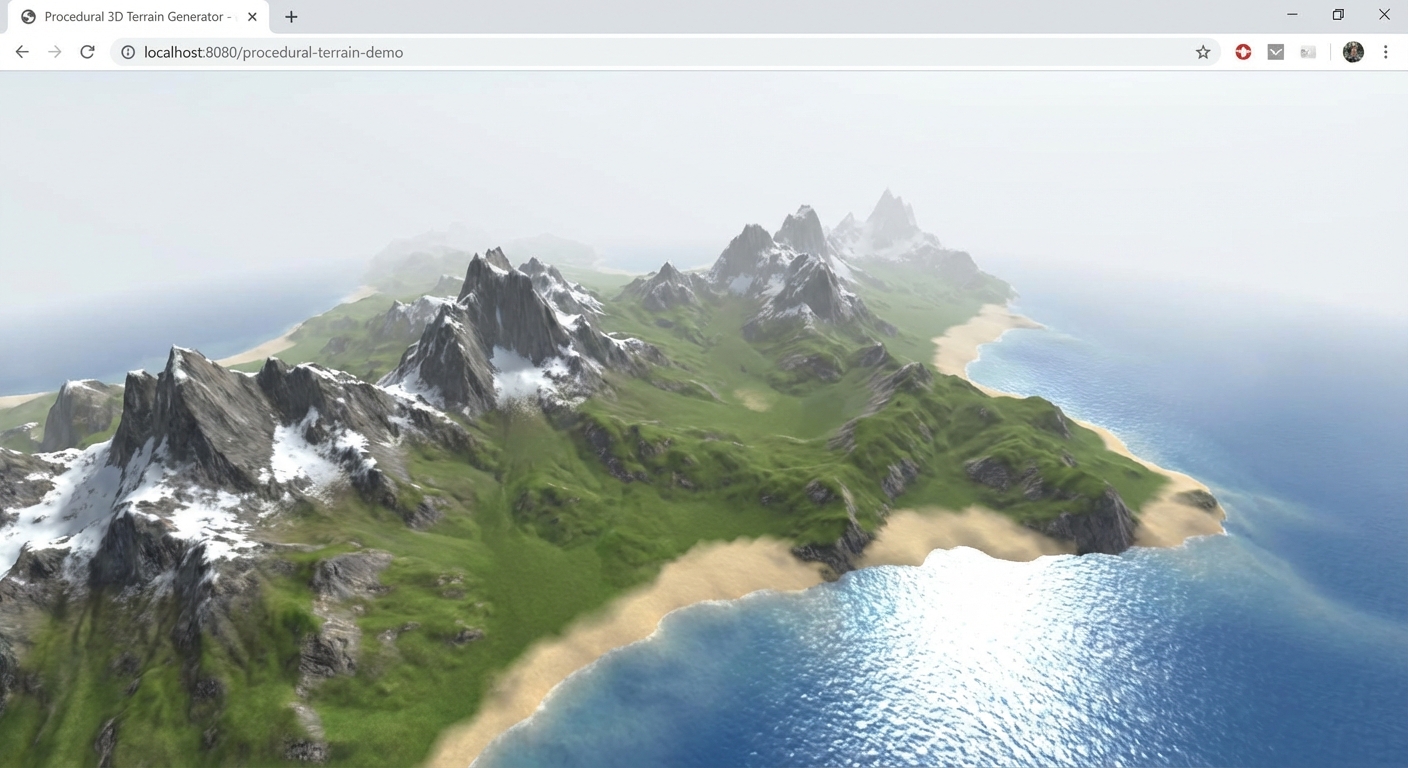
The Core Question You Are Answering
“How do noise functions, vertex displacement, and height-based shading work together to generate convincing natural terrain entirely from mathematics – no external assets required?”
This question matters because procedural generation is one of the most powerful techniques in computer graphics. Games like Minecraft, No Man’s Sky, and every terrain tool in Blender, Houdini, and Unreal Engine rely on the same noise-based principles you implement here. Understanding FBM, octaves, frequency, and amplitude gives you the mathematical vocabulary to generate any natural pattern: clouds, fire, water, wood grain, marble, mountains. This is the project where mathematics becomes visible.
Concepts You Must Understand First
- Noise Functions (Perlin, Simplex)
- What is the difference between random noise and coherent noise? Why does Perlin noise produce smooth, continuous values?
- Reference: “The Book of Shaders” - Ch. 10 (Random), Ch. 11 (Noise)
- Fractal Brownian Motion (FBM)
- How do you layer multiple octaves of noise at increasing frequencies and decreasing amplitudes to create natural complexity?
- Book Reference: “Math for Programmers” by Paul Orland - Ch. 2-3 (Vector math underpinning noise coordinates)
- Vertex Displacement
- How does the vertex shader modify the Y position of each vertex based on noise, and why must you also recalculate normals after displacement?
- Book Reference: “Computer Graphics from Scratch” by Gabriel Gambetta - Ch. 9 (Perspective Projection, vertex transformation)
- Height-Based Fragment Coloring
- How does the fragment shader determine color based on the interpolated height (varying) passed from the vertex shader?
- Reference: “The Book of Shaders” - Ch. 5 (Shaping Functions, smoothstep)
- Fog in Three.js
- How does
THREE.FogorTHREE.FogExp2blend distant fragments toward a fog color, and how does this interact with custom shaders? - Reference: Three.js docs - Fog, FogExp2
- How does
- PlaneGeometry Subdivision
- How do width and height segments in PlaneGeometry affect vertex density, and why does the vertex shader need enough vertices to produce smooth displacement?
- Reference: Three.js docs - PlaneGeometry
Questions to Guide Your Design
- Noise Implementation
- Do you compute noise on the CPU (JavaScript) and write to a height texture, or compute it in the vertex shader (GLSL)? What are the tradeoffs?
- CPU approach: Generate a heightmap as a texture, upload once, sample in vertex shader via
texture2D(). Pro: easy to debug (you can visualize the texture). Con: resolution limited by texture dimensions, updating requires re-uploading. - GPU approach: Compute noise directly in the vertex shader. Pro: infinite resolution, no texture memory, real-time parameter changes. Con: more expensive per-vertex computation, harder to debug.
- CPU approach: Generate a heightmap as a texture, upload once, sample in vertex shader via
- How do you include GLSL noise functions in your ShaderMaterial? (Inline strings, glslify, or manual inclusion?)
- Do you compute noise on the CPU (JavaScript) and write to a height texture, or compute it in the vertex shader (GLSL)? What are the tradeoffs?
- Terrain Tiling for Infinite Scrolling
- How do you create the illusion of infinite terrain? Do you use a single plane that scrolls its UV offset, or multiple tile planes that recycle?
- How do you ensure seamless transitions at tile boundaries?
- For the simple approach (single plane with scrolling noise), you offset the noise sampling coordinate by
uTime * speed. The terrain shape changes smoothly because noise is continuous.
- Normal Recalculation
- After displacing vertices in the vertex shader, the original flat normals are wrong. How do you compute new normals for correct lighting?
- Can you use finite differences (sample noise at neighboring points) to approximate the surface normal?
- The finite difference approach:
epsilon = 0.01 heightL = fbm(pos.xz + vec2(-epsilon, 0)) heightR = fbm(pos.xz + vec2(+epsilon, 0)) heightD = fbm(pos.xz + vec2(0, -epsilon)) heightU = fbm(pos.xz + vec2(0, +epsilon)) normal = normalize(vec3(heightL - heightR, 2.0 * epsilon, heightD - heightU)) - This samples noise 4 extra times per vertex (total 5x with the main sample), which costs performance but produces accurate normals.
- Water Rendering
- Should the water be a separate plane at a fixed Y level, or should it be part of the terrain shader?
- How do you make the water feel alive with animated normals and reflections?
- A separate plane is simpler and allows different material settings (high metalness, low roughness, blue tint, animated normal map).
- Performance Budget
- A 256x256 plane has 65,536 vertices. Each vertex runs the noise function (with 6 octaves, that is 6 noise evaluations per vertex, plus 4 more for normal reconstruction = 10 noise calls per vertex). Total: 655,360 noise function evaluations per frame. Modern GPUs handle this easily at 60fps.
- At what point do you need to consider LOD (fewer segments for distant terrain)?
- At 512x512 (262,144 vertices, 2.6M noise evaluations), you may start seeing frame drops on mobile. Consider using a texture-based approach or lower segment count for mobile.
Thinking Exercise
Exercise: Trace One Vertex Through the Shader Pipeline
Pick a single vertex at grid position (128, 128) on a 256x256 plane:
- Its original position is (0.0, 0.0, 0.0) in local space (center of the plane).
- The vertex shader receives this position as the
positionattribute. - You scale the XZ coordinates by the terrain scale uniform (e.g., multiply by 2.0) to get noise coordinates.
- You add a time-based offset to the Z coordinate for scrolling:
noiseCoord.y += uTime * speed. - You compute FBM noise at the scaled/offset coordinate: start with frequency = 1.0, amplitude = 1.0. For each octave, accumulate
amplitude * noise(frequency * coord), thenfrequency *= 2.0,amplitude *= 0.5. - The resulting noise value (e.g., 0.47) is multiplied by the height multiplier uniform (e.g., 10.0) to get the vertex Y displacement (4.7).
- You set
gl_Position = projectionMatrix * modelViewMatrix * vec4(pos.x, 4.7, pos.z, 1.0). - You pass the height (4.7) as a varying to the fragment shader.
- The fragment shader receives the interpolated height and applies the color band: 4.7 / 10.0 = 0.47, which falls in the “rocky terrain” band (0.35-0.65), so it outputs a gray-brown color.
FBM Octave Breakdown for this vertex:
Octave 1: freq=1.0, amp=1.0, noise(2.0, 2.0) = 0.32  -> contribution: 0.32
Octave 2: freq=2.0, amp=0.5, noise(4.0, 4.0) = 0.18  -> contribution: 0.09
Octave 3: freq=4.0, amp=0.25, noise(8.0, 8.0) = -0.1 -> contribution: -0.025
Octave 4: freq=8.0, amp=0.125, noise(16, 16) = 0.62   -> contribution: 0.078
Octave 5: freq=16, amp=0.0625, noise(32, 32) = -0.3   -> contribution: -0.019
Octave 6: freq=32, amp=0.03125, noise(64, 64) = 0.45  -> contribution: 0.014
                                                          ─────────────────
                                               Total FBM: 0.468
                                        x height (10.0): 4.68 units
Each octave adds finer detail at half the amplitude. Octave 1 creates large rolling hills. Octave 6 adds tiny bumps barely visible except up close.
Questions to answer:
- What happens if you use the same noise function for all octaves versus different noise functions for each? (Same function is standard – varying only frequency/amplitude creates the fractal structure. Different functions per octave would break the self-similar fractal property.)
- How does the terrain change if you use
amplitude *= 0.3instead ofamplitude *= 0.5for each octave? (Lower persistence (0.3) means higher octaves contribute much less, producing smoother terrain with less fine detail. Higher persistence (0.7) would make the terrain rough and jagged.) - If you skip the normal recalculation, what visual artifact will you see on the terrain? (The lighting will be flat and uniform – the terrain will look like a colored painting draped over bumps, with no shadows on slopes or highlights on ridges. The normals all point straight up regardless of surface angle.)
- What is the maximum possible height from this FBM configuration? (With 6 octaves and persistence 0.5: max = 1.0 + 0.5 + 0.25 + 0.125 + 0.0625 + 0.03125 = 1.96875. Multiplied by height 10.0 = 19.7 units. Actual values will be lower since noise rarely reaches +/-1.0 simultaneously across all octaves.)
The Interview Questions They Will Ask
- “Explain the difference between Perlin noise and white noise. Why is coherent noise essential for procedural terrain?”
- “What is Fractal Brownian Motion and how do octaves, frequency, and amplitude work together to create realistic terrain detail?”
- “You displaced vertices in the vertex shader but the lighting looks flat. What went wrong and how do you fix it?”
- “How would you implement infinite terrain scrolling without running out of memory or creating visible seams?”
- “What are the performance tradeoffs between computing heightmaps on the CPU versus the GPU vertex shader?”
- “How would you add biomes (desert, forest, tundra) to this terrain generator?”
Hints in Layers
Hint 1: Start With a Static Displaced Plane
Create a PlaneGeometry with 256x256 segments. Use a ShaderMaterial with a vertex shader that displaces the Y position using a simple sine wave: pos.y = sin(pos.x * 5.0) * cos(pos.z * 5.0) * 2.0. This verifies your shader pipeline works before you add noise complexity. Rotate the plane so Y is up (PlaneGeometry defaults to XY orientation; rotate -PI/2 on X).
Hint 2: Add Noise Functions
Find a GLSL Simplex noise implementation (search for “webgl-noise” by Ashima Arts or stegu). Paste the noise function code at the top of your vertex shader string. Replace the sine wave with snoise(pos.xz * uScale). Then build up FBM by calling the noise function in a loop, accumulating octaves with increasing frequency and decreasing amplitude.
Hint 3: Height-Based Coloring
Pass the displaced height as a varying from vertex to fragment shader. In the fragment shader, use smoothstep() to blend between color bands. Do not use hard if/else boundaries – smoothstep produces natural transitions. For example: mix(sandColor, grassColor, smoothstep(0.03, 0.08, height)).
Hint 4: Infinite Scrolling
Add a uTime uniform that increases each frame. In the vertex shader, offset the noise sampling coordinate by uTime * speed along one axis. The plane stays in place spatially, but the noise pattern slides through it, creating the illusion of forward motion. For true infinite terrain with tile recycling, use multiple plane chunks that reposition when they scroll past the camera.
Books That Will Help
| Topic | Book | Chapter |
|---|---|---|
| Noise functions and FBM | “The Book of Shaders” by Gonzalez Vivo | Ch. 10-11 (Random, Noise) |
| 3D vectors and coordinates | “Math for Programmers” by Paul Orland | Ch. 2-3 (2D/3D vectors) |
| Transformation matrices | “Math for Programmers” by Paul Orland | Ch. 4-5 (Transforms, Matrices) |
| Perspective projection | “Computer Graphics from Scratch” by Gabriel Gambetta | Ch. 9 (Perspective Projection) |
| Shading models | “Computer Graphics from Scratch” by Gabriel Gambetta | Ch. 13 (Shading) |
| Texture mapping concepts | “Computer Graphics from Scratch” by Gabriel Gambetta | Ch. 14 (Textures) |
Common Pitfalls and Debugging
Problem 1: “The terrain is completely flat – no displacement visible”
- Why: PlaneGeometry creates a plane in XY orientation by default. You need to rotate it by -Math.PI / 2 on the X axis so it lies flat with Y as the up axis. Alternatively, displace vertices along the Z axis in the vertex shader if the plane is in XZ orientation. Also check that your noise function is actually included in the shader string (GLSL compile errors are silent unless you check the console).
- Fix: Check the browser console for WebGL shader compilation errors. Log the shader source. Ensure the plane is oriented correctly.
- Quick test: Replace the noise displacement with a constant (e.g.,
pos.y += 5.0) to verify vertex displacement works at all.
Problem 2: “The terrain looks smooth and blobby, not detailed”
- Why: You are using only 1-2 octaves of noise. Real terrain needs 4-8 octaves of FBM for fine detail (ridges, crevices, small bumps).
- Fix: Increase the octave count and ensure each octave doubles the frequency and halves the amplitude. Also ensure your plane has enough vertex segments – 64x64 might not be enough for fine noise detail. Try 256x256 or 512x512.
- Quick test: Add a lil-gui slider for octave count (1-8) and watch the terrain complexity change in real-time.
Problem 3: “Lighting is wrong – the terrain appears uniformly lit with no shadows on slopes”
- Why: After displacing vertices in the vertex shader, the original flat normals are no longer correct. The normals still point straight up even though the surface is now bumpy.
- Fix: Recalculate normals in the vertex shader using finite differences: sample the noise at two nearby points (offset by a small epsilon in X and Z), compute the tangent and bitangent vectors, and take their cross product to get the new normal. Pass this recalculated normal to the fragment shader.
- Quick test: Temporarily output the normal as the fragment color (
gl_FragColor = vec4(vNormal * 0.5 + 0.5, 1.0)) to visualize whether normals vary across the surface.
Problem 4: “Visible seams or jumps when terrain tiles recycle”
- Why: If you use a tile-based infinite scrolling approach, the noise values at tile edges do not match because each tile samples noise at different coordinates.
- Fix: Ensure tiles sample noise using world-space coordinates (not local UV coordinates). When a tile recycles from the front to the back, its vertices should sample noise at the correct world-space position. The noise function itself is continuous, so if you feed it continuous coordinates, the output will be seamless.
- Quick test: Place two tiles side by side and check whether the terrain height matches exactly at the boundary.
Definition of Done
- A subdivided plane (minimum 256x256 segments) is displaced by FBM noise in the vertex shader
- Height-based coloring with smooth transitions: sand, grass, rock, and snow bands are visible
- The terrain scrolls continuously to create the illusion of flight over infinite landscape
- A water plane sits at an adjustable sea level with some reflective/transparent appearance
- Fog fades distant terrain into a sky-colored background
- lil-gui controls are functional: terrain scale, height multiplier, water level, fog density, octave count, speed
- Normals are recalculated after vertex displacement so lighting is correct on slopes
- A DirectionalLight and HemisphereLight provide realistic terrain lighting
- Performance stays above 30fps on a mid-range device
- The terrain has no visible seams or tiling artifacts
Project 10: First-Person 3D Environment
- File: P10-first-person-environment.md
- Main Programming Language: JavaScript
- Alternative Programming Languages: TypeScript, Kotlin/JS
- Coolness Level: 4 - Impressive (People lean in when they see it)
- Business Potential: 2 - Niche (Useful in specific domains)
- Difficulty: Advanced
- Knowledge Area: First-Person Controls / Level Design / Collision
- Software or Tool: Three.js, PointerLockControls, GLTFLoader, DRACOLoader, lil-gui
- Main Book: “Computer Graphics from Scratch” by Gabriel Gambetta - Ch. 9-10 (Perspective Projection, Scene Description)
What you will build: A walkable first-person 3D environment – a virtual museum, apartment, or sci-fi corridor – where the player navigates with WASD keys and mouse look. The environment is loaded from a GLTF model. Doors open on approach, lights toggle when clicking switches, and the player cannot walk through walls.
Why it teaches Three.js: First-person environments combine nearly every Three.js skill: loading complex 3D assets (GLTF), managing camera controls (PointerLockControls), implementing collision detection (raycasting against environment geometry), handling user input (keyboard + mouse), and creating interactive objects (raycasting for clicks). This is the project where Three.js stops feeling like a toy and starts feeling like a game engine.
Core challenges you will face:
- PointerLockControls and Input Handling -> Maps to concept: Camera Systems / Controls
- GLTF Scene Loading and Traversal -> Maps to concept: Asset Loading
- Basic Collision Detection -> Maps to concept: Raycasting / Physics
- Interactive Objects (click to activate) -> Maps to concept: Raycasting and Interactivity
- Environment Lighting and Atmosphere -> Maps to concept: Lighting and Shadows
Real World Outcome
When you open the browser, you see a landing screen overlay with centered text: “Click to Enter.” The 3D environment is visible but blurred behind the overlay. Clicking anywhere triggers PointerLockControls.lock(), which captures the mouse cursor and hides it. The overlay fades out, and you are now standing inside a 3D environment in first-person view.
The Environment is loaded from a GLTF/GLB model. You can create it in Blender or download a free model from Sketchfab or similar sources. The environment could be:
- A small museum with 3 rooms connected by doorways, art on the walls, spotlights on each piece
- A sci-fi corridor with metallic walls, glowing panels, and sliding doors
- A modern apartment with furniture, windows, and kitchen
The camera is positioned at eye height (Y = 1.6 units, assuming 1 unit = 1 meter). Looking around is smooth and responsive – moving the mouse rotates the camera view naturally. There is no cursor visible; the mouse is locked.
Movement: Pressing W moves forward in the direction you are looking. S moves backward. A strafes left, D strafes right. Movement speed is consistent (e.g., 5 units/second, adjusted by delta time). There is no vertical movement – the player stays at ground level.
Collision Detection: You cannot walk through walls, furniture, or closed doors. As you approach a wall, movement stops in that direction. This is implemented using raycasting: before moving, cast rays in the movement direction from the player’s position. If a ray intersects a wall mesh within a short distance (e.g., 0.5 units), movement in that direction is blocked. Multiple rays are cast (forward, left, right, backward relative to movement direction) for smooth collision response.
Interactive Objects:
- Doors: When you walk within 2 meters of a door, it smoothly swings open (rotation animation on the Y axis over 0.8 seconds). When you walk away, it closes. The door’s pivot point must be at its hinge edge, not its center.
- Light Switches: Small box meshes on walls. A crosshair (small white dot or cross) is always visible at the center of the screen. When the crosshair points at a light switch and you click (left mouse button), the associated light toggles on/off. The switch visually flips (rotation animation), and the nearby light source (PointLight or SpotLight) enables/disables. When the light is off, that area of the room darkens realistically.
- Information Panels (optional): Clickable plaques next to art pieces that display HTML overlay text when clicked.
Visual Details: The environment uses baked lightmaps for base illumination (embedded in the GLTF from Blender) supplemented by real-time lights for the interactive switches. Shadows are enabled for at least one directional or spot light. The floor has a subtle normal map for surface detail. Environmental fog adds depth to longer corridors.
HUD Elements: A small white crosshair (CSS element) is fixed at the center of the viewport. When the crosshair hovers over an interactive object (detected by continuous raycasting from camera center), the crosshair changes color (e.g., white to green) to indicate interactability.
When you press Escape, the pointer lock releases, the mouse cursor reappears, and a pause menu overlay appears with “Resume” and “Controls” options.
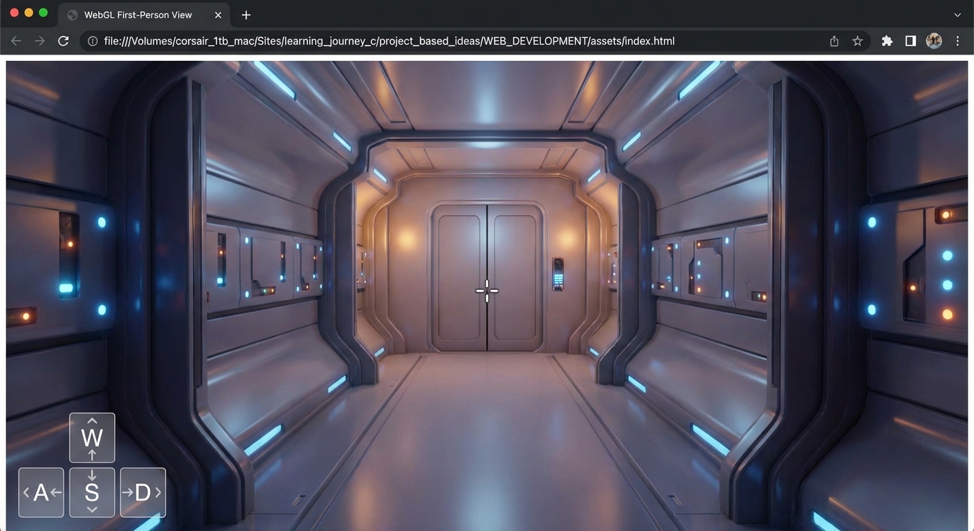
The Core Question You Are Answering
“How do you combine asset loading, first-person camera controls, collision detection, and interactive objects to create a walkable 3D environment that feels responsive and physically grounded?”
This question matters because walkable 3D environments are the foundation of games, virtual tours, architectural visualization, training simulations, and metaverse experiences. The specific combination of pointer lock controls, GLTF loading, collision raycasting, and interactive objects covers the full stack of skills needed to build any first-person web experience. Understanding these systems together (not in isolation) is what separates demo projects from real applications.
Concepts You Must Understand First
- PointerLockControls
- How does the Pointer Lock API capture and hide the mouse cursor, and how does PointerLockControls translate mouse movement into camera rotation?
- Reference: Three.js docs - PointerLockControls, MDN - Pointer Lock API
- GLTF Scene Loading and Traversal
- How do you load a GLTF model, traverse its scene graph to find specific objects by name, and enable shadows on meshes?
- Book Reference: “Computer Graphics from Scratch” by Gabriel Gambetta - Ch. 10 (Describing and Rendering a Scene)
- Raycasting for Collision Detection
- How do you cast rays from the player position in the movement direction to detect walls before the player reaches them?
- Reference: Three.js docs - Raycaster, Discover Three.js - Raycasting chapter
- Raycasting for Object Interaction
- How do you cast a ray from the camera center (screen center) forward to detect which object the player is looking at?
- Reference: Three.js docs - Raycaster.setFromCamera
- Delta-Time Movement
- Why must movement speed be multiplied by delta time, and what happens if you do not?
- Reference: Discover Three.js - Animation Loop chapter
- Environment Lighting
- How do you combine baked lightmaps (from GLTF) with real-time dynamic lights for interactive elements?
- Reference: Three.js docs - LightMap, SpotLight, PointLight
Questions to Guide Your Design
- Collision Architecture
- Do you cast one ray or multiple rays from the player? One ray only checks directly ahead – the player can clip corners. Multiple rays (e.g., 8 evenly spaced around the player) provide better collision at higher cost.
- Should you separate collision geometry from visual geometry? (Simplified invisible collision meshes vs raycasting against the full GLTF model)
- Object Naming Convention
- How do you identify interactive objects in the loaded GLTF? By name prefix (e.g., “door_01”, “switch_kitchen”), by userData, or by a separate manifest?
- How do you associate a light switch with the light it controls?
- Door Animation
- How do you animate a door opening? The pivot must be at the hinge, not the center. Do you parent the door mesh to an empty Object3D at the hinge position and rotate the parent?
- How do you trigger the animation only once when approaching, and reverse it when leaving?
- Performance with Complex GLTF Models
- A detailed environment might have hundreds of meshes. How do you optimize raycasting to not test against every mesh?
- Should you create simplified collision geometry (invisible boxes/planes) separate from the visual meshes?
- Mobile / Fallback
- Pointer Lock is a desktop-only API. How would you handle touch input on mobile devices as a fallback?
- What happens if the browser does not support Pointer Lock?
Thinking Exercise
Exercise: Design the Collision System
Map out the collision detection flow for a single frame where the player presses W (forward):
Frame Start
    |
    v
Read Input -> W key is pressed
    |
    v
Get camera forward direction:
    forward = camera.getWorldDirection(tempVec)
    forward.y = 0       // Zero out vertical component
    forward.normalize()  // Re-normalize after zeroing Y
    |
    v
Calculate desired displacement:
    displacement = forward * speed * deltaTime
    (e.g., forward * 5.0 * 0.016 = 0.08 units this frame)
    |
    v
Cast collision rays (4 rays minimum):
    Ray 1: from playerPos, direction = forward, far = 0.5
    Ray 2: from playerPos + rightOffset, direction = forward, far = 0.5
    Ray 3: from playerPos - rightOffset, direction = forward, far = 0.5
    Ray 4: from playerPos + Vector3(0, -0.5, 0), direction = forward, far = 0.5
    |
    v
Check intersections:
    intersections = raycaster.intersectObjects(collidables)
    |
    +---> No intersection: Apply full displacement
    |         camera.position.add(displacement)
    |
    +---> Intersection detected at distance < buffer:
              Option A: Block movement (stop dead)
              Option B: Slide along wall:
                  wallNormal = intersection.face.normal
                  slideDir = displacement - wallNormal * dot(displacement, wallNormal)
                  camera.position.add(slideDir)
    |
    v
Lock Y position:
    camera.position.y = EYE_HEIGHT  // Always 1.6
    |
    v
Render frame
Questions to answer:
- What happens if you only cast one ray from the center of the player? (The player’s “body” has width. A single center ray misses walls that are to the left or right of center. The player can clip through wall corners because the center ray passes beside the corner while the player’s “shoulder” would hit it.)
- How would you handle stairs or ramps? (Cast a ray downward from the new position. If the ground intersection is slightly higher than the current Y (within a step height threshold like 0.3 units), raise the player smoothly. If the ground drops away (more than step height), either fall or prevent movement.)
- What is the difference between blocking movement and sliding along a wall? Which feels better to the player? (Blocking stops the player dead, which feels frustrating – like hitting a wall of glue. Sliding projects the movement onto the wall’s tangent plane so the player glides along walls, which feels natural and responsive. Sliding is always preferred in first-person games.)
- Why do you zero out the Y component of the forward direction? (Without zeroing Y, looking up and pressing W would make the player fly upward. Looking down would push them into the floor. FPS movement should always be horizontal regardless of where the camera points.)
The Interview Questions They Will Ask
- “How does the Pointer Lock API work, and how does Three.js PointerLockControls use it to create first-person camera control?”
- “Describe how you would implement collision detection for a first-person character in Three.js without using a physics engine.”
- “You loaded a GLTF model of a building. How do you identify and interact with specific objects like doors and switches?”
- “What is the difference between raycasting against visual meshes and raycasting against simplified collision geometry? When would you choose each approach?”
- “How do you handle the case where the player walks into a corner formed by two walls meeting at a right angle? How do you prevent the player from getting stuck?”
Hints in Layers
Hint 1: Basic FPS Setup Start with an empty scene (no GLTF). Add a floor plane, a few box geometries for walls, and PointerLockControls. Implement WASD movement using keyboard event listeners that set velocity direction flags. In the animation loop, apply velocity * delta to the camera position. Get basic mouse look and walking working before adding any complexity.
Hint 2: Add Collision
Create an array of “collidable” meshes (your wall boxes). Before applying movement, cast a Raycaster from the camera position in the movement direction. If raycaster.intersectObjects(collidables) returns an intersection with distance less than your buffer, block that movement component. Cast separate rays for forward/backward and left/right to allow sliding along walls.
Hint 3: Load the GLTF Environment
Replace your box walls with a GLTF model. After loading, traverse the scene to find all meshes: gltf.scene.traverse(child => { if(child.isMesh) collidables.push(child) }). Enable shadows with child.castShadow = true; child.receiveShadow = true. Name objects in Blender with a convention like “wall_” for collision and “door_” for interactive doors.
Hint 4: Interactive Objects
In the animation loop, cast a ray from the camera center (0, 0 in NDC) forward using raycaster.setFromCamera({x: 0, y: 0}, camera). Check if the intersection is with an object whose name starts with “switch_”. If so, change the crosshair color. On click, toggle the associated PointLight’s visible property and animate the switch mesh rotation.
Books That Will Help
| Topic | Book | Chapter |
|---|---|---|
| Scene description and rendering | “Computer Graphics from Scratch” by Gabriel Gambetta | Ch. 9-10 (Projection, Scene Description) |
| Hidden surface removal (depth) | “Computer Graphics from Scratch” by Gabriel Gambetta | Ch. 12 (Hidden Surface Removal) |
| 3D coordinate systems | “Math for Programmers” by Paul Orland | Ch. 3 (Ascending to 3D) |
| Vector math for movement | “Math for Programmers” by Paul Orland | Ch. 2-3 (2D/3D Vectors) |
| Transformation for door pivots | “Math for Programmers” by Paul Orland | Ch. 4-5 (Transforms, Matrices) |
Common Pitfalls and Debugging
Problem 1: “The player falls through the floor or floats above it”
- Why: PointerLockControls does not lock the Y position. Any vertical component in the camera’s forward direction causes the player to drift up or down.
- Fix: After applying movement, force the camera’s Y position to a constant eye height:
camera.position.y = 1.6. Or zero out the Y component of the movement vector before applying it. - Quick test: Look straight up and walk forward. If the player rises, Y is not being locked.
Problem 2: “Collision detection fails on thin walls – the player passes through”
- Why: If the player moves fast enough (or delta time spikes), the movement distance per frame exceeds the wall thickness. The ray starts before the wall and the new position is past it (tunneling).
- Fix: Cap the maximum movement distance per frame. Or use continuous collision detection: cast the ray with
farset to the movement distance + buffer, and only move up to the intersection point minus the buffer. - Quick test: Increase movement speed to 50 and try walking through walls.
Problem 3: “The GLTF model is enormous or tiny when loaded”
- Why: GLTF models have their own scale. A model created in Blender at real-world scale (1 unit = 1 meter) should work, but some models use centimeters or arbitrary units.
- Fix: After loading, check the model’s bounding box:
new THREE.Box3().setFromObject(gltf.scene). If the dimensions are wrong, scale the root:gltf.scene.scale.set(0.01, 0.01, 0.01)for a model in centimeters. - Quick test: Add a 1x1x1 box at the origin as a reference cube. Is it roughly the size of a 1-meter cube relative to the loaded model?
Problem 4: “Doors rotate around their center instead of their hinge”
- Why: Mesh pivot points default to the geometry’s center. A door mesh rotates around its center, not its edge.
- Fix: In Blender, move the origin (pivot point) of the door mesh to the hinge edge before exporting. In Three.js, you can work around this by creating an empty Group at the hinge position, parenting the door mesh to it with an offset, and rotating the Group.
- Quick test: Create a box and rotate it on Y. Observe it spinning around its center. Then parent it to a Group at one edge and rotate the Group.
Definition of Done
- PointerLockControls captures the mouse on click, releases on Escape
- WASD movement works with delta-time-adjusted speed
- Camera is locked to eye height (no flying or falling)
- A 3D environment is loaded from a GLTF/GLB file
- The player cannot walk through walls (raycast collision detection)
- At least one door opens and closes based on player proximity
- At least one light switch toggles a light on/off when clicked
- A crosshair at screen center changes color when pointing at an interactive object
- Escape shows a pause overlay with pointer lock release
- The environment has functional lighting (at least one shadow-casting light)
Project 11: Particle System Showcase
- File: P11-particle-system-showcase.md
- Main Programming Language: JavaScript + GLSL
- Alternative Programming Languages: TypeScript, Rust (WASM for compute)
- Coolness Level: 5 - Mind-Blowing (They want to know how you did it)
- Business Potential: 1 - Learning Only (Pure learning project)
- Difficulty: Advanced
- Knowledge Area: Particles / GPU Programming / Visual Effects
- Software or Tool: Three.js, THREE.Points, ShaderMaterial, BufferGeometry, lil-gui
- Main Book: “Math for Programmers” by Paul Orland - Ch. 2-5 (Vectors, Transforms, Matrices)
What you will build: Four distinct particle effects showcased as a switchable gallery: a campfire with fire, sparks, and smoke layers; a rain storm with falling streaks and ground splashes; a spiral galaxy of orbiting stars; and text that dissolves into particles that drift away. A tab bar at the top switches between effects.
Why it teaches Three.js: Particle systems demand mastery of GPU programming. You will write custom vertex and fragment shaders, manage thousands of per-particle attributes (position, velocity, lifetime, color, size) in BufferGeometry, use additive blending and depth tricks, and animate everything on the GPU for maximum performance. Each of the four effects teaches a different particle behavior pattern: emitters, physics simulation, orbital motion, and geometry-to-particle conversion.
Core challenges you will face:
- Custom Particle Shaders -> Maps to concept: Shaders and GLSL
- Per-Particle Attributes in BufferGeometry -> Maps to concept: Geometry / BufferAttributes
- GPU-Based Animation -> Maps to concept: Animation Loop / Performance
- Additive Blending and Transparency -> Maps to concept: Materials / Blending
- Sprite Textures and Point Rendering -> Maps to concept: Textures / Particles
Real World Outcome
When you open the browser, you see a horizontal tab bar at the top of the viewport with four tabs: “Campfire,” “Rain Storm,” “Galaxy,” and “Text Dissolve.” The currently selected tab is highlighted. The rest of the viewport shows the active particle effect against a dark background.
Effect 1: Campfire
A realistic campfire burns at the center of the scene. The effect consists of three separate particle systems layered together:
-
Fire particles (~500 particles): Orange and yellow points that spawn at the base of the fire (a small area at the origin) and rise upward with slight horizontal turbulence. Each particle starts large and bright at the bottom, shrinks and fades to transparent as it rises, and disappears after ~1 second. The particles use additive blending, so overlapping particles create brighter regions. The overall shape is a cone of fire tapering upward. A soft circular sprite texture gives each particle a round, glowing appearance.
-
Sparks (~200 particles): Tiny bright white-yellow points that launch upward from the fire at higher velocity than the flames. They follow slight parabolic arcs (gravity pulling them back down), flickering rapidly. Some sparks drift sideways in the wind. They are smaller and brighter than fire particles, creating the characteristic sparkle of a real campfire.
-
Smoke (~300 particles): Large, semi-transparent dark gray particles that spawn above the fire and drift upward slowly, expanding in size as they rise. They use normal (not additive) blending with low opacity (~0.1-0.2). They billow and sway with Perlin noise-based turbulence. They are the slowest and longest-lived particles, fading out after 3-5 seconds at a height well above the flames.
Below the fire, a few log meshes (simple cylinder geometries with brown MeshStandardMaterial, roughness 0.9) sit in a crossed arrangement, glowing faintly orange from a PointLight positioned at the fire’s base. The PointLight has a warm orange color (#FF6600), intensity of 2.0, and a decay of 2.0, creating a realistic falloff. The light flickers slightly by randomizing its intensity between 1.5 and 2.5 each frame using light.intensity = 2.0 + Math.sin(time * 15) * 0.3 + Math.random() * 0.2. This subtle intensity variation makes the light feel alive and organic, casting dancing shadows on the ground around the fire.
A dark ground plane extends beneath the fire with a MeshStandardMaterial (dark brown, roughness 0.8) that catches the flickering light. The combination of the three particle layers (fire + sparks + smoke) with the flickering point light creates a convincing campfire scene despite using no textures for the particles themselves.
Effect 2: Rain Storm
Thousands of white elongated particles (~5,000) fall downward from a spawning plane positioned above and around the camera. Each rain particle is not a dot but a short vertical streak – this is achieved in the vertex shader by rendering each point as a tall rectangle (using gl_PointSize with an aspect ratio trick, or by stretching the sprite texture vertically). The streak length is proportional to the particle’s falling speed, creating motion blur. The streaks move quickly (Y velocity of -8 to -12 units/second), creating the visual impression of heavy rainfall.
Each rain particle spawns at a random XZ position within a 20x20 unit area centered on the camera, at a Y height of 10. It falls straight down. When its Y position goes below 0 (the ground), it wraps back to Y = 10 with a new random XZ position (handled in the vertex shader using mod()).
When rain particles hit the ground plane (Y = 0), small splash particles (~1,000) burst outward in tiny rings at the impact points. Each splash is a set of 4-8 tiny particles that shoot outward horizontally at the impact XZ coordinate, decelerate quickly, and fade out within 0.2 seconds. The splashes use normal blending (not additive) with low opacity.
The ground plane itself is a dark, slightly reflective surface (MeshStandardMaterial with roughness 0.3 and metalness 0.1) that catches the rain reflections. A thin layer of animated water ripples (normal map animation) covers the ground.
The scene is dark and moody with a slight blue-gray ambient light (HemisphereLight with sky color #334466 and ground color #111111). Dense fog (FogExp2 with density 0.08) reduces visibility to a few meters, making distant rain fade into gray. Occasional lightning is simulated by briefly flashing the ambient light to white (every 5-10 seconds, with a random delay). When lightning triggers: the ambient light intensity spikes to 5.0 for 100ms, then decays over 300ms, creating a flash-then-fade effect. Optionally, a subtle screen shake (camera position oscillation for 200ms) accompanies the lightning.
Effect 3: Galaxy
A spiral galaxy fills the viewport. Approximately 50,000-100,000 star particles orbit around a bright central core. The stars are arranged in two or three spiral arms using a logarithmic spiral formula. Stars closer to the center orbit faster, creating differential rotation visible as the galaxy slowly spins.
Star colors vary: the core glows bright white-yellow, spiral arm stars are blue-white, and scattered halo stars are dimmer reddish tones. Each star has a size that varies with distance from the center (larger near core, smaller in the halo). The entire galaxy slowly rotates, with the spiral arms trailing behind due to differential rotation.
A subtle glow (bloom post-processing or additive blending) makes the core area intensely bright. Faint dust lanes (dark regions between spiral arms) are suggested by reduced particle density in certain angular ranges.
The galaxy’s structure follows real astrophysics:
- Core bulge: A dense concentration of ~10,000 particles within 20% of the galaxy radius, with random 3D distribution (not flat). These particles are the brightest and largest.
- Spiral arms: 2-3 arms containing ~30,000 particles each, following a logarithmic spiral. The arm width increases with radius (tighter near center, wider at edges).
- Halo: ~10,000 sparse particles distributed in a spherical shell around the entire galaxy, with dim red colors and small sizes. These represent old, distant stars.
- Differential rotation: Inner particles orbit with period T proportional to r^1.5 (Kepler’s third law). A star at radius 1 completes a full orbit in 10 seconds; a star at radius 4 takes 80 seconds. This creates the winding spiral pattern over time.
Effect 4: Text Dissolve
The word “THREE.JS” (or any text) is rendered as particles. Initially, the text is static and readable – thousands of small white particles are positioned to form the letter shapes. Then, on clicking a “Dissolve” button, the particles break apart: each particle receives a random velocity direction and begins drifting outward from its original position. Particles spin, fade, shrink, and scatter like dust blown from a surface.
After scattering fully (2-3 seconds), clicking “Reassemble” reverses the animation: particles smoothly return to their original text positions, like a video played in reverse. The text re-forms letter by letter from left to right.
The text particle positions are generated by rendering the text to a hidden 2D canvas (offscreen), reading the pixel data with getImageData(), and creating a particle at each opaque pixel’s position. The 2D canvas coordinates (in pixels) are mapped to 3D world coordinates:
- Canvas pixel (px, py) maps to 3D position:
x = (px - canvasWidth/2) * scale,y = (canvasHeight/2 - py) * scale,z = 0 - The scale factor determines the world-space size of the text (e.g., 0.05 maps a 200px-wide canvas to 10 world units)
- Transparent pixels (alpha < 128) are skipped, creating particles only where the text’s letterforms exist
The text uses a bold, wide font (e.g., Impact, Arial Black) at a large canvas font size (80-120px) to maximize the number of opaque pixels and therefore particles. A 400x100 canvas with 80px text typically produces 5,000-15,000 particle positions depending on the font.
A lil-gui panel (visible across all effects) controls: particle count multiplier, animation speed, and effect-specific parameters (fire height, rain intensity, galaxy arm count, dissolve force).

The Core Question You Are Answering
“How do you manage thousands of individual elements with per-particle state (position, velocity, lifetime, color, size) entirely on the GPU, and how do different particle behaviors (emitters, physics, orbits, morphing) map to different shader strategies?”
This question matters because particle systems are everywhere: game VFX, movie effects, scientific visualization, data art, and interactive installations. The techniques here – per-vertex attributes in BufferGeometry, GPU animation via vertex shaders, additive blending, and sprite texturing – are the foundation of all real-time visual effects. Understanding how to animate 100,000 elements at 60fps by moving computation from CPU to GPU is a skill that transfers to any performance-critical rendering task.
Concepts You Must Understand First
- THREE.Points and PointsMaterial
- How does THREE.Points render each vertex as a screen-facing sprite? How does
gl_PointSizecontrol the size of each point? - Reference: Three.js docs - Points, PointsMaterial
- How does THREE.Points render each vertex as a screen-facing sprite? How does
- Custom BufferAttributes
- How do you add per-particle data (velocity, lifetime, startTime, color) as custom BufferAttributes and access them in the vertex shader?
- Reference: Three.js docs - BufferGeometry, BufferAttribute
- GPU-Based Animation with Uniforms
- How do you pass elapsed time as a uniform and compute particle positions in the vertex shader instead of updating positions on the CPU?
- Reference: “The Book of Shaders” - Uniforms
- Additive Blending and depthWrite
- Why do particle systems use
AdditiveBlendinganddepthWrite: false? What visual artifacts occur without these settings? - Reference: Three.js docs - Material.blending, Material.depthWrite
- Why do particle systems use
- Sprite Textures for Particles
- How do you apply a circular gradient texture to points so they appear as soft glowing dots instead of hard squares?
- Reference: Three.js docs - PointsMaterial.map
- GLSL Math Functions
- What do
fract(),mod(),smoothstep(),mix(), andsin()/cos()do, and how are they used for particle animation? - Reference: “The Book of Shaders” - Ch. 5 (Shaping Functions)
- What do
Questions to Guide Your Design
- Particle Lifecycle Management
- How do you handle particle birth and death without creating/destroying BufferAttributes? (Hint: all particles exist always; “dead” particles are invisible or repositioned.)
- How do you implement particle respawning in the shader using
mod(uTime - startTime, lifetime)?
- Multiple Particle Systems per Effect
- The campfire has three separate particle systems (fire, sparks, smoke). Should these be three separate Points objects or one system with per-particle type flags?
- What are the tradeoffs of each approach?
- Text to Particles Conversion
- How do you render text to a 2D canvas, read pixel data with
getImageData(), and convert opaque pixel coordinates to 3D particle positions? - How do you handle text of varying lengths and fonts?
- How do you render text to a 2D canvas, read pixel data with
- Spiral Galaxy Math
- How do you position particles along logarithmic spiral arms? What formula produces a spiral in polar coordinates?
- How do you make inner particles orbit faster than outer particles (Keplerian rotation)?
- Performance at Scale
- At 100,000 particles, can you still animate on the CPU? (No – updating 100,000 positions in JavaScript at 60fps means 6 million position writes per second. The GPU can process all 100,000 vertices in parallel.)
- How do you structure the vertex shader to compute position from initial conditions + time rather than storing mutable state?
- What is the difference between “stateless” GPU particles (position = f(initialState, time)) and “stateful” CPU particles (position += velocity * dt)?
- Effect Switching
- When switching tabs, do you dispose old particle systems and create new ones, or do you keep all four loaded and toggle visibility?
- What is the memory implication of keeping 200,000 particles across four systems loaded simultaneously?
- How do you handle the transition animation between effects? (Cross-fade? Instant switch? Particle morph?)
Thinking Exercise
Exercise: Design the Campfire Particle Lifecycle
For the fire particle system (500 particles), design the complete lifecycle:
- Initialization (CPU, once):
- For each particle i (0 to 499), generate random attributes:
startTime[i]= random value in [0, maxLifetime] (stagger births so not all particles spawn simultaneously)initialPosition[i]= random position within a small disk at the fire base (x: [-0.3, 0.3], y: 0, z: [-0.3, 0.3])velocity[i]= upward direction with turbulence (x: [-0.2, 0.2], y: [1.0, 2.0], z: [-0.2, 0.2])lifetime[i]= random value in [0.5, 1.5] seconds
- Store all as BufferAttributes on the geometry.
- For each particle i (0 to 499), generate random attributes:
- Animation (GPU, every frame):
- Vertex shader receives
uTimeuniform. - Compute particle age:
age = mod(uTime - aStartTime, aLifetime) - Compute normalized age (0 to 1):
t = age / aLifetime - Compute current position:
pos = aInitialPos + aVelocity * age + turbulence(uTime) - Compute size:
gl_PointSize = mix(maxSize, 0.0, t)(shrinks over lifetime) - Pass
tas a varying to the fragment shader for color/opacity.
- Vertex shader receives
- Coloring (GPU, per pixel):
- Fragment shader receives normalized age
t. - Color:
mix(brightYellow, deepRed, t)– yellow at birth, red at death. - Opacity:
1.0 - t– fully opaque at birth, transparent at death. - Apply circular sprite mask using distance from point center:
if(distance(gl_PointCoord, vec2(0.5)) > 0.5) discard;
- Fragment shader receives normalized age
Questions to answer:
- Why use
mod(uTime - startTime, lifetime)instead of tracking absolute age? (mod()automatically wraps the age back to 0 when it exceeds the lifetime, causing the particle to “respawn” at its initial position. This means the CPU never needs to track particle state or reset buffers. The GPU handles all lifecycle management through pure math.) - What visual artifact occurs if all 500 particles have the same startTime? (All particles spawn, rise, and die simultaneously, creating a pulsing “pop” effect every lifetime interval. The fire appears to flash on and off instead of burning continuously. Staggered start times ensure particles are always at different lifecycle stages.)
- How would you add wind that pushes particles to the right? (Add a wind uniform
vec3 uWind = vec3(0.5, 0.0, 0.0). In the position computation, adduWind * age * agefor accelerating wind effect, oruWind * agefor constant wind. Multiply by a noise function for turbulent gusts:uWind * age * (1.0 + 0.3 * snoise(vec2(uTime, float(particleId)))))
Bonus: Trace through the fragment shader for a mid-life fire particle:
Input: t = 0.5 (halfway through life)

Step 1: Compute color
  brightYellow = vec3(1.0, 0.95, 0.2)
  deepRed = vec3(0.8, 0.1, 0.0)
  color = mix(brightYellow, deepRed, 0.5) = vec3(0.9, 0.525, 0.1)
  Result: warm orange

Step 2: Compute opacity
  alpha = 1.0 - t = 0.5 (semi-transparent)

Step 3: Apply sprite mask
  fragCoord = gl_PointCoord  // (0,0) top-left to (1,1) bottom-right
  dist = distance(fragCoord, vec2(0.5, 0.5))
  if dist > 0.5: discard  // outside circle
  // Optional: soft falloff
  alpha *= smoothstep(0.5, 0.2, dist)

Step 4: Output
  gl_FragColor = vec4(0.9, 0.525, 0.1, 0.5 * softEdge)
  With AdditiveBlending: this adds to whatever is behind it
The Interview Questions They Will Ask
- “How would you render 100,000 animated particles at 60fps in the browser? Describe the architecture.”
- “What is the difference between animating particles on the CPU (updating positions in JavaScript) versus the GPU (computing positions in the vertex shader)?”
- “How do you handle particle birth and death without dynamically resizing buffers?”
- “Explain additive blending. Why is it used for fire and energy effects but not for smoke?”
- “How would you convert 2D text into 3D particle positions for a text dissolve effect?”
- “What is
gl_PointCoordand how do you use it to apply circular textures to point sprites?”
Hints in Layers
Hint 1: Start With Static Points Create a BufferGeometry with 1,000 random positions. Wrap it in a Points object with a white PointsMaterial. Verify you see 1,000 white dots scattered in space. This confirms your Points pipeline works before adding complexity.
Hint 2: Add Motion with a Shader
Replace PointsMaterial with a ShaderMaterial. In the vertex shader, add uniform float uTime and offset the Y position: pos.y += uTime * aVelocity.y. Pass uTime from JavaScript each frame. The particles should now drift upward continuously. Use mod() to wrap the Y position back to the start for looping.
Hint 3: Add Lifecycle (Birth/Death)
Add aStartTime and aLifetime attributes. In the vertex shader, compute age = mod(uTime - aStartTime, aLifetime) and normalized age t = age / aLifetime. Set gl_PointSize = mix(20.0, 0.0, t) so particles shrink to nothing at death and reappear large at birth. Pass t to the fragment shader for opacity: gl_FragColor.a = 1.0 - t.
Hint 4: Polish With Textures and Blending
Load a circular gradient texture (white center fading to transparent edges). Set it as the Points material’s map. Enable transparent: true, blending: THREE.AdditiveBlending, and depthWrite: false. In the fragment shader, discard fragments beyond the circle radius using gl_PointCoord. The particles should now look like soft glowing orbs instead of squares.
Books That Will Help
| Topic | Book | Chapter |
|---|---|---|
| Vector math for velocities | “Math for Programmers” by Paul Orland | Ch. 2-3 (2D/3D vectors) |
| Transformations and orbits | “Math for Programmers” by Paul Orland | Ch. 4-5 (Transforms, Matrices) |
| Shading and lighting | “Computer Graphics from Scratch” by Gabriel Gambetta | Ch. 13 (Shading) |
| Shader fundamentals | “The Book of Shaders” by Gonzalez Vivo | Ch. 1-8 (Through Matrices) |
| Fragment shader techniques | “The Book of Shaders” by Gonzalez Vivo | Ch. 5-6 (Shaping, Colors) |
Common Pitfalls and Debugging
Problem 1: “Particles appear as squares, not circles”
- Why: By default, each point is rendered as a square. Without a circular texture or a
gl_PointCoord-based discard, the point has hard square edges. - Fix: In the fragment shader, compute the distance from the fragment to the point center:
float dist = distance(gl_PointCoord, vec2(0.5)); if (dist > 0.5) discard;. Or load a circular gradient texture as the material’smap. - Quick test: Set the fragment color to
vec4(gl_PointCoord.x, gl_PointCoord.y, 0.0, 1.0)to visualize the point coordinate system.
Problem 2: “Particles flicker or disappear at certain angles”
- Why: With depth writing enabled (
depthWrite: true), particles write to the depth buffer. Particles behind other particles are discarded by depth testing, causing flickering as they move. - Fix: Set
depthWrite: falseon the material. This means particles will not occlude each other. Combined with additive blending, overlapping particles will brighten rather than hide each other. - Quick test: Toggle
depthWritebetween true and false and rotate the camera around the particles.
Problem 3: “All particles appear and disappear at the same time”
- Why: All particles have the same
startTimeattribute. Whenmod(uTime - startTime, lifetime)resets, all particles reset simultaneously, causing a visible “pop.” - Fix: Assign random
startTimevalues spread across the full lifetime range:startTime[i] = Math.random() * maxLifetime. This staggers particle births so the system always has particles at all lifecycle stages. - Quick test: Set 10 particles with startTime 0 and 10 with startTime 0.5. Watch if they spawn at different times.
Problem 4: “Galaxy particles do not form spiral arms”
- Why: Placing particles randomly in a disk produces a uniform disk, not spiral arms. Spiral arms require particles to follow a logarithmic spiral formula in polar coordinates.
- Fix: For each particle, compute angle
theta = armIndex * (2*PI / numArms) + log(radius) * spiralFactor + randomJitter. Convert polar to Cartesian:x = radius * cos(theta),z = radius * sin(theta). Thelog(radius) * spiralFactorterm creates the spiral winding. - Quick test: Generate 1,000 particles with the spiral formula and no jitter. You should see clean spiral lines. Then add jitter to spread them into arms.
Definition of Done
- Tab bar switches between four distinct particle effects
- Campfire has three visible layers: fire (orange/yellow rising), sparks (bright dots arcing), and smoke (gray expanding upward)
- Rain storm has thousands of falling streaks with splash particles at ground level
- Galaxy has visible spiral arm structure with differential rotation
- Text dissolve converts readable text into particles that scatter and can reassemble
- All effects run at 60fps (or above 30fps for the galaxy at 100K particles)
- Particles use custom ShaderMaterial with GPU-based animation (positions computed in vertex shader, not updated on CPU)
- Additive blending is used for fire/sparks/galaxy; normal blending for smoke
- Particles appear as soft circles, not hard squares
- lil-gui exposes at least two parameters per effect
Project 12: 3D Data Visualization Dashboard
- File: P12-data-visualization-dashboard.md
- Main Programming Language: JavaScript
- Alternative Programming Languages: TypeScript, Python (via PyScript/Pyodide for data processing)
- Coolness Level: 3 - Cool (Nice, gets a nod of approval)
- Business Potential: 3 - Viable (Could become a real product or feature)
- Difficulty: Intermediate
- Knowledge Area: Data Visualization / Interactivity / Layout
- Software or Tool: Three.js, InstancedMesh, Raycaster, lil-gui, CSS overlay for tooltips
- Main Book: “Math for Programmers” by Paul Orland - Ch. 2-3 (2D/3D Vectors)
What you will build: A 3D data visualization dashboard featuring a globe with data spikes that represent country-level statistics (population, GDP, or similar). Hovering over a spike shows a tooltip with the country name and value. Clicking a spike animates the camera to zoom into that region. A toggle button switches the view between a 3D globe and a flat bar chart layout. Smooth camera transitions animate between views.
Why it teaches Three.js: Data visualization is one of the highest-value real-world applications of Three.js. This project teaches InstancedMesh for rendering hundreds of identical data bars efficiently, raycasting for hover/click interactivity on 3D objects, camera animation with smooth interpolation (lerp/slerp), and the integration of 3D rendering with HTML overlays for tooltips and UI. It bridges the gap between raw rendering and user-facing applications.
Core challenges you will face:
- InstancedMesh for Data-Driven Rendering -> Maps to concept: Performance / Instancing
- Raycasting on InstancedMesh -> Maps to concept: Raycasting and Interactivity
- Camera Animation with Lerp/Slerp -> Maps to concept: Animation / Camera Systems
- Globe Coordinate Mapping -> Maps to concept: Scene Graph / Transformations
- HTML/CSS Overlay for Tooltips -> Maps to concept: DOM Integration
Real World Outcome
When you open the browser, you see a slowly rotating 3D globe in the center of the viewport. The globe is a SphereGeometry with a simple world map texture (an equirectangular projection image) applied as a color map. The globe rotates slowly on its Y axis (about 1 rotation per minute) and is lit by a DirectionalLight from the upper right and a subtle AmbientLight.
Rising from the surface of the globe are vertical bars (thin cylinders or boxes) positioned at the geographic coordinates of approximately 50-100 countries. Each bar’s height represents a data value (e.g., population in millions). The bars are rendered using a single InstancedMesh with per-instance transformation matrices and per-instance colors.
The bar colors encode data ranges:
- Low values (bottom 33%): Cool blue (#3366CC)
- Medium values (middle 33%): Warm yellow (#FFCC00)
- High values (top 33%): Hot red (#CC3333)
Each bar is positioned by converting latitude/longitude to 3D Cartesian coordinates on the sphere surface:
- x = R * cos(lat) * cos(lon)
- y = R * sin(lat)
- z = R * cos(lat) * sin(lon)
The bars are oriented radially outward from the globe’s center (each bar’s local Y axis points away from the center of the sphere). They protrude from the globe surface like spikes.
Hover Interaction: When you move the mouse over a bar, the bar subtly highlights (color brightens or outline appears). An HTML tooltip appears next to the cursor showing the country name, the data value, and optionally a small flag icon. The tooltip is a <div> element absolutely positioned based on the mouse coordinates, styled with CSS. It follows the mouse smoothly.
Click Interaction: Clicking a bar triggers a camera animation. The camera smoothly orbits from its current position to a point directly above and slightly to the side of the clicked country, zooming in so the bar and its surrounding geography fill the viewport. The animation takes 1.5-2 seconds using lerp (linear interpolation) for position and slerp (spherical interpolation) for rotation. A “Back to Globe” button appears in the corner, which smoothly returns the camera to the default position.
View Toggle: A button labeled “Switch to Bar Chart” in the top-right corner switches the visualization mode. When switching to Bar Chart View:
- The globe stops rotating and fades to 50% opacity over 0.5 seconds.
- Each bar detaches from its geographic position and begins animating toward its bar chart position. The animation is staggered: the tallest bar moves first, then the second tallest 50ms later, then the third, creating a cascading waterfall effect.
- The bar chart layout arranges bars in a horizontal line, sorted by descending value (tallest on the left). Each bar maintains its color. Below each bar, a CSS label appears with the country name rotated 45 degrees for readability.
- The camera smoothly orbits to face the bar chart straight-on (orthographic-like view).
- The globe shrinks and moves to the upper-left corner as a small reference thumbnail.
Switching back reverses the animation: bars fly back to their geographic positions on the globe, the globe expands back to full size, and rotation resumes. The button text changes to “Switch to Globe.”
An info panel in the bottom-left shows:
- Dataset name (e.g., “World Population 2024”)
- Number of countries displayed
- Total value sum
- The currently hovered country’s rank
The globe auto-rotation pauses when the user is hovering over any bar or when the camera is zoomed into a country.
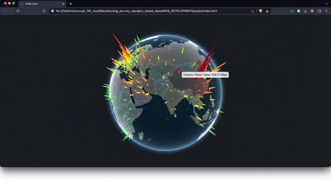
The Core Question You Are Answering
“How do you use InstancedMesh to efficiently render hundreds of data-driven 3D objects, enable per-instance interactivity through raycasting, and smoothly animate camera transitions between different visualization layouts?”
This question matters because 3D data visualization is a growing field with real commercial value. Dashboards, analytics tools, and presentation platforms increasingly use 3D to make data more engaging and explorable. The techniques here – InstancedMesh for performance, raycasting for interactivity, camera animation for navigation, and HTML overlay for UI – are the building blocks of any interactive 3D data application.
Concepts You Must Understand First
- InstancedMesh and Per-Instance Data
- How does InstancedMesh render hundreds of identical geometries in a single draw call? How do you set per-instance position, scale, and color using
setMatrixAt()andsetColorAt()? - Reference: Three.js docs - InstancedMesh
- How does InstancedMesh render hundreds of identical geometries in a single draw call? How do you set per-instance position, scale, and color using
- Raycasting on InstancedMesh
- How does
intersectObjects()work with InstancedMesh? What does theinstanceIdproperty of the intersection tell you? - How does performance compare to raycasting against N individual meshes? (InstancedMesh raycasting tests against each instance’s bounding box derived from its transformation matrix, which can be expensive for thousands of instances.)
- Reference: Three.js docs - Raycaster, InstancedMesh
- How does
- Spherical to Cartesian Coordinate Conversion
- How do you convert latitude/longitude (degrees) to XYZ positions on a sphere?
- What is the difference between geographic coordinates (lat/lon) and Three.js coordinates (X right, Y up, Z toward camera)?
- How do you handle the fact that latitude 0 is the equator (Y=0 on the sphere) but longitude 0 is the prime meridian (X/Z depend on orientation)?
- Book Reference: “Math for Programmers” by Paul Orland - Ch. 3 (3D vectors, coordinate systems)
- Camera Animation with Lerp and Slerp
- What is linear interpolation (lerp) for positions and spherical linear interpolation (slerp) for rotations? How do you animate between two camera states smoothly?
- What easing function produces the most natural camera movement? (Smoothstep or ease-out cubic gives a natural deceleration at the end.)
- How do you prevent the camera from intersecting the globe during the animation? (Ensure the interpolated path stays above the globe surface.)
- Book Reference: “Math for Programmers” by Paul Orland - Ch. 4-5 (Transforms)
- HTML/CSS Overlay Positioning
- How do you project a 3D world position to 2D screen coordinates using
vector.project(camera)and then position an HTML element at those coordinates? - The projection formula: after
vec.project(camera), convert NDC to pixels:x = (vec.x * 0.5 + 0.5) * canvasWidth,y = (-vec.y * 0.5 + 0.5) * canvasHeight. Note: Y is inverted because screen Y increases downward but NDC Y increases upward. - How do you handle bars on the back of the globe (behind the camera)? Check
vec.z > 1after projection – if true, the point is behind the camera and the tooltip should be hidden. - Reference: Three.js docs - Vector3.project
- How do you project a 3D world position to 2D screen coordinates using
Questions to Guide Your Design
- Data Format and Loading
- What data format do you use? A JSON array of
{ country, lat, lon, value }objects? - Do you hardcode the data or load it from an external file/API?
- What data format do you use? A JSON array of
- Bar Orientation on a Sphere
- Each bar must point radially outward from the globe center. How do you compute the rotation matrix for each instance so its local Y axis aligns with the radial direction at its latitude/longitude?
- Can you use
Object3D.lookAt()to compute the matrix, then transfer it to the InstancedMesh?
- Tooltip Positioning
- How do you project the 3D position of the hovered bar’s top to 2D screen coordinates for tooltip placement?
- How do you handle tooltips for bars on the back of the globe (not visible)?
- View Transition Animation
- When switching from globe to bar chart, how do you animate each bar from its spherical position to its bar chart position?
- Do you use a per-instance animation (each bar moves independently) or a global camera transition?
- Performance with 100+ Instances
- InstancedMesh can handle thousands of instances. At 100 countries, is there any performance concern?
- How does raycasting performance scale with instance count?
- Accessibility
- How do you make the visualization accessible to users who cannot interact with 3D? (Data table fallback, keyboard navigation, screen reader labels)
Thinking Exercise
Exercise: Map Country Data to 3D Bars
Take five countries and trace the data-to-visual pipeline:
| Country | Lat | Lon | Population (M) |
|---|---|---|---|
| Brazil | -14.2 | -51.9 | 216 |
| Japan | 36.2 | 138.3 | 125 |
| Nigeria | 9.1 | 8.7 | 224 |
| Germany | 51.2 | 10.4 | 84 |
| Australia | -25.3 | 133.8 | 26 |
For each country:
- Convert lat/lon to radians:
latRad = lat * PI / 180,lonRad = lon * PI / 180 - Convert to Cartesian:
x = R * cos(latRad) * cos(lonRad),y = R * sin(latRad),z = R * cos(latRad) * sin(lonRad)(where R = globe radius, e.g., 5) - Compute bar height: normalize population to a range (e.g., 0.5 to 3.0 units)
- Compute the rotation that aligns the bar’s Y axis with the radial direction at that point
- Build a 4x4 transformation matrix combining position, rotation, and scale
- Set it on the InstancedMesh:
instancedMesh.setMatrixAt(i, matrix)
For each country, show the intermediate computation:
Brazil: lat=-14.2, lon=-51.9, pop=216M
latRad = -14.2 * PI / 180 = -0.2478 rad
lonRad = -51.9 * PI / 180 = -0.9058 rad
x = 5 * cos(-0.2478) * cos(-0.9058) = 5 * 0.9687 * 0.6225 = 3.015
y = 5 * sin(-0.2478) = 5 * -0.2453 = -1.227
z = 5 * cos(-0.2478) * sin(-0.9058) = 5 * 0.9687 * (-0.7826) = -3.791
Position: (3.015, -1.227, -3.791)
Bar height: 216/224 * 2.5 + 0.5 = 2.91 (normalized to 0.5-3.0 range)
Japan: lat=36.2, lon=138.3, pop=125M
latRad = 36.2 * PI / 180 = 0.6318 rad
lonRad = 138.3 * PI / 180 = 2.4136 rad
x = 5 * cos(0.6318) * cos(2.4136) = 5 * 0.8090 * (-0.7431) = -3.006
y = 5 * sin(0.6318) = 5 * 0.5901 = 2.951
z = 5 * cos(0.6318) * sin(2.4136) = 5 * 0.8090 * 0.6691 = 2.707
Position: (-3.006, 2.951, 2.707)
Bar height: 125/224 * 2.5 + 0.5 = 1.895
Questions to answer:
- Why does Australia’s Y coordinate have a negative sign? (Australia is in the Southern Hemisphere with negative latitude. sin(negative angle) produces a negative Y value, placing it below the globe’s equator.)
- If two countries are very close on the globe (e.g., Netherlands and Belgium), how do you prevent their bars from overlapping? (You have several options: use thinner bar geometry, offset overlapping bars slightly in the tangent plane, merge nearby countries into regions, or use a minimum angular distance filter. For this project, thin bars with small radius work for most cases.)
- How do you handle the bar chart layout: what determines the X position of each bar? (Sort countries by value (descending). Space bars evenly along the X axis with fixed gap. The leftmost bar is the highest value. Use the sorted index to compute X:
x = index * (barWidth + gap) - totalWidth/2. Y height remains the data value. Z is 0 for all bars in flat view.) - How do you compute the rotation matrix to orient a bar radially outward from a sphere? (The bar’s local Y axis must point along the radial direction. The radial direction at point P on the sphere is simply the normalized position vector:
radialDir = normalize(P). Usequaternion.setFromUnitVectors(new Vector3(0,1,0), radialDir)to rotate the bar’s Y axis to align with the radial direction.)
The Interview Questions They Will Ask
- “What is InstancedMesh in Three.js and why would you use it for data visualization instead of creating individual Mesh objects?”
- “How do you convert geographic latitude/longitude coordinates to 3D positions on a sphere?”
- “How does raycasting work with InstancedMesh? How do you identify which specific instance was clicked?”
- “Describe how you would animate the camera from one position to another smoothly. What interpolation methods would you use?”
- “How do you position an HTML tooltip element to follow a 3D object as the scene rotates? What is the projection step?”
- “What are the tradeoffs between rendering data as 3D bars on a globe versus a 2D chart? When is 3D visualization actually more useful?”
Hints in Layers
Hint 1: Start With a Globe and Static Bars Create a SphereGeometry globe with a world map texture. Hardcode five countries with their lat/lon. Convert to XYZ positions and create five individual BoxMesh objects at those positions, oriented radially outward. Verify the bars point away from the globe surface correctly before converting to InstancedMesh.
Hint 2: Convert to InstancedMesh
Replace the five individual meshes with a single InstancedMesh. Create a dummy Object3D to help compute transformation matrices: set its position to the bar’s XYZ, use lookAt(0, 0, 0) to orient it toward the center, rotate it by PI/2 on X to flip the Y axis outward, set the scale’s Y component to the bar height. Copy the matrix to the InstancedMesh with setMatrixAt().
Hint 3: Add Hover Raycasting
In the mousemove handler, set up the Raycaster from the camera through the mouse position. Intersect against the InstancedMesh. The intersection result includes instanceId, which tells you which data entry was hovered. Use this index to look up country name and value from your data array. Position a tooltip div at the mouse coordinates.
Hint 4: Animate Camera on Click
Store the camera’s current position and target position (above the clicked country). In the animation loop, if a camera animation is active, lerp the camera position from start to end using a progress value (0 to 1) that increases by delta / animationDuration each frame. Apply an easing function (e.g., t * t * (3 - 2 * t) for smoothstep) to make the movement decelerate at the end.
Books That Will Help
| Topic | Book | Chapter |
|---|---|---|
| 3D coordinate systems | “Math for Programmers” by Paul Orland | Ch. 3 (Ascending to 3D) |
| Vector math for positions | “Math for Programmers” by Paul Orland | Ch. 2 (Drawing with 2D vectors) |
| Transformations and matrices | “Math for Programmers” by Paul Orland | Ch. 4-5 (Transforms, Matrices) |
| Perspective projection | “Computer Graphics from Scratch” by Gabriel Gambetta | Ch. 9 (Perspective Projection) |
Common Pitfalls and Debugging
Problem 1: “Bars point in random directions instead of radially outward from the globe”
- Why: The transformation matrix does not correctly orient the bar’s local Y axis along the radial direction. Using
lookAt(0,0,0)makes the bar’s Z axis point at the center, not its Y axis. - Fix: After using
lookAt(0, 0, 0)on the dummy Object3D, apply an additional rotation ofPI/2on the X axis (or the appropriate axis) to flip the orientation so the Y axis points outward. Alternatively, usequaternion.setFromUnitVectors(new Vector3(0,1,0), radialDirection)to directly align Y to the radial direction. - Quick test: Set all bars to the same height and color. Visually verify they all protrude perpendicular to the globe surface.
Problem 2: “Raycasting on InstancedMesh returns no intersections”
- Why: The InstancedMesh’s bounding volumes may not be updated after setting instance matrices. Or you are calling
intersectObjectswith the wrong reference. - Fix: After setting all instance matrices, call
instancedMesh.instanceMatrix.needsUpdate = trueandinstancedMesh.computeBoundingBox()/instancedMesh.computeBoundingSphere(). Pass the InstancedMesh inside an array tointersectObjects. - Quick test: Add a regular Mesh at the same position as one bar. Does raycasting detect the regular mesh? If yes, the issue is with InstancedMesh setup.
Problem 3: “Tooltip appears in the wrong position or does not follow the bar”
- Why: The 3D-to-2D projection formula is off.
Vector3.project(camera)returns NDC coordinates (-1 to 1), which must be converted to pixel coordinates. - Fix: After
vector.project(camera), convert to pixels:x = (vector.x * 0.5 + 0.5) * canvas.width,y = (-vector.y * 0.5 + 0.5) * canvas.height. Note the Y inversion. Also check if the bar is behind the camera (vector.z > 1 means behind) and hide the tooltip in that case. - Quick test: Position the tooltip at screen center (0, 0 NDC) and verify it appears at the center of the viewport.
Problem 4: “Camera animation jerks or overshoots the target”
- Why: Using raw lerp without proper easing or with a progress value that exceeds 1.0. Or calling
camera.lookAt()during the lerp, which conflicts with the interpolated rotation. - Fix: Clamp the progress value to
Math.min(progress, 1.0). Apply a smoothstep easing function for natural deceleration. Do not callcamera.lookAt()during the animation; instead, interpolate the camera’s quaternion separately usingquaternion.slerp(target, t). - Quick test: Log the progress value each frame. Verify it smoothly increases from 0 to 1 and stops exactly at 1.
Definition of Done
- A textured globe renders and rotates slowly
- Data bars (minimum 50 countries) are positioned at correct geographic locations using InstancedMesh
- Bar heights represent real data values (population, GDP, or similar)
- Bar colors encode data magnitude (blue/yellow/red gradient)
- Hovering over a bar highlights it and shows an HTML tooltip with country name and value
- Clicking a bar smoothly animates the camera to zoom into that region
- A “Back” button returns the camera to the default globe view
- A toggle switches between globe view and flat bar chart view with animated transition
- The visualization handles window resizing correctly
- Performance is smooth (60fps) with 100 InstancedMesh instances
Project 13: Responsive 3D Portfolio Website
| Project 14: Build a Mini Game Engine Architecture | Mini Game Engine Architecture for Three.js, Performance Optimization, Rendering Pipeline | | Project 15: Build a Third-Person Character Controller with Animation Blending | Advanced Animation System and Character Controllers, Performance Optimization, Rendering Pipeline | | Project 16: Build a Multiplayer Web Arena Game | Real-Time Multiplayer Architecture on the Web, Performance Optimization, Rendering Pipeline | | Project 17: Build a Destructible Physics Sandbox | Advanced Physics and Collision Systems, Performance Optimization, Rendering Pipeline | | Project 18: Generate an Infinite Terrain World | Procedural World Generation at Scale, Performance Optimization, Rendering Pipeline | | Project 19: Build a Stylized Shader Lab (Toon, Water, Fire) | Custom Shader Mastery and Stylized Rendering, Performance Optimization, Rendering Pipeline | | Project 20: Build a Post-Processing Engine without EffectComposer | Post-Processing Pipeline Engineering, Performance Optimization, Rendering Pipeline | | Project 21: Optimize a Heavy Scene to 60 FPS on Mobile | Performance Engineering for Mobile 60 FPS, Performance Optimization, Rendering Pipeline | | Project 22: Build a WebXR VR Room with Hand and AR Interaction | WebXR VR and AR Systems, Performance Optimization, Rendering Pipeline | | Project 23: Build a Full Asset Pipeline from Blender to Three.js | Production Asset Pipeline: Blender to Runtime, Performance Optimization, Rendering Pipeline | | Project 24: Implement a Dynamic Day/Night Lighting System | Advanced Lighting and Time-of-Day Systems, Performance Optimization, Rendering Pipeline | | Project 25: Build an In-World UI + HUD Integration System | 3D UI Architecture and Interaction Design, Performance Optimization, Rendering Pipeline | | Project 26: Create a Dynamically Streamed 3D City | Large-Scale World Streaming and Memory Control, Performance Optimization, Rendering Pipeline | | Project 27: Build NPC Navigation with Navmesh, A*, and Behavior Trees | AI and Navigation Systems for NPC Behavior, Performance Optimization, Rendering Pipeline | | Project 28: Recreate a Simplified PBR Rendering Pipeline | Engine-Level Rendering: BRDF and Tone Mapping, Performance Optimization, Rendering Pipeline |
- File: P13-responsive-3d-portfolio.md
- Main Programming Language: JavaScript
- Alternative Programming Languages: TypeScript, Svelte (with threlte)
- Coolness Level: 4 - Impressive (People lean in when they see it)
- Business Potential: 2 - Niche (Useful in specific domains)
- Difficulty: Advanced
- Knowledge Area: Integration / Performance / Production
- Software or Tool: Three.js, GLTFLoader, GSAP (or manual animation), lil-gui (dev mode only)
- Main Book: “Computer Graphics from Scratch” by Gabriel Gambetta - Ch. 9-10 (Perspective Projection, Scene Description)
What you will build: A professional portfolio landing page where 3D elements respond to scrolling. The hero section features a floating 3D object (robot, astronaut, or geometric sculpture) that rotates based on scroll position. As the user scrolls, the camera flies through a 3D scene. Project showcase cards tilt in 3D on hover (parallax effect). The site works on mobile with graceful fallbacks. Performance stays at 60fps on modern devices.
Why it teaches Three.js: This project is the final integration challenge. It combines everything you have learned – GLTF loading, animation, camera movement, post-processing, responsive design, and performance optimization – into a real, deployable product. Unlike isolated demos, a portfolio website must work across devices, load fast, handle edge cases, and feel polished. This is where you learn to ship Three.js in production.
Core challenges you will face:
- Scroll-Driven 3D Animation -> Maps to concept: Animation / DOM Integration
- Responsive 3D Across Devices -> Maps to concept: Camera Systems / Performance
- GLTF Model Loading with Performance Budget -> Maps to concept: Asset Loading / Optimization
- CSS/3D Integration -> Maps to concept: DOM and Canvas Layering
- Production Performance Optimization -> Maps to concept: Performance Optimization
Real World Outcome
When you open the browser on a desktop, the page loads in under 3 seconds. The landing page is a single long-scrolling page with multiple sections, blending traditional HTML/CSS content with Three.js 3D elements.
Section 1: Hero (100vh)
The hero section fills the entire viewport. The Three.js canvas is positioned behind the HTML content (using CSS position: fixed or absolute with z-index layering). The background is a dark gradient (deep blue to black).
A 3D object floats at the center of the hero: a stylized robot, astronaut, geometric sculpture, or abstract mesh loaded from a GLTF file. The object has a MeshStandardMaterial with moderate metalness (0.3) and low roughness (0.2), catching environmental reflections from a subtle HDRI environment map. A soft UnrealBloomPass makes the object’s bright edges glow subtly.
The 3D object gently bobs up and down (sine wave on Y position) and rotates slowly on the Y axis. As you begin scrolling down, the object’s rotation accelerates, and it tilts backward as if being pushed by the scroll. The scroll position maps directly to rotation: at scroll 0%, the object faces forward; at 100% of the hero section, it has rotated 180 degrees and tilted back 30 degrees.
Overlaid on top of the canvas is the HTML content: your name in large type, a one-line tagline, and a “See My Work” call-to-action button. These elements use CSS with pointer-events: auto so they are clickable above the canvas.
Section 2: About (100vh)
As you scroll into the About section, the 3D camera begins a fly-through: it moves from the hero position forward and slightly downward, passing through a tunnel of floating geometric shapes. Approximately 30-50 geometric primitives (torus, icosahedron, octahedron, dodecahedron, torus knot) are scattered in 3D space along the camera’s path, positioned at various distances from the center axis.
The shapes have low-poly wireframe materials in muted accent colors (soft purple, teal, coral) with MeshBasicMaterial and wireframe: true. Each shape rotates slowly on its own axis (random rotation speeds set at initialization), creating gentle movement independent of scrolling.
The scroll position drives the camera’s Z position linearly. At 0% into this section, the camera is at the tunnel entrance. At 100%, it exits the other end. The total camera travel distance is approximately 40 units. The geometric shapes parallax at different speeds depending on their distance from the camera path center:
- Shapes within 3 units of center: move past quickly (1:1 with camera Z)
- Shapes 3-8 units away: move at 0.6x camera speed
- Shapes beyond 8 units: move at 0.3x camera speed (background layer)
This depth-based parallax creates a convincing sense of three-dimensional space as you scroll. Shapes near the camera whoosh past while distant shapes drift slowly.
An HTML text block with your bio sits centered in the viewport using CSS position: sticky, with the 3D tunnel visible behind and around it. The text has a semi-transparent dark background (rgba(0,0,0,0.7)) so it remains readable against the moving 3D shapes.
Section 3: Projects (200vh+)
The Projects section displays 4-6 project cards in a grid layout (2 columns on desktop, 1 on mobile). Each card is a standard HTML element, but it has a CSS 3D transform applied on hover: as you move the mouse across the card, it tilts in the direction of the cursor (using transform: perspective(1000px) rotateX(Xdeg) rotateY(Ydeg)). This is pure CSS/JS parallax tilt – not rendered in the Three.js canvas.
Each card has a small 3D icon or thumbnail rendered in a separate small Three.js canvas (or a pre-rendered animated GIF/WebP). The icon is a simple rotating 3D shape related to the project topic.
As you scroll the projects section into view, cards animate in from below with a staggered fade-in (each card appears 100ms after the previous one), using either GSAP ScrollTrigger or Intersection Observer API.
Section 4: Contact (50vh)
The contact section has a simple form (name, email, message) with the 3D canvas showing a subtle particle field in the background – slowly drifting white dots that react slightly to mouse position (push away from the cursor). A footer with social links sits at the bottom.
Responsive Behavior:
On tablet (768px-1024px):
- The hero 3D object scales down slightly (camera FOV increases or object scales to 0.7).
- The tunnel shapes in Section 2 reduce from 40 to 15 (fewer floating objects).
- Post-processing bloom is disabled (saves one full-screen pass).
- Project cards switch to single column.
- Shadows are disabled.
- Pixel ratio is capped at 1.5.
On mobile (< 768px):
- The 3D hero object is replaced with a static or CSS-animated fallback:
- Option A: A subtle gradient animation using CSS
@keyframes(zero GPU cost). - Option B: A pre-rendered short video loop (MP4/WebM, < 500KB) of the 3D object captured from the desktop version.
- Option C: A single high-quality screenshot of the 3D scene as a static background image with a CSS parallax effect.
- Option A: A subtle gradient animation using CSS
- The scroll-driven tunnel in Section 2 is disabled entirely – shows a simple gradient background with CSS-animated geometric shapes (divs with
border-radiusandtransform). - Project cards use simplified tilt (or no tilt).
- The contact particle field uses fewer particles (500 instead of 2000) or is replaced with a CSS dot pattern.
- Three.js is not loaded at all on mobile (tree-shaken out or lazy-loaded only on desktop). This saves ~150KB of JavaScript and all GPU overhead.
This mobile fallback is critical: many mobile devices struggle with complex WebGL, and the user experience must remain smooth. The detection uses a combination of signals:
window.innerWidth < 768for screen sizenavigator.maxTouchPoints > 0for touch capabilitynavigator.hardwareConcurrency < 4as a CPU capability proxy- WebGL context test: attempt to create a WebGL2 context and check
renderer.capabilities
The detection runs once at page load and sets a global deviceTier variable: “desktop”, “tablet”, or “mobile”. Each section checks this variable to determine what to render.
Performance Budget:
| Metric | Desktop Target | Mobile Target | How to Measure |
|---|---|---|---|
| First Contentful Paint | < 1.5s | < 2.0s | Chrome Lighthouse |
| Largest Contentful Paint | < 3.0s | < 4.0s | Chrome Lighthouse |
| Total JavaScript bundle | < 500KB gzip | < 200KB gzip | Webpack Bundle Analyzer |
| GLTF model | < 2MB (Draco) | Not loaded | Network tab |
| Textures | < 1MB total | < 200KB | renderer.info.memory |
| Draw calls per frame | < 50 | < 20 | renderer.info.render.calls |
| Triangles per frame | < 100K | < 20K | renderer.info.render.triangles |
| Frame rate | 60fps | 30fps+ (if 3D active) | stats.js |
| Total page weight | < 5MB | < 2MB | Network tab |
| Time to Interactive | < 3.5s | < 5.0s | Chrome Lighthouse |
A hidden stats.js panel (toggled with a keyboard shortcut like Shift+S) shows FPS during development. In production, stats.js should not be loaded at all (removed from the production build or behind a debug flag).
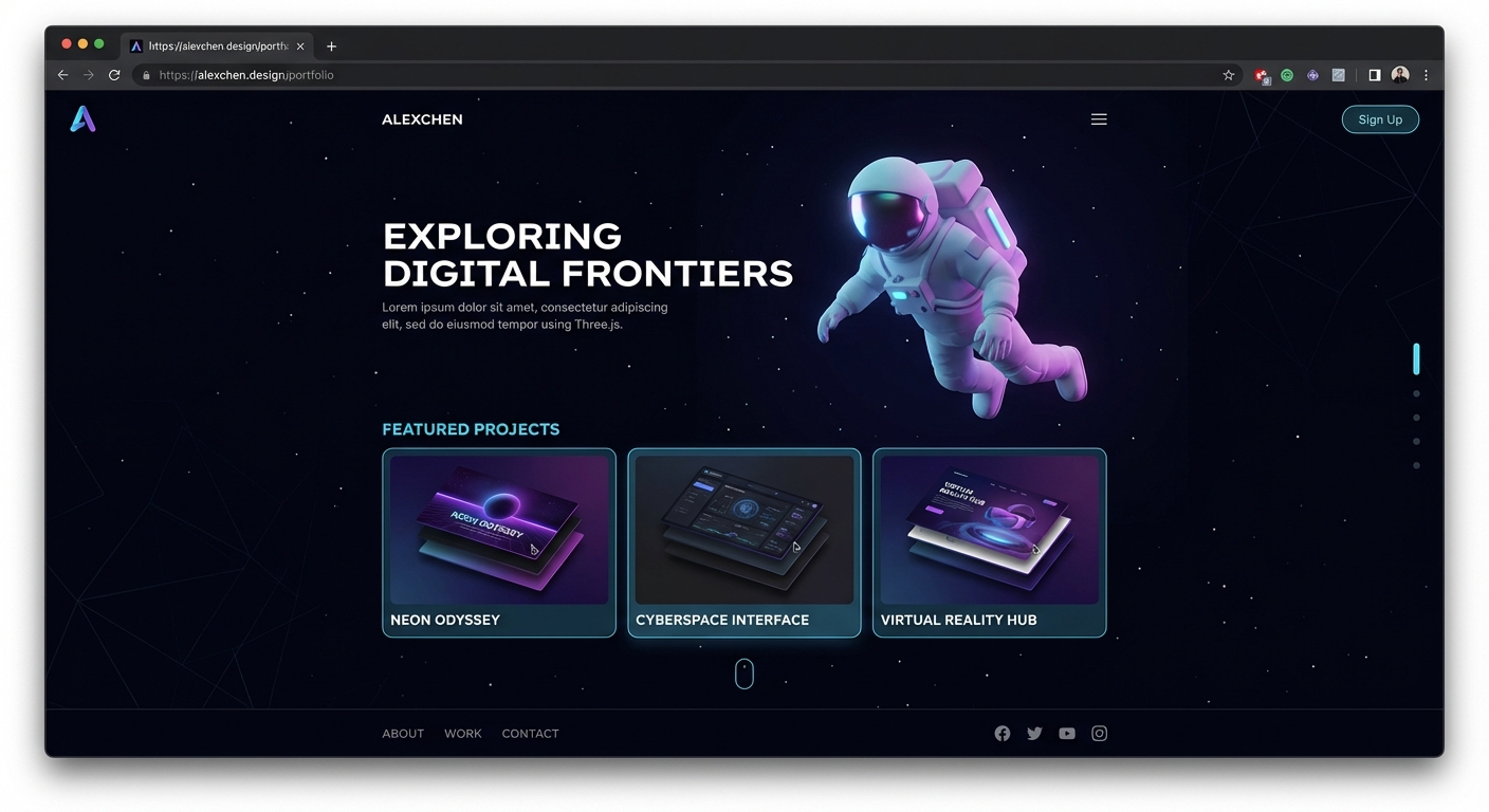
The Core Question You Are Answering
“How do you integrate Three.js into a production website with scroll-driven animation, responsive design, and strict performance budgets – and how do you gracefully degrade on low-powered devices?”
This question matters because deploying Three.js in production is fundamentally different from building demos. In production, you must handle: page load performance (lazy loading, asset compression), responsive design (different device capabilities), scroll synchronization (smooth mapping of scroll position to 3D state), accessibility (the page must work without 3D), and performance budgets (real users on real devices). This project teaches you to think like a production engineer, not just a creative coder.
Concepts You Must Understand First
- Scroll-to-Animation Mapping
- How do you convert
window.scrollYor an Intersection Observer ratio into a normalized 0-1 value that drives 3D transformations? - Reference: GSAP ScrollTrigger documentation, MDN Intersection Observer API
- How do you convert
- CSS and Canvas Layering
- How do you position a Three.js canvas behind HTML content using CSS z-index, and how do you handle pointer events so HTML elements remain clickable?
- Reference: MDN - CSS Stacking Context, pointer-events
- Responsive Breakpoint Detection
- How do you detect device capability and switch between full 3D (desktop), reduced 3D (tablet), and no 3D (mobile)?
- Reference: MDN - matchMedia, Window.innerWidth
- GLTF Loading with Loading Manager
- How do you show a loading progress bar while GLTF and texture assets download, and how do you handle loading failures gracefully?
- Reference: Three.js docs - LoadingManager
- Performance Budgeting
- How do you set pixel ratio caps (
Math.min(devicePixelRatio, 2)), limit draw calls, compress assets, and lazy-load 3D content? - Reference: Three.js docs - WebGLRenderer, Discover Three.js - Performance chapter
- How do you set pixel ratio caps (
- Parallax Tilt Effect (CSS)
- How do you map mouse position on a card to rotateX and rotateY CSS transforms with perspective?
- Reference: CSS Tricks - Tilt Hover Effects
Questions to Guide Your Design
- Canvas Strategy
- Do you use one full-screen fixed canvas for the entire page, or multiple smaller canvases for each section?
- A single canvas is simpler but renders even when not visible. Multiple canvases allow independent lifecycle management but add complexity.
- Scroll Synchronization
- How do you prevent scroll jank? (Hint: read scroll position in requestAnimationFrame, not in the scroll event handler.)
- How do you handle the case where the user scrolls very quickly through sections?
- Asset Loading Strategy
- Do you load all 3D assets at page load, or lazy-load them as sections come into view?
- What does the user see while assets are loading?
- Mobile Detection and Fallback
- Do you detect mobile by screen width, touch capability, or GPU capability? Which is most reliable?
- What specific Three.js features do you disable on mobile (post-processing, shadows, particle count)?
- Deployment
- How do you bundle Three.js for production? (Tree-shaking with Vite or Webpack, importing only used modules:
import { Scene, PerspectiveCamera } from 'three'instead ofimport * as THREE from 'three') - How do you ensure the GLTF model loads from the correct path in production? (Use relative paths from the public directory, or configure the base URL in your bundler)
- How do you implement code splitting so Three.js only loads on desktop? (Dynamic
import()behind a device-tier check:if (deviceTier === 'desktop') { const THREE = await import('three') })
- How do you bundle Three.js for production? (Tree-shaking with Vite or Webpack, importing only used modules:
- Accessibility
- Is the page usable with JavaScript disabled? (Static HTML fallback with basic CSS styling should render all text content, navigation, and project cards)
- Do screen readers announce anything meaningful for the 3D sections? (Add
aria-hidden="true"to the canvas element. Provide equivalent text descriptions in hidden elements withsr-onlyclass) - Can keyboard-only users navigate all interactive elements? (Tab order should reach all links, buttons, and form fields. The 3D canvas is decorative and should be skipped in tab order)
- Does the site respect
prefers-reduced-motion? (Checkwindow.matchMedia('(prefers-reduced-motion: reduce)')and disable all animations if true, including 3D rotation and scroll-driven effects)
Thinking Exercise
Exercise: Design the Scroll-to-3D Mapping
Map the entire page scroll to 3D state changes:
Page height: 450vh total (100 + 100 + 200 + 50)

Scroll 0vh - 100vh (Hero Section):
  - 3D object Y rotation: 0deg -> 180deg (linear)
  - 3D object Y position: 0 -> -0.5 (bob stops, sinks)
  - 3D object X tilt: 0deg -> 30deg (leans back)
  - HTML title opacity: 1.0 -> 0.0 (fades out)

Scroll 100vh - 200vh (About Section):
  - Camera Z position: 0 -> -20 (fly through tunnel)
  - Floating shapes parallax: each shape.z += scrollDelta * (1.0 / distanceFromCenter)
  - HTML about text opacity: 0 -> 1 -> 0 (fade in then out)

Scroll 200vh - 400vh (Projects Section):
  - No 3D camera movement (static)
  - Cards animate in via Intersection Observer
  - Tilt on hover (mouse-driven, not scroll-driven)

Scroll 400vh - 450vh (Contact Section):
  - Background particles drift speed increases slightly
  - Camera Z: static
Questions to answer:
- How do you compute a 0-1 progress value for each section?
sectionStart = section.offsetTop
sectionHeight = section.clientHeight
progress = clamp((scrollY - sectionStart) / sectionHeight, 0, 1)
This gives 0 when the section top aligns with the viewport top, and 1 when the section is fully scrolled past.
-
What happens if the user uses browser smooth scrolling versus instant jumps? (With smooth scrolling, scroll events fire rapidly with small deltas – the animation looks smooth. With instant jumps (anchor links, Page Down), scrollY changes by a large amount in one frame. If you lerp the 3D state, the animation catches up smoothly. If you apply scrollY directly, the 3D state jumps instantly, which can look jarring.)
-
How do you ensure the 3D object’s rotation does not “jump” when scrolling back up? (Map the rotation directly to scroll progress, not to scroll delta.
rotation.y = progress * Math.PIproduces the same rotation at the same scroll position regardless of scroll direction. If you accumulate rotation from scroll deltas, scrolling up then down produces different rotations at the same position.) - What is the total number of 3D state variables controlled by scroll? (In this design: hero object Y rotation, Y position, X tilt = 3 variables. Camera Z position = 1 variable. Floating shape positions = N variables. Total: 4 + N. Each must be computed from the section progress value in every animation frame.)
The Interview Questions They Will Ask
- “How would you integrate a Three.js scene into an existing website without affecting page performance or scroll behavior?”
- “Describe your approach to making a 3D web experience responsive across desktop, tablet, and mobile devices.”
- “What performance optimizations would you apply to ship Three.js in production? Walk me through your performance budget.”
- “How do you synchronize scroll position with 3D animation without causing jank or frame drops?”
- “How would you handle the case where WebGL is not supported or the device is too slow for 3D rendering?”
- “Describe the asset loading strategy for a production Three.js site. How do you minimize time-to-interactive?”
Hints in Layers
Hint 1: Start With Scroll Mapping Forget Three.js initially. Create a plain HTML page with four colored sections (100vh each). Add a scroll event listener that computes a 0-1 progress value for each section. Log the values to the console. Verify that scrolling through Section 1 produces a smooth 0-to-1 ramp while other sections remain at 0 or 1. This scroll math is the foundation of everything.
Hint 2: Add the Canvas Layer
Create a Three.js scene with a simple rotating cube on a fixed canvas (position: fixed; top: 0; left: 0; z-index: -1). In the animation loop, read the stored scroll progress value (captured in the scroll handler) and map it to the cube’s Y rotation: cube.rotation.y = scrollProgress * Math.PI. The cube should rotate as you scroll. HTML content should be visible above the canvas.
Hint 3: Load the GLTF Hero Object Replace the cube with a GLTF model. Add a LoadingManager that shows a CSS loading bar while the model downloads. Once loaded, apply the same scroll-driven rotation. Add the bobbing animation (sine wave on Y) that runs independently of scroll. Add bloom post-processing with low strength (0.3) for subtle glow.
Hint 4: Responsive Fallback
Add a media query check: if (window.innerWidth < 768). If true, skip creating the Three.js scene entirely. Instead, show a CSS-animated gradient background or a pre-rendered video of the 3D scene as a fallback. On tablet (768-1024), create the Three.js scene but disable post-processing and reduce model quality. Test on Chrome DevTools device simulator.
Books That Will Help
| Topic | Book | Chapter |
|---|---|---|
| Perspective and projection | “Computer Graphics from Scratch” by Gabriel Gambetta | Ch. 9 (Perspective Projection) |
| Scene description | “Computer Graphics from Scratch” by Gabriel Gambetta | Ch. 10 (Describing a Scene) |
| 3D coordinates and transforms | “Math for Programmers” by Paul Orland | Ch. 2-5 (Vectors through Matrices) |
| Performance optimization | “Real-Time Rendering” by Akenine-Moller et al. | Ch. 10 (Pipeline Optimization) |
| Shader fundamentals for effects | “The Book of Shaders” by Gonzalez Vivo | Ch. 1-3 (Getting started) |
Common Pitfalls and Debugging
Problem 1: “Scroll-driven animation is jittery and stutters”
- Why: Reading
window.scrollYinside a scroll event listener and immediately updating Three.js creates jank because scroll events fire at unpredictable rates (not synchronized with requestAnimationFrame). Multiple scroll events may fire between renders, or none may fire during a render frame. - Fix: In the scroll event handler, only store the scroll position in a variable. In the requestAnimationFrame loop, read that stored value and apply it to the 3D scene. This decouples scroll reading (which happens at browser event rate) from rendering (which happens at display rate). Optionally smooth the value with lerp:
currentScroll = lerp(currentScroll, targetScroll, 0.1). - Quick test: Log timestamps of scroll events and rAF callbacks. They should fire at different rates. If you see 3D updates happening at scroll event rate, you have jank.
Problem 2: “The page loads slowly because the GLTF model is 15MB”
- Why: Uncompressed GLTF models with high-poly meshes and uncompressed textures are far too large for web delivery.
- Fix: Compress the model geometry with Draco (reduces mesh data by 90%+). Compress textures to WebP or KTX2 (reduces texture size by 75%+). Use gltf-transform CLI:
npx gltf-transform optimize input.glb output.glb --compress draco --texture-compress webp. Target < 2MB total for the hero model. - Quick test: Open Chrome DevTools Network tab. Filter by the model URL. Check the transfer size. Anything over 2MB will cause noticeable loading delays on 3G connections.
Problem 3: “The site works on desktop but crashes or freezes on mobile”
- Why: Mobile GPUs have significantly less processing power. Post-processing, high-poly models, and high pixel ratios (some phones have devicePixelRatio of 3) multiply the GPU workload beyond mobile capability.
- Fix: Cap pixel ratio with
renderer.setPixelRatio(Math.min(window.devicePixelRatio, 2)). Disable post-processing on mobile. Reduce model polygon count or use a lower-LOD model. Disable shadows. Reduce particle count. Or disable Three.js entirely on mobile and use a CSS/video fallback. - Quick test: Open Chrome DevTools, enable device simulation (e.g., iPhone 12), set CPU throttling to 4x slowdown, and GPU throttling. If the FPS drops below 15, mobile users will have a bad experience.
Problem 4: “HTML content is not clickable – clicks go to the canvas instead”
- Why: The Three.js canvas is positioned on top of the HTML content (or at the same z-index), capturing all pointer events.
- Fix: Set the canvas to
pointer-events: nonein CSS so clicks pass through it to the HTML below. If you need Three.js to also receive mouse events (for hover effects), selectively enable them: setpointer-events: noneon the canvas but listen for mouse events ondocumentinstead, or use a transparent overlay div for 3D interactivity. - Quick test: Try clicking the CTA button in the hero section. If nothing happens, the canvas is capturing the event.
Definition of Done
- A single-page portfolio site with at least 3 sections (Hero, About/Projects, Contact)
- Hero section features a GLTF 3D object that responds to scroll position (rotation, tilt)
- The 3D object bobs gently with an idle animation independent of scroll
- Camera or objects animate based on scroll position in at least one section
- Project cards have a hover tilt effect (CSS 3D transforms)
- The site is responsive: full 3D on desktop, reduced or replaced on mobile
- Page loads in under 3 seconds on a fast connection (GLTF < 2MB, compressed)
- FPS stays at 60 on modern desktop hardware
- HTML content is clickable above the canvas (proper z-index and pointer-events)
- A loading state is shown while 3D assets download
renderer.setPixelRatiois capped at 2- The site degrades gracefully if WebGL is not available (basic HTML/CSS still works)
- The site respects
prefers-reduced-motionmedia query (disables animations when set) - All text content is readable and navigable without JavaScript enabled
- The GLTF model is Draco-compressed and under 2MB transfer size
Project 14: Build a Mini Game Engine Architecture
- File: P14-mini-game-engine-architecture.md
- Main Programming Language: TypeScript
- Alternative Programming Languages: JavaScript, Rust (WASM), C# (Unity prototype parity)
- Coolness Level: 5 - Legendary
- Business Potential: 4 - Strong product fit
- Difficulty: Expert
- Knowledge Area: Engine Architecture
- Software or Tool: TypeScript + Three.js
- Main Book: “Game Engine Architecture” by Jason Gregory - runtime architecture chapters
What you will build: A production-style module centered on Mini Game Engine Architecture for Three.js with observable runtime output and measurable correctness signals.
Why it teaches Three.js: It forces you to treat Three.js as a systems runtime, not just a rendering library, by implementing SceneLoader, SceneStack, ECS, game loop abstraction, event bus, dependency injection, and asset cache lifecycles.
Core challenges you will face:
- Boundary design under pressure -> You must keep modules isolated while features grow.
- Runtime correctness verification -> You need explicit invariants and failure tests.
- Performance and operability tradeoffs -> Every abstraction choice affects frame time and memory.
Real World Outcome
When you open the project, you see a functional scenario proving the concept end-to-end, not a toy placeholder. The UI includes a diagnostics panel with frame time, subsystem timings, memory usage, and critical state transitions. Interactions are observable: toggling a subsystem shows measurable impact, failure injection demonstrates recovery behavior, and logs annotate the exact phase where work happened. The project includes a repeatable walkthrough document so a reviewer can run the same sequence and confirm identical outcomes. By the end, you can demonstrate stable behavior under normal load, controlled degradation under stress, and a clear explanation of why the architecture holds.
Observable session transcript (example):
action: boot project result: all subsystem health checks green action: run stress preset result: frame time rises from 11.4ms to 15.8ms, no dropped simulation ticks action: enable debug overlays result: timing histogram and queue depth visible in HUD action: trigger recovery test result: degraded subsystem is isolated and recovers without full restart
The Core Question You Are Answering
“How do you structure Three.js like a maintainable engine instead of a collection of ad-hoc scripts?”
This matters because teams fail less from missing features and more from systems that cannot be reasoned about under change. This project trains you to design for predictability, instrumentation, and controlled growth.
Concepts You Must Understand First
- Deterministic Update Order
- Which systems run first, and what state do they own?
- Book Reference: “Game Engine Architecture” by Jason Gregory - runtime architecture chapters
- Resource Lifecycle Management
- When is data loaded, retained, and evicted?
- Book Reference: “Game Engine Architecture” by Jason Gregory - resource chapters
- Event and Message Boundaries
- Which events are domain events versus UI-only events?
- Book Reference: “Game Programming Patterns” by Robert Nystrom - event queue chapter
- Profiling and Telemetry
- Which metrics prove correctness and performance?
- Book Reference: “Real-Time Rendering” by Akenine-Moller - optimization chapters
Questions to Guide Your Design
- Which state is authoritative, and which state is a derived view?
- What is your fixed-step versus variable-step policy?
- How will you prove subsystem isolation during a failure test?
- What are your frame-time and memory budgets for this project?
- How will you detect regression automatically after adding a new feature?
Thinking Exercise
Exercise: Failure Budget Tabletop
Create a table with three scenarios: latency spike, memory spike, and event storm. For each scenario, trace the exact subsystem boundary where the issue should be contained, the metric that detects it first, and the expected recovery strategy.
Questions to answer:
- Which invariant breaks first in each scenario?
- Which recovery action is safe during the current frame?
- Which signals prove the system returned to healthy state?
The Interview Questions They Will Ask
- “How did you decide system boundaries in this project?”
- “Which metrics did you track to prove the architecture works?”
- “How do you reproduce and debug a non-deterministic bug in real time systems?”
- “What tradeoffs did you make between abstraction and performance?”
- “How would this design evolve if user count or world size doubled?”
Hints in Layers
Hint 1: Start with contracts, not features Write a one-page runtime contract defining ownership, ordering, and lifecycle before implementation.
Hint 2: Instrument early Add telemetry from day one so regressions are visible while the system is still small.
Hint 3: Add controlled failure injection Introduce toggles that simulate delays or dropped events to validate resilience.
Hint 4: Validate with repeatable scripts Use a deterministic scenario playback to compare metrics before and after each change.
Books That Will Help
| Topic | Book | Chapter |
|---|---|---|
| Runtime design | “Game Engine Architecture” by Jason Gregory - runtime architecture chapters | Relevant architecture chapters |
| Performance diagnostics | “Real-Time Rendering” by Akenine-Moller | Pipeline optimization chapters |
| System boundaries | “Game Programming Patterns” by Robert Nystrom | Update, event queue, state |
Common Pitfalls and Debugging
Problem 1: “Behavior differs between runs”
- Why: Update ordering or hidden mutable state is non-deterministic.
- Fix: Enforce deterministic ordering and isolate mutable ownership.
- Quick test: Replay the same deterministic input stream twice and diff telemetry output.
Problem 2: “Performance fixes break correctness”
- Why: Optimizations bypassed invariant checks.
- Fix: Keep invariants explicit and validate them after each optimization pass.
- Quick test: Run correctness assertions with optimization toggles on and off.
Problem 3: “Memory keeps growing”
- Why: Resource eviction policies are missing or too conservative.
- Fix: Add lifecycle states and eviction thresholds tied to scene scope.
- Quick test: Run a long session, capture memory high-water marks, and verify plateau behavior.
Definition of Done
- Core functionality demonstrates Mini Game Engine Architecture for Three.js in a realistic scenario
- Deterministic replay script produces stable outcomes
- Telemetry panel exposes frame, memory, and subsystem timings
- At least one controlled failure injection path is implemented and documented
- Recovery path succeeds without full application restart
- Performance budget stays within documented limits on reference hardware
- Architecture and invariants are documented in a short design note
Project 15: Build a Third-Person Character Controller with Animation Blending
- File: P15-third-person-character-controller.md
- Main Programming Language: TypeScript
- Alternative Programming Languages: JavaScript, Rust (WASM), C# (Unity prototype parity)
- Coolness Level: 5 - Legendary
- Business Potential: 4 - Strong product fit
- Difficulty: Expert
- Knowledge Area: Animation Systems
- Software or Tool: Three.js + GLTF + input stack
- Main Book: “Game Programming Patterns” by Robert Nystrom - state and update loop patterns
What you will build: A production-style module centered on Advanced Animation System and Character Controllers with observable runtime output and measurable correctness signals.
Why it teaches Three.js: It forces you to treat Three.js as a systems runtime, not just a rendering library, by implementing GLTF animation mixer internals, layered animation graphs, crossfades, locomotion state machines, root motion policy, and camera spring constraints.
Core challenges you will face:
- Boundary design under pressure -> You must keep modules isolated while features grow.
- Runtime correctness verification -> You need explicit invariants and failure tests.
- Performance and operability tradeoffs -> Every abstraction choice affects frame time and memory.
Real World Outcome
When you open the project, you see a functional scenario proving the concept end-to-end, not a toy placeholder. The UI includes a diagnostics panel with frame time, subsystem timings, memory usage, and critical state transitions. Interactions are observable: toggling a subsystem shows measurable impact, failure injection demonstrates recovery behavior, and logs annotate the exact phase where work happened. The project includes a repeatable walkthrough document so a reviewer can run the same sequence and confirm identical outcomes. By the end, you can demonstrate stable behavior under normal load, controlled degradation under stress, and a clear explanation of why the architecture holds.
Observable session transcript (example):
action: boot project result: all subsystem health checks green action: run stress preset result: frame time rises from 11.4ms to 15.8ms, no dropped simulation ticks action: enable debug overlays result: timing histogram and queue depth visible in HUD action: trigger recovery test result: degraded subsystem is isolated and recovers without full restart
The Core Question You Are Answering
“How do you make character movement feel intentional, responsive, and believable under real gameplay input?”
This matters because teams fail less from missing features and more from systems that cannot be reasoned about under change. This project trains you to design for predictability, instrumentation, and controlled growth.
Concepts You Must Understand First
- Deterministic Update Order
- Which systems run first, and what state do they own?
- Book Reference: “Game Programming Patterns” by Robert Nystrom - state and update loop patterns
- Resource Lifecycle Management
- When is data loaded, retained, and evicted?
- Book Reference: “Game Engine Architecture” by Jason Gregory - resource chapters
- Event and Message Boundaries
- Which events are domain events versus UI-only events?
- Book Reference: “Game Programming Patterns” by Robert Nystrom - event queue chapter
- Profiling and Telemetry
- Which metrics prove correctness and performance?
- Book Reference: “Real-Time Rendering” by Akenine-Moller - optimization chapters
Questions to Guide Your Design
- Which state is authoritative, and which state is a derived view?
- What is your fixed-step versus variable-step policy?
- How will you prove subsystem isolation during a failure test?
- What are your frame-time and memory budgets for this project?
- How will you detect regression automatically after adding a new feature?
Thinking Exercise
Exercise: Failure Budget Tabletop
Create a table with three scenarios: latency spike, memory spike, and event storm. For each scenario, trace the exact subsystem boundary where the issue should be contained, the metric that detects it first, and the expected recovery strategy.
Questions to answer:
- Which invariant breaks first in each scenario?
- Which recovery action is safe during the current frame?
- Which signals prove the system returned to healthy state?
The Interview Questions They Will Ask
- “How did you decide system boundaries in this project?”
- “Which metrics did you track to prove the architecture works?”
- “How do you reproduce and debug a non-deterministic bug in real time systems?”
- “What tradeoffs did you make between abstraction and performance?”
- “How would this design evolve if user count or world size doubled?”
Hints in Layers
Hint 1: Start with contracts, not features Write a one-page runtime contract defining ownership, ordering, and lifecycle before implementation.
Hint 2: Instrument early Add telemetry from day one so regressions are visible while the system is still small.
Hint 3: Add controlled failure injection Introduce toggles that simulate delays or dropped events to validate resilience.
Hint 4: Validate with repeatable scripts Use a deterministic scenario playback to compare metrics before and after each change.
Books That Will Help
| Topic | Book | Chapter |
|---|---|---|
| Runtime design | “Game Programming Patterns” by Robert Nystrom - state and update loop patterns | Relevant architecture chapters |
| Performance diagnostics | “Real-Time Rendering” by Akenine-Moller | Pipeline optimization chapters |
| System boundaries | “Game Programming Patterns” by Robert Nystrom | Update, event queue, state |
Common Pitfalls and Debugging
Problem 1: “Behavior differs between runs”
- Why: Update ordering or hidden mutable state is non-deterministic.
- Fix: Enforce deterministic ordering and isolate mutable ownership.
- Quick test: Replay the same deterministic input stream twice and diff telemetry output.
Problem 2: “Performance fixes break correctness”
- Why: Optimizations bypassed invariant checks.
- Fix: Keep invariants explicit and validate them after each optimization pass.
- Quick test: Run correctness assertions with optimization toggles on and off.
Problem 3: “Memory keeps growing”
- Why: Resource eviction policies are missing or too conservative.
- Fix: Add lifecycle states and eviction thresholds tied to scene scope.
- Quick test: Run a long session, capture memory high-water marks, and verify plateau behavior.
Definition of Done
- Core functionality demonstrates Advanced Animation System and Character Controllers in a realistic scenario
- Deterministic replay script produces stable outcomes
- Telemetry panel exposes frame, memory, and subsystem timings
- At least one controlled failure injection path is implemented and documented
- Recovery path succeeds without full application restart
- Performance budget stays within documented limits on reference hardware
- Architecture and invariants are documented in a short design note
Project 16: Build a Multiplayer Web Arena Game
- File: P16-multiplayer-web-arena.md
- Main Programming Language: TypeScript
- Alternative Programming Languages: JavaScript, Rust (WASM), C# (Unity prototype parity)
- Coolness Level: 5 - Legendary
- Business Potential: 5 - High monetization potential
- Difficulty: Expert
- Knowledge Area: Networking
- Software or Tool: Node.js WebSocket server + Three.js client
- Main Book: “Multiplayer Game Programming” by Josh Glazer - replication chapters
What you will build: A production-style module centered on Real-Time Multiplayer Architecture on the Web with observable runtime output and measurable correctness signals.
Why it teaches Three.js: It forces you to treat Three.js as a systems runtime, not just a rendering library, by implementing WebSockets transport, server authority boundaries, deterministic tick simulation, client prediction, interpolation buffers, and lag compensation.
Core challenges you will face:
- Boundary design under pressure -> You must keep modules isolated while features grow.
- Runtime correctness verification -> You need explicit invariants and failure tests.
- Performance and operability tradeoffs -> Every abstraction choice affects frame time and memory.
Real World Outcome
When you open the project, you see a functional scenario proving the concept end-to-end, not a toy placeholder. The UI includes a diagnostics panel with frame time, subsystem timings, memory usage, and critical state transitions. Interactions are observable: toggling a subsystem shows measurable impact, failure injection demonstrates recovery behavior, and logs annotate the exact phase where work happened. The project includes a repeatable walkthrough document so a reviewer can run the same sequence and confirm identical outcomes. By the end, you can demonstrate stable behavior under normal load, controlled degradation under stress, and a clear explanation of why the architecture holds.
Observable session transcript (example):
action: boot project result: all subsystem health checks green action: run stress preset result: frame time rises from 11.4ms to 15.8ms, no dropped simulation ticks action: enable debug overlays result: timing histogram and queue depth visible in HUD action: trigger recovery test result: degraded subsystem is isolated and recovers without full restart
The Core Question You Are Answering
“How do you keep many clients synchronized when network latency and packet jitter are unavoidable?”
This matters because teams fail less from missing features and more from systems that cannot be reasoned about under change. This project trains you to design for predictability, instrumentation, and controlled growth.
Concepts You Must Understand First
- Deterministic Update Order
- Which systems run first, and what state do they own?
- Book Reference: “Multiplayer Game Programming” by Josh Glazer - replication chapters
- Resource Lifecycle Management
- When is data loaded, retained, and evicted?
- Book Reference: “Game Engine Architecture” by Jason Gregory - resource chapters
- Event and Message Boundaries
- Which events are domain events versus UI-only events?
- Book Reference: “Game Programming Patterns” by Robert Nystrom - event queue chapter
- Profiling and Telemetry
- Which metrics prove correctness and performance?
- Book Reference: “Real-Time Rendering” by Akenine-Moller - optimization chapters
Questions to Guide Your Design
- Which state is authoritative, and which state is a derived view?
- What is your fixed-step versus variable-step policy?
- How will you prove subsystem isolation during a failure test?
- What are your frame-time and memory budgets for this project?
- How will you detect regression automatically after adding a new feature?
Thinking Exercise
Exercise: Failure Budget Tabletop
Create a table with three scenarios: latency spike, memory spike, and event storm. For each scenario, trace the exact subsystem boundary where the issue should be contained, the metric that detects it first, and the expected recovery strategy.
Questions to answer:
- Which invariant breaks first in each scenario?
- Which recovery action is safe during the current frame?
- Which signals prove the system returned to healthy state?
The Interview Questions They Will Ask
- “How did you decide system boundaries in this project?”
- “Which metrics did you track to prove the architecture works?”
- “How do you reproduce and debug a non-deterministic bug in real time systems?”
- “What tradeoffs did you make between abstraction and performance?”
- “How would this design evolve if user count or world size doubled?”
Hints in Layers
Hint 1: Start with contracts, not features Write a one-page runtime contract defining ownership, ordering, and lifecycle before implementation.
Hint 2: Instrument early Add telemetry from day one so regressions are visible while the system is still small.
Hint 3: Add controlled failure injection Introduce toggles that simulate delays or dropped events to validate resilience.
Hint 4: Validate with repeatable scripts Use a deterministic scenario playback to compare metrics before and after each change.
Books That Will Help
| Topic | Book | Chapter |
|---|---|---|
| Runtime design | “Multiplayer Game Programming” by Josh Glazer - replication chapters | Relevant architecture chapters |
| Performance diagnostics | “Real-Time Rendering” by Akenine-Moller | Pipeline optimization chapters |
| System boundaries | “Game Programming Patterns” by Robert Nystrom | Update, event queue, state |
Common Pitfalls and Debugging
Problem 1: “Behavior differs between runs”
- Why: Update ordering or hidden mutable state is non-deterministic.
- Fix: Enforce deterministic ordering and isolate mutable ownership.
- Quick test: Replay the same deterministic input stream twice and diff telemetry output.
Problem 2: “Performance fixes break correctness”
- Why: Optimizations bypassed invariant checks.
- Fix: Keep invariants explicit and validate them after each optimization pass.
- Quick test: Run correctness assertions with optimization toggles on and off.
Problem 3: “Memory keeps growing”
- Why: Resource eviction policies are missing or too conservative.
- Fix: Add lifecycle states and eviction thresholds tied to scene scope.
- Quick test: Run a long session, capture memory high-water marks, and verify plateau behavior.
Definition of Done
- Core functionality demonstrates Real-Time Multiplayer Architecture on the Web in a realistic scenario
- Deterministic replay script produces stable outcomes
- Telemetry panel exposes frame, memory, and subsystem timings
- At least one controlled failure injection path is implemented and documented
- Recovery path succeeds without full application restart
- Performance budget stays within documented limits on reference hardware
- Architecture and invariants are documented in a short design note
Project 17: Build a Destructible Physics Sandbox
- File: P17-destructible-physics-sandbox.md
- Main Programming Language: TypeScript
- Alternative Programming Languages: JavaScript, Rust (WASM), C# (Unity prototype parity)
- Coolness Level: 5 - Legendary
- Business Potential: 4 - Strong product fit
- Difficulty: Expert
- Knowledge Area: Physics
- Software or Tool: Rapier or Ammo.js + Three.js
- Main Book: “Game Physics Engine Development” by Ian Millington - constraints and collision chapters
What you will build: A production-style module centered on Advanced Physics and Collision Systems with observable runtime output and measurable correctness signals.
Why it teaches Three.js: It forces you to treat Three.js as a systems runtime, not just a rendering library, by implementing Compound colliders, CCD, constraints, joints, raycast vehicles, fracture event pipelines, and debug overlays.
Core challenges you will face:
- Boundary design under pressure -> You must keep modules isolated while features grow.
- Runtime correctness verification -> You need explicit invariants and failure tests.
- Performance and operability tradeoffs -> Every abstraction choice affects frame time and memory.
Real World Outcome
When you open the project, you see a functional scenario proving the concept end-to-end, not a toy placeholder. The UI includes a diagnostics panel with frame time, subsystem timings, memory usage, and critical state transitions. Interactions are observable: toggling a subsystem shows measurable impact, failure injection demonstrates recovery behavior, and logs annotate the exact phase where work happened. The project includes a repeatable walkthrough document so a reviewer can run the same sequence and confirm identical outcomes. By the end, you can demonstrate stable behavior under normal load, controlled degradation under stress, and a clear explanation of why the architecture holds.
Observable session transcript (example):
action: boot project result: all subsystem health checks green action: run stress preset result: frame time rises from 11.4ms to 15.8ms, no dropped simulation ticks action: enable debug overlays result: timing histogram and queue depth visible in HUD action: trigger recovery test result: degraded subsystem is isolated and recovers without full restart
The Core Question You Are Answering
“How do you prevent tunneling and unstable stacks while still delivering responsive destruction gameplay?”
This matters because teams fail less from missing features and more from systems that cannot be reasoned about under change. This project trains you to design for predictability, instrumentation, and controlled growth.
Concepts You Must Understand First
- Deterministic Update Order
- Which systems run first, and what state do they own?
- Book Reference: “Game Physics Engine Development” by Ian Millington - constraints and collision chapters
- Resource Lifecycle Management
- When is data loaded, retained, and evicted?
- Book Reference: “Game Engine Architecture” by Jason Gregory - resource chapters
- Event and Message Boundaries
- Which events are domain events versus UI-only events?
- Book Reference: “Game Programming Patterns” by Robert Nystrom - event queue chapter
- Profiling and Telemetry
- Which metrics prove correctness and performance?
- Book Reference: “Real-Time Rendering” by Akenine-Moller - optimization chapters
Questions to Guide Your Design
- Which state is authoritative, and which state is a derived view?
- What is your fixed-step versus variable-step policy?
- How will you prove subsystem isolation during a failure test?
- What are your frame-time and memory budgets for this project?
- How will you detect regression automatically after adding a new feature?
Thinking Exercise
Exercise: Failure Budget Tabletop
Create a table with three scenarios: latency spike, memory spike, and event storm. For each scenario, trace the exact subsystem boundary where the issue should be contained, the metric that detects it first, and the expected recovery strategy.
Questions to answer:
- Which invariant breaks first in each scenario?
- Which recovery action is safe during the current frame?
- Which signals prove the system returned to healthy state?
The Interview Questions They Will Ask
- “How did you decide system boundaries in this project?”
- “Which metrics did you track to prove the architecture works?”
- “How do you reproduce and debug a non-deterministic bug in real time systems?”
- “What tradeoffs did you make between abstraction and performance?”
- “How would this design evolve if user count or world size doubled?”
Hints in Layers
Hint 1: Start with contracts, not features Write a one-page runtime contract defining ownership, ordering, and lifecycle before implementation.
Hint 2: Instrument early Add telemetry from day one so regressions are visible while the system is still small.
Hint 3: Add controlled failure injection Introduce toggles that simulate delays or dropped events to validate resilience.
Hint 4: Validate with repeatable scripts Use a deterministic scenario playback to compare metrics before and after each change.
Books That Will Help
| Topic | Book | Chapter |
|---|---|---|
| Runtime design | “Game Physics Engine Development” by Ian Millington - constraints and collision chapters | Relevant architecture chapters |
| Performance diagnostics | “Real-Time Rendering” by Akenine-Moller | Pipeline optimization chapters |
| System boundaries | “Game Programming Patterns” by Robert Nystrom | Update, event queue, state |
Common Pitfalls and Debugging
Problem 1: “Behavior differs between runs”
- Why: Update ordering or hidden mutable state is non-deterministic.
- Fix: Enforce deterministic ordering and isolate mutable ownership.
- Quick test: Replay the same deterministic input stream twice and diff telemetry output.
Problem 2: “Performance fixes break correctness”
- Why: Optimizations bypassed invariant checks.
- Fix: Keep invariants explicit and validate them after each optimization pass.
- Quick test: Run correctness assertions with optimization toggles on and off.
Problem 3: “Memory keeps growing”
- Why: Resource eviction policies are missing or too conservative.
- Fix: Add lifecycle states and eviction thresholds tied to scene scope.
- Quick test: Run a long session, capture memory high-water marks, and verify plateau behavior.
Definition of Done
- Core functionality demonstrates Advanced Physics and Collision Systems in a realistic scenario
- Deterministic replay script produces stable outcomes
- Telemetry panel exposes frame, memory, and subsystem timings
- At least one controlled failure injection path is implemented and documented
- Recovery path succeeds without full application restart
- Performance budget stays within documented limits on reference hardware
- Architecture and invariants are documented in a short design note
Project 18: Generate an Infinite Terrain World
- File: P18-infinite-procedural-world.md
- Main Programming Language: TypeScript
- Alternative Programming Languages: JavaScript, Rust (WASM), C# (Unity prototype parity)
- Coolness Level: 5 - Legendary
- Business Potential: 4 - Strong product fit
- Difficulty: Expert
- Knowledge Area: Procedural Generation
- Software or Tool: Three.js + worker threads + noise libs
- Main Book: “Texturing and Modeling: A Procedural Approach” by Ebert et al.
What you will build: A production-style module centered on Procedural World Generation at Scale with observable runtime output and measurable correctness signals.
Why it teaches Three.js: It forces you to treat Three.js as a systems runtime, not just a rendering library, by implementing Noise synthesis, chunk streaming, biome masks, LOD meshes, frustum and distance culling, GPU instancing, and memory pooling.
Core challenges you will face:
- Boundary design under pressure -> You must keep modules isolated while features grow.
- Runtime correctness verification -> You need explicit invariants and failure tests.
- Performance and operability tradeoffs -> Every abstraction choice affects frame time and memory.
Real World Outcome
When you open the project, you see a functional scenario proving the concept end-to-end, not a toy placeholder. The UI includes a diagnostics panel with frame time, subsystem timings, memory usage, and critical state transitions. Interactions are observable: toggling a subsystem shows measurable impact, failure injection demonstrates recovery behavior, and logs annotate the exact phase where work happened. The project includes a repeatable walkthrough document so a reviewer can run the same sequence and confirm identical outcomes. By the end, you can demonstrate stable behavior under normal load, controlled degradation under stress, and a clear explanation of why the architecture holds.
Observable session transcript (example):
action: boot project result: all subsystem health checks green action: run stress preset result: frame time rises from 11.4ms to 15.8ms, no dropped simulation ticks action: enable debug overlays result: timing histogram and queue depth visible in HUD action: trigger recovery test result: degraded subsystem is isolated and recovers without full restart
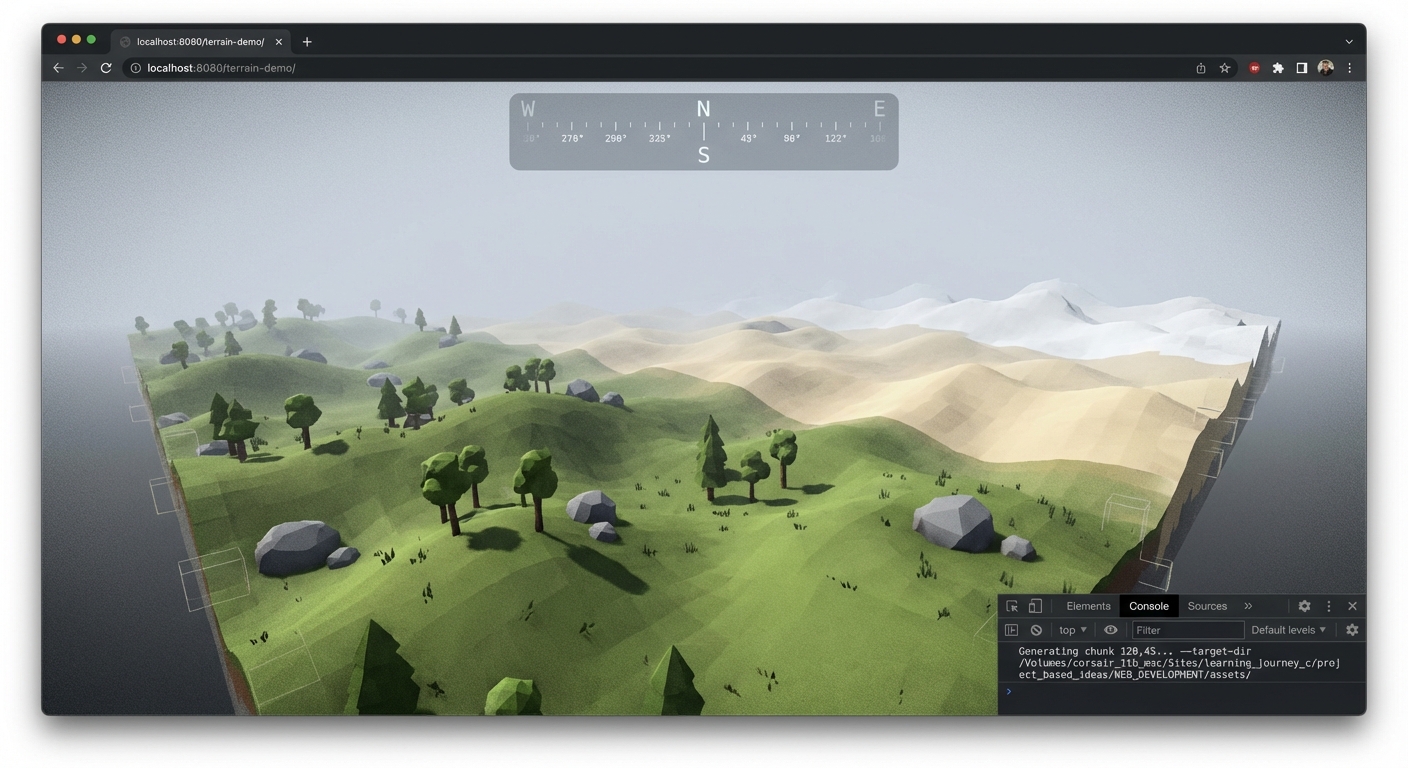
The Core Question You Are Answering
“How do you generate apparently endless terrain while keeping GPU and memory usage bounded?”
This matters because teams fail less from missing features and more from systems that cannot be reasoned about under change. This project trains you to design for predictability, instrumentation, and controlled growth.
Concepts You Must Understand First
- Deterministic Update Order
- Which systems run first, and what state do they own?
- Book Reference: “Texturing and Modeling: A Procedural Approach” by Ebert et al.
- Resource Lifecycle Management
- When is data loaded, retained, and evicted?
- Book Reference: “Game Engine Architecture” by Jason Gregory - resource chapters
- Event and Message Boundaries
- Which events are domain events versus UI-only events?
- Book Reference: “Game Programming Patterns” by Robert Nystrom - event queue chapter
- Profiling and Telemetry
- Which metrics prove correctness and performance?
- Book Reference: “Real-Time Rendering” by Akenine-Moller - optimization chapters
Questions to Guide Your Design
- Which state is authoritative, and which state is a derived view?
- What is your fixed-step versus variable-step policy?
- How will you prove subsystem isolation during a failure test?
- What are your frame-time and memory budgets for this project?
- How will you detect regression automatically after adding a new feature?
Thinking Exercise
Exercise: Failure Budget Tabletop
Create a table with three scenarios: latency spike, memory spike, and event storm. For each scenario, trace the exact subsystem boundary where the issue should be contained, the metric that detects it first, and the expected recovery strategy.
Questions to answer:
- Which invariant breaks first in each scenario?
- Which recovery action is safe during the current frame?
- Which signals prove the system returned to healthy state?
The Interview Questions They Will Ask
- “How did you decide system boundaries in this project?”
- “Which metrics did you track to prove the architecture works?”
- “How do you reproduce and debug a non-deterministic bug in real time systems?”
- “What tradeoffs did you make between abstraction and performance?”
- “How would this design evolve if user count or world size doubled?”
Hints in Layers
Hint 1: Start with contracts, not features Write a one-page runtime contract defining ownership, ordering, and lifecycle before implementation.
Hint 2: Instrument early Add telemetry from day one so regressions are visible while the system is still small.
Hint 3: Add controlled failure injection Introduce toggles that simulate delays or dropped events to validate resilience.
Hint 4: Validate with repeatable scripts Use a deterministic scenario playback to compare metrics before and after each change.
Books That Will Help
| Topic | Book | Chapter |
|---|---|---|
| Runtime design | “Texturing and Modeling: A Procedural Approach” by Ebert et al. | Relevant architecture chapters |
| Performance diagnostics | “Real-Time Rendering” by Akenine-Moller | Pipeline optimization chapters |
| System boundaries | “Game Programming Patterns” by Robert Nystrom | Update, event queue, state |
Common Pitfalls and Debugging
Problem 1: “Behavior differs between runs”
- Why: Update ordering or hidden mutable state is non-deterministic.
- Fix: Enforce deterministic ordering and isolate mutable ownership.
- Quick test: Replay the same deterministic input stream twice and diff telemetry output.
Problem 2: “Performance fixes break correctness”
- Why: Optimizations bypassed invariant checks.
- Fix: Keep invariants explicit and validate them after each optimization pass.
- Quick test: Run correctness assertions with optimization toggles on and off.
Problem 3: “Memory keeps growing”
- Why: Resource eviction policies are missing or too conservative.
- Fix: Add lifecycle states and eviction thresholds tied to scene scope.
- Quick test: Run a long session, capture memory high-water marks, and verify plateau behavior.
Definition of Done
- Core functionality demonstrates Procedural World Generation at Scale in a realistic scenario
- Deterministic replay script produces stable outcomes
- Telemetry panel exposes frame, memory, and subsystem timings
- At least one controlled failure injection path is implemented and documented
- Recovery path succeeds without full application restart
- Performance budget stays within documented limits on reference hardware
- Architecture and invariants are documented in a short design note
Project 19: Build a Stylized Shader Lab (Toon, Water, Fire)
- File: P19-stylized-shader-lab.md
- Main Programming Language: TypeScript
- Alternative Programming Languages: JavaScript, Rust (WASM), C# (Unity prototype parity)
- Coolness Level: 5 - Legendary
- Business Potential: 3 - Niche but high differentiation
- Difficulty: Expert
- Knowledge Area: Rendering Shaders
- Software or Tool: GLSL + Three.js ShaderMaterial
- Main Book: “The Book of Shaders” by Gonzalez Vivo and Lowe
What you will build: A production-style module centered on Custom Shader Mastery and Stylized Rendering with observable runtime output and measurable correctness signals.
Why it teaches Three.js: It forces you to treat Three.js as a systems runtime, not just a rendering library, by implementing Vertex displacement, fragment lighting models, signed distance shaping, shadow sampling, depth textures, and framebuffer feedback loops.
Core challenges you will face:
- Boundary design under pressure -> You must keep modules isolated while features grow.
- Runtime correctness verification -> You need explicit invariants and failure tests.
- Performance and operability tradeoffs -> Every abstraction choice affects frame time and memory.
Real World Outcome
When you open the project, you see a functional scenario proving the concept end-to-end, not a toy placeholder. The UI includes a diagnostics panel with frame time, subsystem timings, memory usage, and critical state transitions. Interactions are observable: toggling a subsystem shows measurable impact, failure injection demonstrates recovery behavior, and logs annotate the exact phase where work happened. The project includes a repeatable walkthrough document so a reviewer can run the same sequence and confirm identical outcomes. By the end, you can demonstrate stable behavior under normal load, controlled degradation under stress, and a clear explanation of why the architecture holds.
Observable session transcript (example):
action: boot project result: all subsystem health checks green action: run stress preset result: frame time rises from 11.4ms to 15.8ms, no dropped simulation ticks action: enable debug overlays result: timing histogram and queue depth visible in HUD action: trigger recovery test result: degraded subsystem is isolated and recovers without full restart
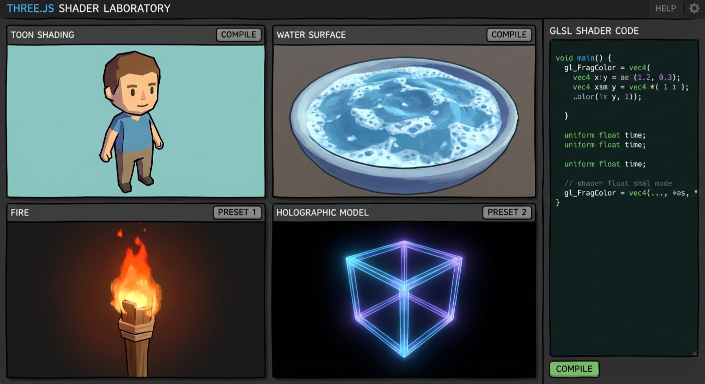
The Core Question You Are Answering
“How do you design a repeatable shader workflow that scales from prototypes to production visuals?”
This matters because teams fail less from missing features and more from systems that cannot be reasoned about under change. This project trains you to design for predictability, instrumentation, and controlled growth.
Concepts You Must Understand First
- Deterministic Update Order
- Which systems run first, and what state do they own?
- Book Reference: “The Book of Shaders” by Gonzalez Vivo and Lowe
- Resource Lifecycle Management
- When is data loaded, retained, and evicted?
- Book Reference: “Game Engine Architecture” by Jason Gregory - resource chapters
- Event and Message Boundaries
- Which events are domain events versus UI-only events?
- Book Reference: “Game Programming Patterns” by Robert Nystrom - event queue chapter
- Profiling and Telemetry
- Which metrics prove correctness and performance?
- Book Reference: “Real-Time Rendering” by Akenine-Moller - optimization chapters
Questions to Guide Your Design
- Which state is authoritative, and which state is a derived view?
- What is your fixed-step versus variable-step policy?
- How will you prove subsystem isolation during a failure test?
- What are your frame-time and memory budgets for this project?
- How will you detect regression automatically after adding a new feature?
Thinking Exercise
Exercise: Failure Budget Tabletop
Create a table with three scenarios: latency spike, memory spike, and event storm. For each scenario, trace the exact subsystem boundary where the issue should be contained, the metric that detects it first, and the expected recovery strategy.
Questions to answer:
- Which invariant breaks first in each scenario?
- Which recovery action is safe during the current frame?
- Which signals prove the system returned to healthy state?
The Interview Questions They Will Ask
- “How did you decide system boundaries in this project?”
- “Which metrics did you track to prove the architecture works?”
- “How do you reproduce and debug a non-deterministic bug in real time systems?”
- “What tradeoffs did you make between abstraction and performance?”
- “How would this design evolve if user count or world size doubled?”
Hints in Layers
Hint 1: Start with contracts, not features Write a one-page runtime contract defining ownership, ordering, and lifecycle before implementation.
Hint 2: Instrument early Add telemetry from day one so regressions are visible while the system is still small.
Hint 3: Add controlled failure injection Introduce toggles that simulate delays or dropped events to validate resilience.
Hint 4: Validate with repeatable scripts Use a deterministic scenario playback to compare metrics before and after each change.
Books That Will Help
| Topic | Book | Chapter |
|---|---|---|
| Runtime design | “The Book of Shaders” by Gonzalez Vivo and Lowe | Relevant architecture chapters |
| Performance diagnostics | “Real-Time Rendering” by Akenine-Moller | Pipeline optimization chapters |
| System boundaries | “Game Programming Patterns” by Robert Nystrom | Update, event queue, state |
Common Pitfalls and Debugging
Problem 1: “Behavior differs between runs”
- Why: Update ordering or hidden mutable state is non-deterministic.
- Fix: Enforce deterministic ordering and isolate mutable ownership.
- Quick test: Replay the same deterministic input stream twice and diff telemetry output.
Problem 2: “Performance fixes break correctness”
- Why: Optimizations bypassed invariant checks.
- Fix: Keep invariants explicit and validate them after each optimization pass.
- Quick test: Run correctness assertions with optimization toggles on and off.
Problem 3: “Memory keeps growing”
- Why: Resource eviction policies are missing or too conservative.
- Fix: Add lifecycle states and eviction thresholds tied to scene scope.
- Quick test: Run a long session, capture memory high-water marks, and verify plateau behavior.
Definition of Done
- Core functionality demonstrates Custom Shader Mastery and Stylized Rendering in a realistic scenario
- Deterministic replay script produces stable outcomes
- Telemetry panel exposes frame, memory, and subsystem timings
- At least one controlled failure injection path is implemented and documented
- Recovery path succeeds without full application restart
- Performance budget stays within documented limits on reference hardware
- Architecture and invariants are documented in a short design note
Project 20: Build a Post-Processing Engine without EffectComposer
- File: P20-postprocessing-engine-from-scratch.md
- Main Programming Language: TypeScript
- Alternative Programming Languages: JavaScript, Rust (WASM), C# (Unity prototype parity)
- Coolness Level: 5 - Legendary
- Business Potential: 4 - Strong product fit
- Difficulty: Expert
- Knowledge Area: Post Processing
- Software or Tool: Three.js WebGLRenderTarget + custom pass chain
- Main Book: “Real-Time Rendering” by Akenine-Moller - post effects chapters
What you will build: A production-style module centered on Post-Processing Pipeline Engineering with observable runtime output and measurable correctness signals.
Why it teaches Three.js: It forces you to treat Three.js as a systems runtime, not just a rendering library, by implementing Render targets, custom pass scheduler, ping-pong buffers, HDR luminance extraction, bloom kernels, SSAO sampling, and tone mapping.
Core challenges you will face:
- Boundary design under pressure -> You must keep modules isolated while features grow.
- Runtime correctness verification -> You need explicit invariants and failure tests.
- Performance and operability tradeoffs -> Every abstraction choice affects frame time and memory.
Real World Outcome
When you open the project, you see a functional scenario proving the concept end-to-end, not a toy placeholder. The UI includes a diagnostics panel with frame time, subsystem timings, memory usage, and critical state transitions. Interactions are observable: toggling a subsystem shows measurable impact, failure injection demonstrates recovery behavior, and logs annotate the exact phase where work happened. The project includes a repeatable walkthrough document so a reviewer can run the same sequence and confirm identical outcomes. By the end, you can demonstrate stable behavior under normal load, controlled degradation under stress, and a clear explanation of why the architecture holds.
Observable session transcript (example):
action: boot project result: all subsystem health checks green action: run stress preset result: frame time rises from 11.4ms to 15.8ms, no dropped simulation ticks action: enable debug overlays result: timing histogram and queue depth visible in HUD action: trigger recovery test result: degraded subsystem is isolated and recovers without full restart
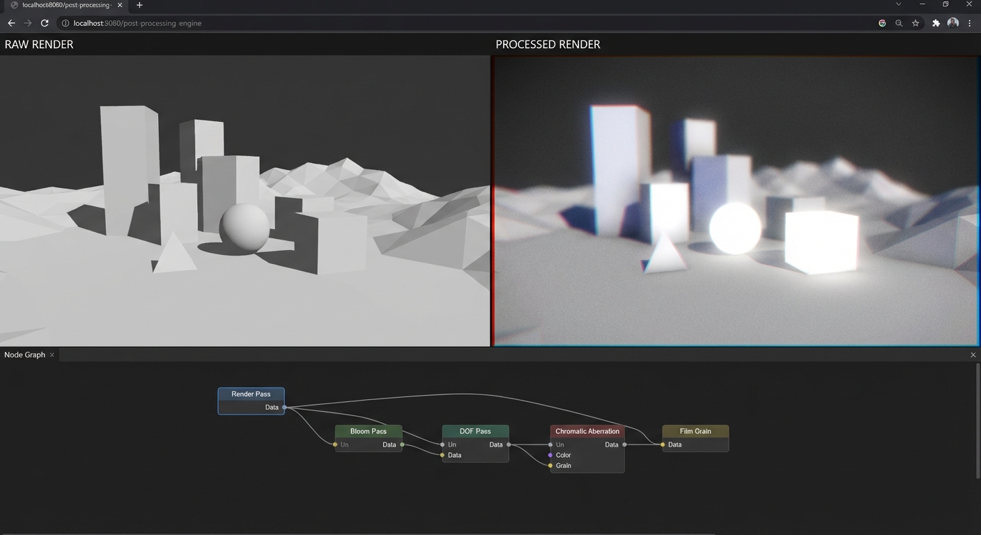
The Core Question You Are Answering
“What actually happens between scene render and final color when you build the pipeline yourself?”
This matters because teams fail less from missing features and more from systems that cannot be reasoned about under change. This project trains you to design for predictability, instrumentation, and controlled growth.
Concepts You Must Understand First
- Deterministic Update Order
- Which systems run first, and what state do they own?
- Book Reference: “Real-Time Rendering” by Akenine-Moller - post effects chapters
- Resource Lifecycle Management
- When is data loaded, retained, and evicted?
- Book Reference: “Game Engine Architecture” by Jason Gregory - resource chapters
- Event and Message Boundaries
- Which events are domain events versus UI-only events?
- Book Reference: “Game Programming Patterns” by Robert Nystrom - event queue chapter
- Profiling and Telemetry
- Which metrics prove correctness and performance?
- Book Reference: “Real-Time Rendering” by Akenine-Moller - optimization chapters
Questions to Guide Your Design
- Which state is authoritative, and which state is a derived view?
- What is your fixed-step versus variable-step policy?
- How will you prove subsystem isolation during a failure test?
- What are your frame-time and memory budgets for this project?
- How will you detect regression automatically after adding a new feature?
Thinking Exercise
Exercise: Failure Budget Tabletop
Create a table with three scenarios: latency spike, memory spike, and event storm. For each scenario, trace the exact subsystem boundary where the issue should be contained, the metric that detects it first, and the expected recovery strategy.
Questions to answer:
- Which invariant breaks first in each scenario?
- Which recovery action is safe during the current frame?
- Which signals prove the system returned to healthy state?
The Interview Questions They Will Ask
- “How did you decide system boundaries in this project?”
- “Which metrics did you track to prove the architecture works?”
- “How do you reproduce and debug a non-deterministic bug in real time systems?”
- “What tradeoffs did you make between abstraction and performance?”
- “How would this design evolve if user count or world size doubled?”
Hints in Layers
Hint 1: Start with contracts, not features Write a one-page runtime contract defining ownership, ordering, and lifecycle before implementation.
Hint 2: Instrument early Add telemetry from day one so regressions are visible while the system is still small.
Hint 3: Add controlled failure injection Introduce toggles that simulate delays or dropped events to validate resilience.
Hint 4: Validate with repeatable scripts Use a deterministic scenario playback to compare metrics before and after each change.
Books That Will Help
| Topic | Book | Chapter |
|---|---|---|
| Runtime design | “Real-Time Rendering” by Akenine-Moller - post effects chapters | Relevant architecture chapters |
| Performance diagnostics | “Real-Time Rendering” by Akenine-Moller | Pipeline optimization chapters |
| System boundaries | “Game Programming Patterns” by Robert Nystrom | Update, event queue, state |
Common Pitfalls and Debugging
Problem 1: “Behavior differs between runs”
- Why: Update ordering or hidden mutable state is non-deterministic.
- Fix: Enforce deterministic ordering and isolate mutable ownership.
- Quick test: Replay the same deterministic input stream twice and diff telemetry output.
Problem 2: “Performance fixes break correctness”
- Why: Optimizations bypassed invariant checks.
- Fix: Keep invariants explicit and validate them after each optimization pass.
- Quick test: Run correctness assertions with optimization toggles on and off.
Problem 3: “Memory keeps growing”
- Why: Resource eviction policies are missing or too conservative.
- Fix: Add lifecycle states and eviction thresholds tied to scene scope.
- Quick test: Run a long session, capture memory high-water marks, and verify plateau behavior.
Definition of Done
- Core functionality demonstrates Post-Processing Pipeline Engineering in a realistic scenario
- Deterministic replay script produces stable outcomes
- Telemetry panel exposes frame, memory, and subsystem timings
- At least one controlled failure injection path is implemented and documented
- Recovery path succeeds without full application restart
- Performance budget stays within documented limits on reference hardware
- Architecture and invariants are documented in a short design note
Project 21: Optimize a Heavy Scene to 60 FPS on Mobile
- File: P21-mobile-60fps-performance-lab.md
- Main Programming Language: TypeScript
- Alternative Programming Languages: JavaScript, Rust (WASM), C# (Unity prototype parity)
- Coolness Level: 5 - Legendary
- Business Potential: 5 - High monetization potential
- Difficulty: Advanced
- Knowledge Area: Performance
- Software or Tool: Three.js + Spector.js + browser performance tools
- Main Book: “Real-Time Rendering” by Akenine-Moller - optimization chapters
What you will build: A production-style module centered on Performance Engineering for Mobile 60 FPS with observable runtime output and measurable correctness signals.
Why it teaches Three.js: It forces you to treat Three.js as a systems runtime, not just a rendering library, by implementing Draw call budgeting, instancing, texture atlas strategy, adaptive resolution, profiling workflow, thermal guardrails, and quality tiers.
Core challenges you will face:
- Boundary design under pressure -> You must keep modules isolated while features grow.
- Runtime correctness verification -> You need explicit invariants and failure tests.
- Performance and operability tradeoffs -> Every abstraction choice affects frame time and memory.
Real World Outcome
When you open the project, you see a functional scenario proving the concept end-to-end, not a toy placeholder. The UI includes a diagnostics panel with frame time, subsystem timings, memory usage, and critical state transitions. Interactions are observable: toggling a subsystem shows measurable impact, failure injection demonstrates recovery behavior, and logs annotate the exact phase where work happened. The project includes a repeatable walkthrough document so a reviewer can run the same sequence and confirm identical outcomes. By the end, you can demonstrate stable behavior under normal load, controlled degradation under stress, and a clear explanation of why the architecture holds.
Observable session transcript (example):
action: boot project result: all subsystem health checks green action: run stress preset result: frame time rises from 11.4ms to 15.8ms, no dropped simulation ticks action: enable debug overlays result: timing histogram and queue depth visible in HUD action: trigger recovery test result: degraded subsystem is isolated and recovers without full restart
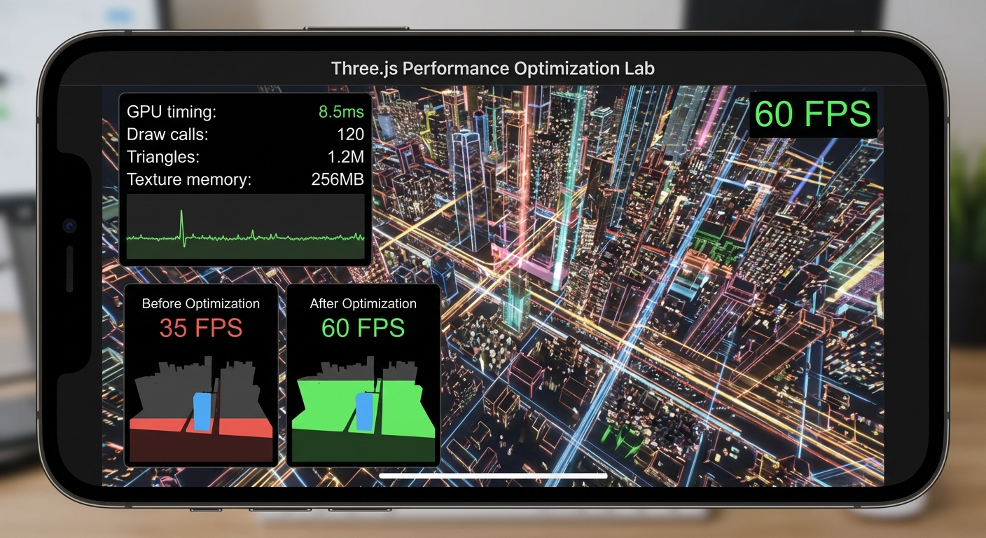
The Core Question You Are Answering
“How do you create a measurable optimization process that survives real device constraints?”
This matters because teams fail less from missing features and more from systems that cannot be reasoned about under change. This project trains you to design for predictability, instrumentation, and controlled growth.
Concepts You Must Understand First
- Deterministic Update Order
- Which systems run first, and what state do they own?
- Book Reference: “Real-Time Rendering” by Akenine-Moller - optimization chapters
- Resource Lifecycle Management
- When is data loaded, retained, and evicted?
- Book Reference: “Game Engine Architecture” by Jason Gregory - resource chapters
- Event and Message Boundaries
- Which events are domain events versus UI-only events?
- Book Reference: “Game Programming Patterns” by Robert Nystrom - event queue chapter
- Profiling and Telemetry
- Which metrics prove correctness and performance?
- Book Reference: “Real-Time Rendering” by Akenine-Moller - optimization chapters
Questions to Guide Your Design
- Which state is authoritative, and which state is a derived view?
- What is your fixed-step versus variable-step policy?
- How will you prove subsystem isolation during a failure test?
- What are your frame-time and memory budgets for this project?
- How will you detect regression automatically after adding a new feature?
Thinking Exercise
Exercise: Failure Budget Tabletop
Create a table with three scenarios: latency spike, memory spike, and event storm. For each scenario, trace the exact subsystem boundary where the issue should be contained, the metric that detects it first, and the expected recovery strategy.
Questions to answer:
- Which invariant breaks first in each scenario?
- Which recovery action is safe during the current frame?
- Which signals prove the system returned to healthy state?
The Interview Questions They Will Ask
- “How did you decide system boundaries in this project?”
- “Which metrics did you track to prove the architecture works?”
- “How do you reproduce and debug a non-deterministic bug in real time systems?”
- “What tradeoffs did you make between abstraction and performance?”
- “How would this design evolve if user count or world size doubled?”
Hints in Layers
Hint 1: Start with contracts, not features Write a one-page runtime contract defining ownership, ordering, and lifecycle before implementation.
Hint 2: Instrument early Add telemetry from day one so regressions are visible while the system is still small.
Hint 3: Add controlled failure injection Introduce toggles that simulate delays or dropped events to validate resilience.
Hint 4: Validate with repeatable scripts Use a deterministic scenario playback to compare metrics before and after each change.
Books That Will Help
| Topic | Book | Chapter |
|---|---|---|
| Runtime design | “Real-Time Rendering” by Akenine-Moller - optimization chapters | Relevant architecture chapters |
| Performance diagnostics | “Real-Time Rendering” by Akenine-Moller | Pipeline optimization chapters |
| System boundaries | “Game Programming Patterns” by Robert Nystrom | Update, event queue, state |
Common Pitfalls and Debugging
Problem 1: “Behavior differs between runs”
- Why: Update ordering or hidden mutable state is non-deterministic.
- Fix: Enforce deterministic ordering and isolate mutable ownership.
- Quick test: Replay the same deterministic input stream twice and diff telemetry output.
Problem 2: “Performance fixes break correctness”
- Why: Optimizations bypassed invariant checks.
- Fix: Keep invariants explicit and validate them after each optimization pass.
- Quick test: Run correctness assertions with optimization toggles on and off.
Problem 3: “Memory keeps growing”
- Why: Resource eviction policies are missing or too conservative.
- Fix: Add lifecycle states and eviction thresholds tied to scene scope.
- Quick test: Run a long session, capture memory high-water marks, and verify plateau behavior.
Definition of Done
- Core functionality demonstrates Performance Engineering for Mobile 60 FPS in a realistic scenario
- Deterministic replay script produces stable outcomes
- Telemetry panel exposes frame, memory, and subsystem timings
- At least one controlled failure injection path is implemented and documented
- Recovery path succeeds without full application restart
- Performance budget stays within documented limits on reference hardware
- Architecture and invariants are documented in a short design note
Project 22: Build a WebXR VR Room with Hand and AR Interaction
- File: P22-webxr-vr-ar-room.md
- Main Programming Language: TypeScript
- Alternative Programming Languages: JavaScript, Rust (WASM), C# (Unity prototype parity)
- Coolness Level: 5 - Legendary
- Business Potential: 4 - Strong product fit
- Difficulty: Expert
- Knowledge Area: XR
- Software or Tool: Three.js WebXR + WebXR Device API
- Main Book: “WebXR Explainer” and official W3C/WebXR specs
What you will build: A production-style module centered on WebXR VR and AR Systems with observable runtime output and measurable correctness signals.
Why it teaches Three.js: It forces you to treat Three.js as a systems runtime, not just a rendering library, by implementing WebXR session lifecycle, controller and hand input mapping, teleport locomotion, frame pacing, AR hit testing, anchors, and comfort constraints.
Core challenges you will face:
- Boundary design under pressure -> You must keep modules isolated while features grow.
- Runtime correctness verification -> You need explicit invariants and failure tests.
- Performance and operability tradeoffs -> Every abstraction choice affects frame time and memory.
Real World Outcome
When you open the project, you see a functional scenario proving the concept end-to-end, not a toy placeholder. The UI includes a diagnostics panel with frame time, subsystem timings, memory usage, and critical state transitions. Interactions are observable: toggling a subsystem shows measurable impact, failure injection demonstrates recovery behavior, and logs annotate the exact phase where work happened. The project includes a repeatable walkthrough document so a reviewer can run the same sequence and confirm identical outcomes. By the end, you can demonstrate stable behavior under normal load, controlled degradation under stress, and a clear explanation of why the architecture holds.
Observable session transcript (example):
action: boot project result: all subsystem health checks green action: run stress preset result: frame time rises from 11.4ms to 15.8ms, no dropped simulation ticks action: enable debug overlays result: timing histogram and queue depth visible in HUD action: trigger recovery test result: degraded subsystem is isolated and recovers without full restart
The Core Question You Are Answering
“How do you ship one interaction model that works across immersive VR and handheld AR modes?”
This matters because teams fail less from missing features and more from systems that cannot be reasoned about under change. This project trains you to design for predictability, instrumentation, and controlled growth.
Concepts You Must Understand First
- Deterministic Update Order
- Which systems run first, and what state do they own?
- Book Reference: “WebXR Explainer” and official W3C/WebXR specs
- Resource Lifecycle Management
- When is data loaded, retained, and evicted?
- Book Reference: “Game Engine Architecture” by Jason Gregory - resource chapters
- Event and Message Boundaries
- Which events are domain events versus UI-only events?
- Book Reference: “Game Programming Patterns” by Robert Nystrom - event queue chapter
- Profiling and Telemetry
- Which metrics prove correctness and performance?
- Book Reference: “Real-Time Rendering” by Akenine-Moller - optimization chapters
Questions to Guide Your Design
- Which state is authoritative, and which state is a derived view?
- What is your fixed-step versus variable-step policy?
- How will you prove subsystem isolation during a failure test?
- What are your frame-time and memory budgets for this project?
- How will you detect regression automatically after adding a new feature?
Thinking Exercise
Exercise: Failure Budget Tabletop
Create a table with three scenarios: latency spike, memory spike, and event storm. For each scenario, trace the exact subsystem boundary where the issue should be contained, the metric that detects it first, and the expected recovery strategy.
Questions to answer:
- Which invariant breaks first in each scenario?
- Which recovery action is safe during the current frame?
- Which signals prove the system returned to healthy state?
The Interview Questions They Will Ask
- “How did you decide system boundaries in this project?”
- “Which metrics did you track to prove the architecture works?”
- “How do you reproduce and debug a non-deterministic bug in real time systems?”
- “What tradeoffs did you make between abstraction and performance?”
- “How would this design evolve if user count or world size doubled?”
Hints in Layers
Hint 1: Start with contracts, not features Write a one-page runtime contract defining ownership, ordering, and lifecycle before implementation.
Hint 2: Instrument early Add telemetry from day one so regressions are visible while the system is still small.
Hint 3: Add controlled failure injection Introduce toggles that simulate delays or dropped events to validate resilience.
Hint 4: Validate with repeatable scripts Use a deterministic scenario playback to compare metrics before and after each change.
Books That Will Help
| Topic | Book | Chapter |
|---|---|---|
| Runtime design | “WebXR Explainer” and official W3C/WebXR specs | Relevant architecture chapters |
| Performance diagnostics | “Real-Time Rendering” by Akenine-Moller | Pipeline optimization chapters |
| System boundaries | “Game Programming Patterns” by Robert Nystrom | Update, event queue, state |
Common Pitfalls and Debugging
Problem 1: “Behavior differs between runs”
- Why: Update ordering or hidden mutable state is non-deterministic.
- Fix: Enforce deterministic ordering and isolate mutable ownership.
- Quick test: Replay the same deterministic input stream twice and diff telemetry output.
Problem 2: “Performance fixes break correctness”
- Why: Optimizations bypassed invariant checks.
- Fix: Keep invariants explicit and validate them after each optimization pass.
- Quick test: Run correctness assertions with optimization toggles on and off.
Problem 3: “Memory keeps growing”
- Why: Resource eviction policies are missing or too conservative.
- Fix: Add lifecycle states and eviction thresholds tied to scene scope.
- Quick test: Run a long session, capture memory high-water marks, and verify plateau behavior.
Definition of Done
- Core functionality demonstrates WebXR VR and AR Systems in a realistic scenario
- Deterministic replay script produces stable outcomes
- Telemetry panel exposes frame, memory, and subsystem timings
- At least one controlled failure injection path is implemented and documented
- Recovery path succeeds without full application restart
- Performance budget stays within documented limits on reference hardware
- Architecture and invariants are documented in a short design note
Project 23: Build a Full Asset Pipeline from Blender to Three.js
- File: P23-blender-to-threejs-asset-pipeline.md
- Main Programming Language: TypeScript
- Alternative Programming Languages: JavaScript, Rust (WASM), C# (Unity prototype parity)
- Coolness Level: 4 - Impressive
- Business Potential: 5 - High monetization potential
- Difficulty: Advanced
- Knowledge Area: Asset Pipeline
- Software or Tool: Blender + glTF tools + CDN
- Main Book: “Digital Content Creation Pipeline” references and Khronos docs
What you will build: A production-style module centered on Production Asset Pipeline: Blender to Runtime with observable runtime output and measurable correctness signals.
Why it teaches Three.js: It forces you to treat Three.js as a systems runtime, not just a rendering library, by implementing DCC naming standards, GLTF export settings, Draco and KTX2 compression, baking strategy, semantic versioning, CDN cache policy, and rollback safety.
Core challenges you will face:
- Boundary design under pressure -> You must keep modules isolated while features grow.
- Runtime correctness verification -> You need explicit invariants and failure tests.
- Performance and operability tradeoffs -> Every abstraction choice affects frame time and memory.
Real World Outcome
When you open the project, you see a functional scenario proving the concept end-to-end, not a toy placeholder. The UI includes a diagnostics panel with frame time, subsystem timings, memory usage, and critical state transitions. Interactions are observable: toggling a subsystem shows measurable impact, failure injection demonstrates recovery behavior, and logs annotate the exact phase where work happened. The project includes a repeatable walkthrough document so a reviewer can run the same sequence and confirm identical outcomes. By the end, you can demonstrate stable behavior under normal load, controlled degradation under stress, and a clear explanation of why the architecture holds.
Observable session transcript (example):
action: boot project result: all subsystem health checks green action: run stress preset result: frame time rises from 11.4ms to 15.8ms, no dropped simulation ticks action: enable debug overlays result: timing histogram and queue depth visible in HUD action: trigger recovery test result: degraded subsystem is isolated and recovers without full restart
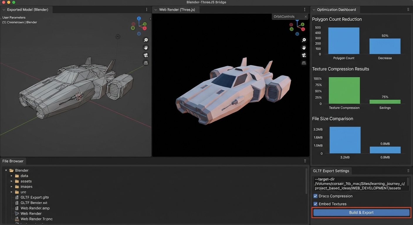
The Core Question You Are Answering
“How do you prevent content chaos and deliver predictable asset builds for teams?”
This matters because teams fail less from missing features and more from systems that cannot be reasoned about under change. This project trains you to design for predictability, instrumentation, and controlled growth.
Concepts You Must Understand First
- Deterministic Update Order
- Which systems run first, and what state do they own?
- Book Reference: “Digital Content Creation Pipeline” references and Khronos docs
- Resource Lifecycle Management
- When is data loaded, retained, and evicted?
- Book Reference: “Game Engine Architecture” by Jason Gregory - resource chapters
- Event and Message Boundaries
- Which events are domain events versus UI-only events?
- Book Reference: “Game Programming Patterns” by Robert Nystrom - event queue chapter
- Profiling and Telemetry
- Which metrics prove correctness and performance?
- Book Reference: “Real-Time Rendering” by Akenine-Moller - optimization chapters
Questions to Guide Your Design
- Which state is authoritative, and which state is a derived view?
- What is your fixed-step versus variable-step policy?
- How will you prove subsystem isolation during a failure test?
- What are your frame-time and memory budgets for this project?
- How will you detect regression automatically after adding a new feature?
Thinking Exercise
Exercise: Failure Budget Tabletop
Create a table with three scenarios: latency spike, memory spike, and event storm. For each scenario, trace the exact subsystem boundary where the issue should be contained, the metric that detects it first, and the expected recovery strategy.
Questions to answer:
- Which invariant breaks first in each scenario?
- Which recovery action is safe during the current frame?
- Which signals prove the system returned to healthy state?
The Interview Questions They Will Ask
- “How did you decide system boundaries in this project?”
- “Which metrics did you track to prove the architecture works?”
- “How do you reproduce and debug a non-deterministic bug in real time systems?”
- “What tradeoffs did you make between abstraction and performance?”
- “How would this design evolve if user count or world size doubled?”
Hints in Layers
Hint 1: Start with contracts, not features Write a one-page runtime contract defining ownership, ordering, and lifecycle before implementation.
Hint 2: Instrument early Add telemetry from day one so regressions are visible while the system is still small.
Hint 3: Add controlled failure injection Introduce toggles that simulate delays or dropped events to validate resilience.
Hint 4: Validate with repeatable scripts Use a deterministic scenario playback to compare metrics before and after each change.
Books That Will Help
| Topic | Book | Chapter |
|---|---|---|
| Runtime design | “Digital Content Creation Pipeline” references and Khronos docs | Relevant architecture chapters |
| Performance diagnostics | “Real-Time Rendering” by Akenine-Moller | Pipeline optimization chapters |
| System boundaries | “Game Programming Patterns” by Robert Nystrom | Update, event queue, state |
Common Pitfalls and Debugging
Problem 1: “Behavior differs between runs”
- Why: Update ordering or hidden mutable state is non-deterministic.
- Fix: Enforce deterministic ordering and isolate mutable ownership.
- Quick test: Replay the same deterministic input stream twice and diff telemetry output.
Problem 2: “Performance fixes break correctness”
- Why: Optimizations bypassed invariant checks.
- Fix: Keep invariants explicit and validate them after each optimization pass.
- Quick test: Run correctness assertions with optimization toggles on and off.
Problem 3: “Memory keeps growing”
- Why: Resource eviction policies are missing or too conservative.
- Fix: Add lifecycle states and eviction thresholds tied to scene scope.
- Quick test: Run a long session, capture memory high-water marks, and verify plateau behavior.
Definition of Done
- Core functionality demonstrates Production Asset Pipeline: Blender to Runtime in a realistic scenario
- Deterministic replay script produces stable outcomes
- Telemetry panel exposes frame, memory, and subsystem timings
- At least one controlled failure injection path is implemented and documented
- Recovery path succeeds without full application restart
- Performance budget stays within documented limits on reference hardware
- Architecture and invariants are documented in a short design note
Project 24: Implement a Dynamic Day/Night Lighting System
- File: P24-dynamic-day-night-lighting.md
- Main Programming Language: TypeScript
- Alternative Programming Languages: JavaScript, Rust (WASM), C# (Unity prototype parity)
- Coolness Level: 5 - Legendary
- Business Potential: 4 - Strong product fit
- Difficulty: Expert
- Knowledge Area: Lighting
- Software or Tool: Three.js + PMREM + shadow tuning
- Main Book: “Physically Based Rendering” references and RTR lighting chapters
What you will build: A production-style module centered on Advanced Lighting and Time-of-Day Systems with observable runtime output and measurable correctness signals.
Why it teaches Three.js: It forces you to treat Three.js as a systems runtime, not just a rendering library, by implementing Environment maps, IBL calibration, cascaded shadow maps, volumetric light shafts, probe blending, and weather-driven exposure curves.
Core challenges you will face:
- Boundary design under pressure -> You must keep modules isolated while features grow.
- Runtime correctness verification -> You need explicit invariants and failure tests.
- Performance and operability tradeoffs -> Every abstraction choice affects frame time and memory.
Real World Outcome
When you open the project, you see a functional scenario proving the concept end-to-end, not a toy placeholder. The UI includes a diagnostics panel with frame time, subsystem timings, memory usage, and critical state transitions. Interactions are observable: toggling a subsystem shows measurable impact, failure injection demonstrates recovery behavior, and logs annotate the exact phase where work happened. The project includes a repeatable walkthrough document so a reviewer can run the same sequence and confirm identical outcomes. By the end, you can demonstrate stable behavior under normal load, controlled degradation under stress, and a clear explanation of why the architecture holds.
Observable session transcript (example):
action: boot project result: all subsystem health checks green action: run stress preset result: frame time rises from 11.4ms to 15.8ms, no dropped simulation ticks action: enable debug overlays result: timing histogram and queue depth visible in HUD action: trigger recovery test result: degraded subsystem is isolated and recovers without full restart
The Core Question You Are Answering
“How do you maintain believable lighting continuity as sun position and atmosphere change over time?”
This matters because teams fail less from missing features and more from systems that cannot be reasoned about under change. This project trains you to design for predictability, instrumentation, and controlled growth.
Concepts You Must Understand First
- Deterministic Update Order
- Which systems run first, and what state do they own?
- Book Reference: “Physically Based Rendering” references and RTR lighting chapters
- Resource Lifecycle Management
- When is data loaded, retained, and evicted?
- Book Reference: “Game Engine Architecture” by Jason Gregory - resource chapters
- Event and Message Boundaries
- Which events are domain events versus UI-only events?
- Book Reference: “Game Programming Patterns” by Robert Nystrom - event queue chapter
- Profiling and Telemetry
- Which metrics prove correctness and performance?
- Book Reference: “Real-Time Rendering” by Akenine-Moller - optimization chapters
Questions to Guide Your Design
- Which state is authoritative, and which state is a derived view?
- What is your fixed-step versus variable-step policy?
- How will you prove subsystem isolation during a failure test?
- What are your frame-time and memory budgets for this project?
- How will you detect regression automatically after adding a new feature?
Thinking Exercise
Exercise: Failure Budget Tabletop
Create a table with three scenarios: latency spike, memory spike, and event storm. For each scenario, trace the exact subsystem boundary where the issue should be contained, the metric that detects it first, and the expected recovery strategy.
Questions to answer:
- Which invariant breaks first in each scenario?
- Which recovery action is safe during the current frame?
- Which signals prove the system returned to healthy state?
The Interview Questions They Will Ask
- “How did you decide system boundaries in this project?”
- “Which metrics did you track to prove the architecture works?”
- “How do you reproduce and debug a non-deterministic bug in real time systems?”
- “What tradeoffs did you make between abstraction and performance?”
- “How would this design evolve if user count or world size doubled?”
Hints in Layers
Hint 1: Start with contracts, not features Write a one-page runtime contract defining ownership, ordering, and lifecycle before implementation.
Hint 2: Instrument early Add telemetry from day one so regressions are visible while the system is still small.
Hint 3: Add controlled failure injection Introduce toggles that simulate delays or dropped events to validate resilience.
Hint 4: Validate with repeatable scripts Use a deterministic scenario playback to compare metrics before and after each change.
Books That Will Help
| Topic | Book | Chapter |
|---|---|---|
| Runtime design | “Physically Based Rendering” references and RTR lighting chapters | Relevant architecture chapters |
| Performance diagnostics | “Real-Time Rendering” by Akenine-Moller | Pipeline optimization chapters |
| System boundaries | “Game Programming Patterns” by Robert Nystrom | Update, event queue, state |
Common Pitfalls and Debugging
Problem 1: “Behavior differs between runs”
- Why: Update ordering or hidden mutable state is non-deterministic.
- Fix: Enforce deterministic ordering and isolate mutable ownership.
- Quick test: Replay the same deterministic input stream twice and diff telemetry output.
Problem 2: “Performance fixes break correctness”
- Why: Optimizations bypassed invariant checks.
- Fix: Keep invariants explicit and validate them after each optimization pass.
- Quick test: Run correctness assertions with optimization toggles on and off.
Problem 3: “Memory keeps growing”
- Why: Resource eviction policies are missing or too conservative.
- Fix: Add lifecycle states and eviction thresholds tied to scene scope.
- Quick test: Run a long session, capture memory high-water marks, and verify plateau behavior.
Definition of Done
- Core functionality demonstrates Advanced Lighting and Time-of-Day Systems in a realistic scenario
- Deterministic replay script produces stable outcomes
- Telemetry panel exposes frame, memory, and subsystem timings
- At least one controlled failure injection path is implemented and documented
- Recovery path succeeds without full application restart
- Performance budget stays within documented limits on reference hardware
- Architecture and invariants are documented in a short design note
Project 25: Build an In-World UI + HUD Integration System
- File: P25-in-world-ui-system.md
- Main Programming Language: TypeScript
- Alternative Programming Languages: JavaScript, Rust (WASM), C# (Unity prototype parity)
- Coolness Level: 4 - Impressive
- Business Potential: 4 - Strong product fit
- Difficulty: Advanced
- Knowledge Area: 3D UI
- Software or Tool: Three.js + CSS2D/CSS3D + UI state manager
- Main Book: “Designing Interfaces” patterns adapted to spatial UI
What you will build: A production-style module centered on 3D UI Architecture and Interaction Design with observable runtime output and measurable correctness signals.
Why it teaches Three.js: It forces you to treat Three.js as a systems runtime, not just a rendering library, by implementing 3D panel layout, raycast interaction, HTML overlay synchronization, focus routing, readability scaling, and responsive XR-safe UI composition.
Core challenges you will face:
- Boundary design under pressure -> You must keep modules isolated while features grow.
- Runtime correctness verification -> You need explicit invariants and failure tests.
- Performance and operability tradeoffs -> Every abstraction choice affects frame time and memory.
Real World Outcome
When you open the project, you see a functional scenario proving the concept end-to-end, not a toy placeholder. The UI includes a diagnostics panel with frame time, subsystem timings, memory usage, and critical state transitions. Interactions are observable: toggling a subsystem shows measurable impact, failure injection demonstrates recovery behavior, and logs annotate the exact phase where work happened. The project includes a repeatable walkthrough document so a reviewer can run the same sequence and confirm identical outcomes. By the end, you can demonstrate stable behavior under normal load, controlled degradation under stress, and a clear explanation of why the architecture holds.
Observable session transcript (example):
action: boot project result: all subsystem health checks green action: run stress preset result: frame time rises from 11.4ms to 15.8ms, no dropped simulation ticks action: enable debug overlays result: timing histogram and queue depth visible in HUD action: trigger recovery test result: degraded subsystem is isolated and recovers without full restart
The Core Question You Are Answering
“How do you combine DOM and world-space UI without broken input or visual drift?”
This matters because teams fail less from missing features and more from systems that cannot be reasoned about under change. This project trains you to design for predictability, instrumentation, and controlled growth.
Concepts You Must Understand First
- Deterministic Update Order
- Which systems run first, and what state do they own?
- Book Reference: “Designing Interfaces” patterns adapted to spatial UI
- Resource Lifecycle Management
- When is data loaded, retained, and evicted?
- Book Reference: “Game Engine Architecture” by Jason Gregory - resource chapters
- Event and Message Boundaries
- Which events are domain events versus UI-only events?
- Book Reference: “Game Programming Patterns” by Robert Nystrom - event queue chapter
- Profiling and Telemetry
- Which metrics prove correctness and performance?
- Book Reference: “Real-Time Rendering” by Akenine-Moller - optimization chapters
Questions to Guide Your Design
- Which state is authoritative, and which state is a derived view?
- What is your fixed-step versus variable-step policy?
- How will you prove subsystem isolation during a failure test?
- What are your frame-time and memory budgets for this project?
- How will you detect regression automatically after adding a new feature?
Thinking Exercise
Exercise: Failure Budget Tabletop
Create a table with three scenarios: latency spike, memory spike, and event storm. For each scenario, trace the exact subsystem boundary where the issue should be contained, the metric that detects it first, and the expected recovery strategy.
Questions to answer:
- Which invariant breaks first in each scenario?
- Which recovery action is safe during the current frame?
- Which signals prove the system returned to healthy state?
The Interview Questions They Will Ask
- “How did you decide system boundaries in this project?”
- “Which metrics did you track to prove the architecture works?”
- “How do you reproduce and debug a non-deterministic bug in real time systems?”
- “What tradeoffs did you make between abstraction and performance?”
- “How would this design evolve if user count or world size doubled?”
Hints in Layers
Hint 1: Start with contracts, not features Write a one-page runtime contract defining ownership, ordering, and lifecycle before implementation.
Hint 2: Instrument early Add telemetry from day one so regressions are visible while the system is still small.
Hint 3: Add controlled failure injection Introduce toggles that simulate delays or dropped events to validate resilience.
Hint 4: Validate with repeatable scripts Use a deterministic scenario playback to compare metrics before and after each change.
Books That Will Help
| Topic | Book | Chapter |
|---|---|---|
| Runtime design | “Designing Interfaces” patterns adapted to spatial UI | Relevant architecture chapters |
| Performance diagnostics | “Real-Time Rendering” by Akenine-Moller | Pipeline optimization chapters |
| System boundaries | “Game Programming Patterns” by Robert Nystrom | Update, event queue, state |
Common Pitfalls and Debugging
Problem 1: “Behavior differs between runs”
- Why: Update ordering or hidden mutable state is non-deterministic.
- Fix: Enforce deterministic ordering and isolate mutable ownership.
- Quick test: Replay the same deterministic input stream twice and diff telemetry output.
Problem 2: “Performance fixes break correctness”
- Why: Optimizations bypassed invariant checks.
- Fix: Keep invariants explicit and validate them after each optimization pass.
- Quick test: Run correctness assertions with optimization toggles on and off.
Problem 3: “Memory keeps growing”
- Why: Resource eviction policies are missing or too conservative.
- Fix: Add lifecycle states and eviction thresholds tied to scene scope.
- Quick test: Run a long session, capture memory high-water marks, and verify plateau behavior.
Definition of Done
- Core functionality demonstrates 3D UI Architecture and Interaction Design in a realistic scenario
- Deterministic replay script produces stable outcomes
- Telemetry panel exposes frame, memory, and subsystem timings
- At least one controlled failure injection path is implemented and documented
- Recovery path succeeds without full application restart
- Performance budget stays within documented limits on reference hardware
- Architecture and invariants are documented in a short design note
Project 26: Create a Dynamically Streamed 3D City
- File: P26-large-scale-city-streaming.md
- Main Programming Language: TypeScript
- Alternative Programming Languages: JavaScript, Rust (WASM), C# (Unity prototype parity)
- Coolness Level: 5 - Legendary
- Business Potential: 5 - High monetization potential
- Difficulty: Expert
- Knowledge Area: Streaming Systems
- Software or Tool: Three.js + workers + indexed asset chunks
- Main Book: “Game Engine Architecture” streaming and resource chapters
What you will build: A production-style module centered on Large-Scale World Streaming and Memory Control with observable runtime output and measurable correctness signals.
Why it teaches Three.js: It forces you to treat Three.js as a systems runtime, not just a rendering library, by implementing Scene partitioning, octrees, asynchronous loading, background workers, eviction policy, hot/cold asset tiers, and memory telemetry.
Core challenges you will face:
- Boundary design under pressure -> You must keep modules isolated while features grow.
- Runtime correctness verification -> You need explicit invariants and failure tests.
- Performance and operability tradeoffs -> Every abstraction choice affects frame time and memory.
Real World Outcome
When you open the project, you see a functional scenario proving the concept end-to-end, not a toy placeholder. The UI includes a diagnostics panel with frame time, subsystem timings, memory usage, and critical state transitions. Interactions are observable: toggling a subsystem shows measurable impact, failure injection demonstrates recovery behavior, and logs annotate the exact phase where work happened. The project includes a repeatable walkthrough document so a reviewer can run the same sequence and confirm identical outcomes. By the end, you can demonstrate stable behavior under normal load, controlled degradation under stress, and a clear explanation of why the architecture holds.
Observable session transcript (example):
action: boot project result: all subsystem health checks green action: run stress preset result: frame time rises from 11.4ms to 15.8ms, no dropped simulation ticks action: enable debug overlays result: timing histogram and queue depth visible in HUD action: trigger recovery test result: degraded subsystem is isolated and recovers without full restart
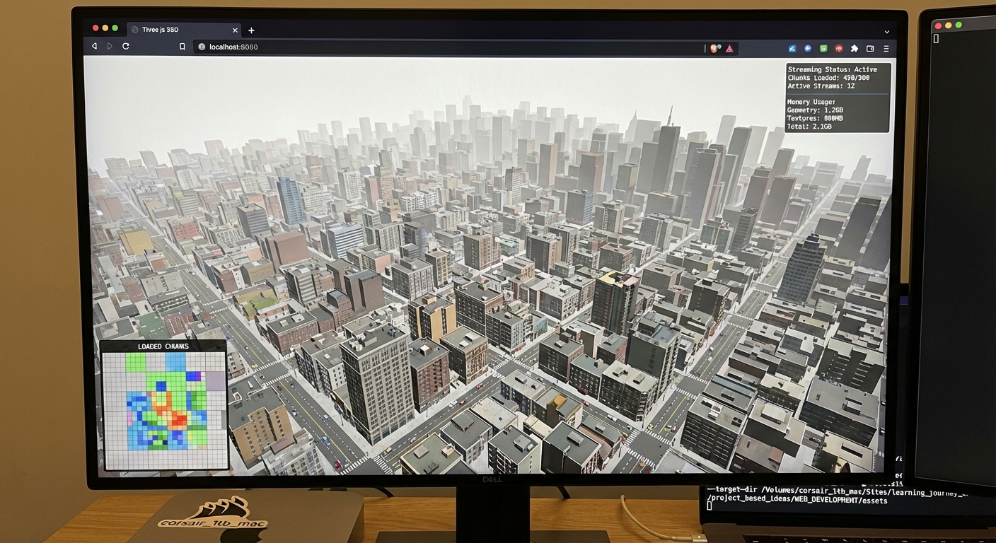
The Core Question You Are Answering
“How do you stream large worlds continuously while keeping frame time and memory stable?”
This matters because teams fail less from missing features and more from systems that cannot be reasoned about under change. This project trains you to design for predictability, instrumentation, and controlled growth.
Concepts You Must Understand First
- Deterministic Update Order
- Which systems run first, and what state do they own?
- Book Reference: “Game Engine Architecture” streaming and resource chapters
- Resource Lifecycle Management
- When is data loaded, retained, and evicted?
- Book Reference: “Game Engine Architecture” by Jason Gregory - resource chapters
- Event and Message Boundaries
- Which events are domain events versus UI-only events?
- Book Reference: “Game Programming Patterns” by Robert Nystrom - event queue chapter
- Profiling and Telemetry
- Which metrics prove correctness and performance?
- Book Reference: “Real-Time Rendering” by Akenine-Moller - optimization chapters
Questions to Guide Your Design
- Which state is authoritative, and which state is a derived view?
- What is your fixed-step versus variable-step policy?
- How will you prove subsystem isolation during a failure test?
- What are your frame-time and memory budgets for this project?
- How will you detect regression automatically after adding a new feature?
Thinking Exercise
Exercise: Failure Budget Tabletop
Create a table with three scenarios: latency spike, memory spike, and event storm. For each scenario, trace the exact subsystem boundary where the issue should be contained, the metric that detects it first, and the expected recovery strategy.
Questions to answer:
- Which invariant breaks first in each scenario?
- Which recovery action is safe during the current frame?
- Which signals prove the system returned to healthy state?
The Interview Questions They Will Ask
- “How did you decide system boundaries in this project?”
- “Which metrics did you track to prove the architecture works?”
- “How do you reproduce and debug a non-deterministic bug in real time systems?”
- “What tradeoffs did you make between abstraction and performance?”
- “How would this design evolve if user count or world size doubled?”
Hints in Layers
Hint 1: Start with contracts, not features Write a one-page runtime contract defining ownership, ordering, and lifecycle before implementation.
Hint 2: Instrument early Add telemetry from day one so regressions are visible while the system is still small.
Hint 3: Add controlled failure injection Introduce toggles that simulate delays or dropped events to validate resilience.
Hint 4: Validate with repeatable scripts Use a deterministic scenario playback to compare metrics before and after each change.
Books That Will Help
| Topic | Book | Chapter |
|---|---|---|
| Runtime design | “Game Engine Architecture” streaming and resource chapters | Relevant architecture chapters |
| Performance diagnostics | “Real-Time Rendering” by Akenine-Moller | Pipeline optimization chapters |
| System boundaries | “Game Programming Patterns” by Robert Nystrom | Update, event queue, state |
Common Pitfalls and Debugging
Problem 1: “Behavior differs between runs”
- Why: Update ordering or hidden mutable state is non-deterministic.
- Fix: Enforce deterministic ordering and isolate mutable ownership.
- Quick test: Replay the same deterministic input stream twice and diff telemetry output.
Problem 2: “Performance fixes break correctness”
- Why: Optimizations bypassed invariant checks.
- Fix: Keep invariants explicit and validate them after each optimization pass.
- Quick test: Run correctness assertions with optimization toggles on and off.
Problem 3: “Memory keeps growing”
- Why: Resource eviction policies are missing or too conservative.
- Fix: Add lifecycle states and eviction thresholds tied to scene scope.
- Quick test: Run a long session, capture memory high-water marks, and verify plateau behavior.
Definition of Done
- Core functionality demonstrates Large-Scale World Streaming and Memory Control in a realistic scenario
- Deterministic replay script produces stable outcomes
- Telemetry panel exposes frame, memory, and subsystem timings
- At least one controlled failure injection path is implemented and documented
- Recovery path succeeds without full application restart
- Performance budget stays within documented limits on reference hardware
- Architecture and invariants are documented in a short design note
Project 27: Build NPC Navigation with Navmesh, A*, and Behavior Trees
- File: P27-ai-navmesh-npc-system.md
- Main Programming Language: TypeScript
- Alternative Programming Languages: JavaScript, Rust (WASM), C# (Unity prototype parity)
- Coolness Level: 5 - Legendary
- Business Potential: 4 - Strong product fit
- Difficulty: Advanced
- Knowledge Area: AI Systems
- Software or Tool: Navmesh tools + Three.js + ECS AI systems
- Main Book: “Artificial Intelligence for Games” by Ian Millington
What you will build: A production-style module centered on AI and Navigation Systems for NPC Behavior with observable runtime output and measurable correctness signals.
Why it teaches Three.js: It forces you to treat Three.js as a systems runtime, not just a rendering library, by implementing Navmesh generation, path planning, local steering, obstacle avoidance, behavior trees, and perception events.
Core challenges you will face:
- Boundary design under pressure -> You must keep modules isolated while features grow.
- Runtime correctness verification -> You need explicit invariants and failure tests.
- Performance and operability tradeoffs -> Every abstraction choice affects frame time and memory.
Real World Outcome
When you open the project, you see a functional scenario proving the concept end-to-end, not a toy placeholder. The UI includes a diagnostics panel with frame time, subsystem timings, memory usage, and critical state transitions. Interactions are observable: toggling a subsystem shows measurable impact, failure injection demonstrates recovery behavior, and logs annotate the exact phase where work happened. The project includes a repeatable walkthrough document so a reviewer can run the same sequence and confirm identical outcomes. By the end, you can demonstrate stable behavior under normal load, controlled degradation under stress, and a clear explanation of why the architecture holds.
Observable session transcript (example):
action: boot project result: all subsystem health checks green action: run stress preset result: frame time rises from 11.4ms to 15.8ms, no dropped simulation ticks action: enable debug overlays result: timing histogram and queue depth visible in HUD action: trigger recovery test result: degraded subsystem is isolated and recovers without full restart
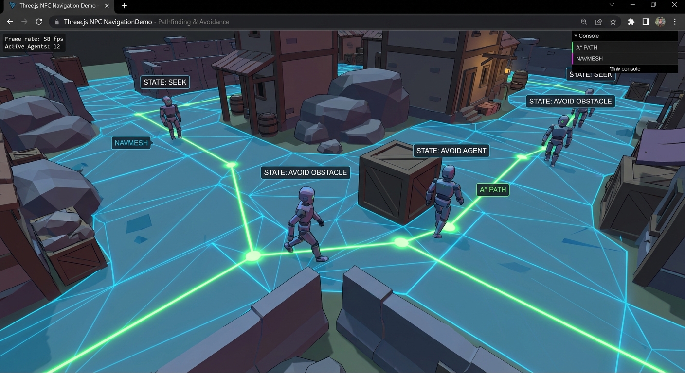
The Core Question You Are Answering
“How do you move many NPCs believably through dynamic spaces without scripted rails?”
This matters because teams fail less from missing features and more from systems that cannot be reasoned about under change. This project trains you to design for predictability, instrumentation, and controlled growth.
Concepts You Must Understand First
- Deterministic Update Order
- Which systems run first, and what state do they own?
- Book Reference: “Artificial Intelligence for Games” by Ian Millington
- Resource Lifecycle Management
- When is data loaded, retained, and evicted?
- Book Reference: “Game Engine Architecture” by Jason Gregory - resource chapters
- Event and Message Boundaries
- Which events are domain events versus UI-only events?
- Book Reference: “Game Programming Patterns” by Robert Nystrom - event queue chapter
- Profiling and Telemetry
- Which metrics prove correctness and performance?
- Book Reference: “Real-Time Rendering” by Akenine-Moller - optimization chapters
Questions to Guide Your Design
- Which state is authoritative, and which state is a derived view?
- What is your fixed-step versus variable-step policy?
- How will you prove subsystem isolation during a failure test?
- What are your frame-time and memory budgets for this project?
- How will you detect regression automatically after adding a new feature?
Thinking Exercise
Exercise: Failure Budget Tabletop
Create a table with three scenarios: latency spike, memory spike, and event storm. For each scenario, trace the exact subsystem boundary where the issue should be contained, the metric that detects it first, and the expected recovery strategy.
Questions to answer:
- Which invariant breaks first in each scenario?
- Which recovery action is safe during the current frame?
- Which signals prove the system returned to healthy state?
The Interview Questions They Will Ask
- “How did you decide system boundaries in this project?”
- “Which metrics did you track to prove the architecture works?”
- “How do you reproduce and debug a non-deterministic bug in real time systems?”
- “What tradeoffs did you make between abstraction and performance?”
- “How would this design evolve if user count or world size doubled?”
Hints in Layers
Hint 1: Start with contracts, not features Write a one-page runtime contract defining ownership, ordering, and lifecycle before implementation.
Hint 2: Instrument early Add telemetry from day one so regressions are visible while the system is still small.
Hint 3: Add controlled failure injection Introduce toggles that simulate delays or dropped events to validate resilience.
Hint 4: Validate with repeatable scripts Use a deterministic scenario playback to compare metrics before and after each change.
Books That Will Help
| Topic | Book | Chapter |
|---|---|---|
| Runtime design | “Artificial Intelligence for Games” by Ian Millington | Relevant architecture chapters |
| Performance diagnostics | “Real-Time Rendering” by Akenine-Moller | Pipeline optimization chapters |
| System boundaries | “Game Programming Patterns” by Robert Nystrom | Update, event queue, state |
Common Pitfalls and Debugging
Problem 1: “Behavior differs between runs”
- Why: Update ordering or hidden mutable state is non-deterministic.
- Fix: Enforce deterministic ordering and isolate mutable ownership.
- Quick test: Replay the same deterministic input stream twice and diff telemetry output.
Problem 2: “Performance fixes break correctness”
- Why: Optimizations bypassed invariant checks.
- Fix: Keep invariants explicit and validate them after each optimization pass.
- Quick test: Run correctness assertions with optimization toggles on and off.
Problem 3: “Memory keeps growing”
- Why: Resource eviction policies are missing or too conservative.
- Fix: Add lifecycle states and eviction thresholds tied to scene scope.
- Quick test: Run a long session, capture memory high-water marks, and verify plateau behavior.
Definition of Done
- Core functionality demonstrates AI and Navigation Systems for NPC Behavior in a realistic scenario
- Deterministic replay script produces stable outcomes
- Telemetry panel exposes frame, memory, and subsystem timings
- At least one controlled failure injection path is implemented and documented
- Recovery path succeeds without full application restart
- Performance budget stays within documented limits on reference hardware
- Architecture and invariants are documented in a short design note
Project 28: Recreate a Simplified PBR Rendering Pipeline
- File: P28-engine-level-pbr-pipeline.md
- Main Programming Language: TypeScript
- Alternative Programming Languages: JavaScript, Rust (WASM), C# (Unity prototype parity)
- Coolness Level: 5 - Legendary
- Business Potential: 4 - Strong product fit
- Difficulty: Expert
- Knowledge Area: Advanced Rendering
- Software or Tool: GLSL + Three.js custom materials
- Main Book: “Physically Based Rendering” and RTR shading chapters
What you will build: A production-style module centered on Engine-Level Rendering: BRDF and Tone Mapping with observable runtime output and measurable correctness signals.
Why it teaches Three.js: It forces you to treat Three.js as a systems runtime, not just a rendering library, by implementing Cook-Torrance BRDF terms, linear workflow, shadow filtering, tone mapping operators, and validation captures against reference renders.
Core challenges you will face:
- Boundary design under pressure -> You must keep modules isolated while features grow.
- Runtime correctness verification -> You need explicit invariants and failure tests.
- Performance and operability tradeoffs -> Every abstraction choice affects frame time and memory.
Real World Outcome
When you open the project, you see a functional scenario proving the concept end-to-end, not a toy placeholder. The UI includes a diagnostics panel with frame time, subsystem timings, memory usage, and critical state transitions. Interactions are observable: toggling a subsystem shows measurable impact, failure injection demonstrates recovery behavior, and logs annotate the exact phase where work happened. The project includes a repeatable walkthrough document so a reviewer can run the same sequence and confirm identical outcomes. By the end, you can demonstrate stable behavior under normal load, controlled degradation under stress, and a clear explanation of why the architecture holds.
Observable session transcript (example):
action: boot project result: all subsystem health checks green action: run stress preset result: frame time rises from 11.4ms to 15.8ms, no dropped simulation ticks action: enable debug overlays result: timing histogram and queue depth visible in HUD action: trigger recovery test result: degraded subsystem is isolated and recovers without full restart
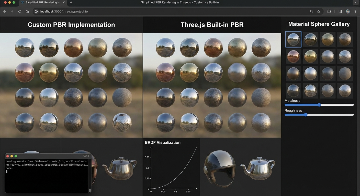
The Core Question You Are Answering
“How do you reason about physically based rendering quality instead of tweaking sliders blindly?”
This matters because teams fail less from missing features and more from systems that cannot be reasoned about under change. This project trains you to design for predictability, instrumentation, and controlled growth.
Concepts You Must Understand First
- Deterministic Update Order
- Which systems run first, and what state do they own?
- Book Reference: “Physically Based Rendering” and RTR shading chapters
- Resource Lifecycle Management
- When is data loaded, retained, and evicted?
- Book Reference: “Game Engine Architecture” by Jason Gregory - resource chapters
- Event and Message Boundaries
- Which events are domain events versus UI-only events?
- Book Reference: “Game Programming Patterns” by Robert Nystrom - event queue chapter
- Profiling and Telemetry
- Which metrics prove correctness and performance?
- Book Reference: “Real-Time Rendering” by Akenine-Moller - optimization chapters
Questions to Guide Your Design
- Which state is authoritative, and which state is a derived view?
- What is your fixed-step versus variable-step policy?
- How will you prove subsystem isolation during a failure test?
- What are your frame-time and memory budgets for this project?
- How will you detect regression automatically after adding a new feature?
Thinking Exercise
Exercise: Failure Budget Tabletop
Create a table with three scenarios: latency spike, memory spike, and event storm. For each scenario, trace the exact subsystem boundary where the issue should be contained, the metric that detects it first, and the expected recovery strategy.
Questions to answer:
- Which invariant breaks first in each scenario?
- Which recovery action is safe during the current frame?
- Which signals prove the system returned to healthy state?
The Interview Questions They Will Ask
- “How did you decide system boundaries in this project?”
- “Which metrics did you track to prove the architecture works?”
- “How do you reproduce and debug a non-deterministic bug in real time systems?”
- “What tradeoffs did you make between abstraction and performance?”
- “How would this design evolve if user count or world size doubled?”
Hints in Layers
Hint 1: Start with contracts, not features Write a one-page runtime contract defining ownership, ordering, and lifecycle before implementation.
Hint 2: Instrument early Add telemetry from day one so regressions are visible while the system is still small.
Hint 3: Add controlled failure injection Introduce toggles that simulate delays or dropped events to validate resilience.
Hint 4: Validate with repeatable scripts Use a deterministic scenario playback to compare metrics before and after each change.
Books That Will Help
| Topic | Book | Chapter |
|---|---|---|
| Runtime design | “Physically Based Rendering” and RTR shading chapters | Relevant architecture chapters |
| Performance diagnostics | “Real-Time Rendering” by Akenine-Moller | Pipeline optimization chapters |
| System boundaries | “Game Programming Patterns” by Robert Nystrom | Update, event queue, state |
Common Pitfalls and Debugging
Problem 1: “Behavior differs between runs”
- Why: Update ordering or hidden mutable state is non-deterministic.
- Fix: Enforce deterministic ordering and isolate mutable ownership.
- Quick test: Replay the same deterministic input stream twice and diff telemetry output.
Problem 2: “Performance fixes break correctness”
- Why: Optimizations bypassed invariant checks.
- Fix: Keep invariants explicit and validate them after each optimization pass.
- Quick test: Run correctness assertions with optimization toggles on and off.
Problem 3: “Memory keeps growing”
- Why: Resource eviction policies are missing or too conservative.
- Fix: Add lifecycle states and eviction thresholds tied to scene scope.
- Quick test: Run a long session, capture memory high-water marks, and verify plateau behavior.
Definition of Done
- Core functionality demonstrates Engine-Level Rendering: BRDF and Tone Mapping in a realistic scenario
- Deterministic replay script produces stable outcomes
- Telemetry panel exposes frame, memory, and subsystem timings
- At least one controlled failure injection path is implemented and documented
- Recovery path succeeds without full application restart
- Performance budget stays within documented limits on reference hardware
- Architecture and invariants are documented in a short design note
Project Comparison Table
| Project | Difficulty | Time | Depth of Understanding | Fun Factor |
|---|---|---|---|---|
| 1. The Spinning Cube | Beginner | Weekend | Foundation - scene graph, renderer, animation loop | ★★★☆☆ |
| 2. Solar System Mobile | Intermediate | Weekend | Medium - hierarchical transforms, orbital math | ★★★★☆ |
| 3. Textured Earth and Moon | Intermediate | Weekend | Medium - texture mapping, UV coordinates, lighting models | ★★★★☆ |
| 4. Interactive Museum | Intermediate | 1-2 weeks | High - raycasting, event systems, camera controls | ★★★★★ |
| 5. GLTF Model Viewer | Intermediate | Weekend | Medium - asset pipeline, model loading, animations | ★★★★☆ |
| 6. Physics-Based Playground | Advanced | 2-3 weeks | Very High - physics engines, collision detection, constraints | ★★★★★ |
| 7. Custom Shader Water | Expert | 2-3 weeks | Expert - GLSL, shader pipeline, GPU programming | ★★★★★ |
| 8. Post-Processing Effects Gallery | Intermediate | 1 week | High - render targets, multi-pass rendering, compositing | ★★★★☆ |
| 9. Procedural Terrain Generator | Advanced | 2-3 weeks | Very High - noise functions, LOD, GPU-driven geometry | ★★★★★ |
| 10. First-Person 3D Environment | Advanced | 2-3 weeks | Very High - spatial indexing, collision, input systems | ★★★★★ |
| 11. Particle System Showcase | Advanced | 2-3 weeks | Very High - GPU particles, instancing, shader math | ★★★★★ |
| 12. 3D Data Visualization Dashboard | Intermediate | 1-2 weeks | High - data mapping, interaction design, 3D UI | ★★★☆☆ |
| 13. Responsive 3D Portfolio Website | Advanced | 2-3 weeks | High - scroll animation, responsive 3D, performance | ★★★★☆ |
| 14. Build a Mini Game Engine Architecture | Expert | 2-4 weeks | Expert - runtime architecture, ECS boundaries, operability | ★★★★★ |
| 15. Build a Third-Person Character Controller with Animation Blending | Expert | 2-4 weeks | Expert - locomotion state graphs and animation blending | ★★★★★ |
| 16. Build a Multiplayer Web Arena Game | Expert | 2-4 weeks | Expert - replication, prediction, and lag compensation | ★★★★★ |
| 17. Build a Destructible Physics Sandbox | Expert | 2-4 weeks | Expert - advanced collision and constraint stability | ★★★★★ |
| 18. Generate an Infinite Terrain World | Expert | 2-4 weeks | Expert - procedural streaming and memory discipline | ★★★★★ |
| 19. Build a Stylized Shader Lab (Toon, Water, Fire) | Expert | 2-4 weeks | Expert - shader architecture and stylized lighting models | ★★★★★ |
| 20. Build a Post-Processing Engine without EffectComposer | Expert | 2-4 weeks | Expert - pass graphs, HDR pipeline, SSAO internals | ★★★★★ |
| 21. Optimize a Heavy Scene to 60 FPS on Mobile | Advanced | 2-4 weeks | Expert - profiling workflow and adaptive quality systems | ★★★★★ |
| 22. Build a WebXR VR Room with Hand and AR Interaction | Expert | 2-4 weeks | Expert - XR session lifecycle and comfort constraints | ★★★★★ |
| 23. Build a Full Asset Pipeline from Blender to Three.js | Advanced | 2-4 weeks | Expert - DCC-to-runtime content reliability and scale | ★★★★★ |
| 24. Implement a Dynamic Day/Night Lighting System | Expert | 2-4 weeks | Expert - IBL calibration, shadows, volumetric continuity | ★★★★★ |
| 25. Build an In-World UI + HUD Integration System | Advanced | 2-4 weeks | Expert - spatial UX patterns and input routing | ★★★★★ |
| 26. Create a Dynamically Streamed 3D City | Expert | 2-4 weeks | Expert - partitioning, async streaming, memory unloading | ★★★★★ |
| 27. Build NPC Navigation with Navmesh, A*, and Behavior Trees | Advanced | 2-4 weeks | Expert - navigation, steering, decision systems | ★★★★★ |
| 28. Recreate a Simplified PBR Rendering Pipeline | Expert | 2-4 weeks | Expert - BRDF theory and renderer-level validation | ★★★★★ |
Recommendation
If you are new to 3D graphics: Start with Project 1 (The Spinning Cube). It strips away every distraction and forces you to understand the three pillars – scene, camera, renderer – plus the animation loop. Every subsequent project assumes you have internalized this foundation. Move sequentially through Projects 2 and 3 to build your understanding of transforms, textures, and lighting before tackling anything interactive.
If you are a web developer looking to add 3D to your skillset: Start with Project 1 to establish the fundamentals, then jump directly to Project 5 (GLTF Model Viewer). The GLTF workflow is what you will use in production – loading assets created by designers, displaying them in browsers, and optimizing for performance. From there, move to Project 13 (Responsive 3D Portfolio Website) to see how Three.js integrates with real web layouts, scroll events, and responsive design patterns you already know.
If you want to build games: Follow the path Project 1 -> Project 2 -> Project 4 -> Project 6 -> Project 10. This progression builds from basic scene management through interactive raycasting, physics simulation, and finally a complete first-person environment with collision detection and spatial partitioning. Project 6 teaches you how physics engines couple with the render loop, and Project 10 puts everything together into a navigable world.
If you want creative and artistic work: Focus on Projects 7, 8, 9, and 11. These are where the visual magic lives. Project 7 teaches you to write custom shaders from scratch – the single most powerful skill for creating unique visuals. Project 8 shows you how post-processing transforms ordinary scenes into cinematic experiences. Project 9 generates infinite landscapes procedurally, and Project 11 gives you GPU-driven particle systems for effects that would be impossible on the CPU.
If you want to build your portfolio and career: Focus on Projects 5, 12, and 13. Project 5 demonstrates you can work with production asset pipelines (GLTF is the industry standard). Project 12 shows you can apply 3D to business problems – data visualization dashboards are a growing niche where Three.js developers command premium rates. Project 13 ties everything into a portfolio piece that demonstrates both technical skill and design sensibility.
If you want true engine-level mastery: Continue with Projects 14-28 in order. That sequence adds architecture, networking, procedural streaming, XR, AI navigation, and rendering internals so your Three.js knowledge scales beyond visual demos into production engineering.
Final Overall Project: The Immersive 3D Experience
The Goal: Combine Projects 5, 6, 8, 10, and 11 into a single first-person explorable environment that showcases every major Three.js subsystem working together.
You will build an immersive 3D world where a user navigates in first person through an environment populated with GLTF models, physics-interactive objects, particle effects, and post-processing passes. The experience includes ambient audio visualization, a HUD with a minimap, and seamless transitions between indoor and outdoor spaces.
Architecture Overview
+------------------------------------------------------------------+
|                    MAIN APPLICATION LOOP                          |
|                                                                   |
|  +------------------+  +------------------+  +-----------------+  |
|  |  INPUT MANAGER   |  |  PHYSICS ENGINE  |  |  AUDIO ANALYZER |  |
|  |  keyboard/mouse  |  |  Cannon/Rapier   |  |  Web Audio API  |  |
|  |  pointer lock    |  |  collision world  |  |  FFT data       |  |
|  +--------+---------+  +--------+---------+  +--------+--------+  |
|           |                      |                     |          |
|           v                      v                     v          |
|  +------------------+  +------------------+  +-----------------+  |
|  |  PLAYER CONTROL  |  |  SCENE MANAGER   |  |  PARTICLE SYS   |  |
|  |  FPS controller  |  |  GLTF loader     |  |  GPU instanced  |  |
|  |  collision resp.  |  |  LOD switching   |  |  audio-reactive |  |
|  +--------+---------+  +--------+---------+  +--------+--------+  |
|           |                      |                     |          |
|           +----------+-----------+----------+----------+          |
|                      |                      |                     |
|                      v                      v                     |
|           +------------------+   +-------------------+            |
|           |   SCENE GRAPH    |   |   POST-PROCESSING |            |
|           |   render queue   |   |   bloom, DOF, fog |            |
|           |   frustum cull   |   |   color grading   |            |
|           +--------+---------+   +--------+----------+            |
|                    |                       |                      |
|                    v                       v                      |
|           +-------------------------------------------+           |
|           |           WebGL RENDERER                  |           |
|           |           + HUD overlay (minimap)         |           |
|           +-------------------------------------------+           |
+------------------------------------------------------------------+
Step 1: World Structure and Navigation Build the first-person controller from Project 10 with pointer lock, WASD movement, and gravity. Create a ground plane and bounding walls. Implement a spatial grid for collision queries. The player should be able to walk, jump, and look around smoothly at 60 FPS.
Step 2: GLTF Asset Population Using the loader pipeline from Project 5, load multiple GLTF models into the scene – furniture, architectural elements, decorative objects. Place them with physics colliders from Project 6 so the player cannot walk through them. Implement LOD switching for distant objects to maintain frame rate.
Step 3: Physics Interaction Add throwable and pushable objects using the physics system from Project 6. The player should be able to pick up objects with a raycast (click to grab, click to release), and thrown objects should bounce and collide realistically with the environment and other objects.
Step 4: Particle Effects Integrate the GPU particle system from Project 11. Add ambient particles (dust motes, fireflies, embers) that react to the player’s movement. Create localized effects – a fountain, a torch with sparks, a portal with swirling energy. Connect at least one particle emitter to an audio analyzer so it pulses with ambient music.
Step 5: Post-Processing Pipeline Apply the multi-pass post-processing chain from Project 8. Include bloom for bright light sources, depth-of-field for cinematic focus, fog for atmosphere, and a subtle film grain pass. Make the post-processing parameters shift based on the player’s location – entering a dark cave increases bloom sensitivity and adds chromatic aberration.
Step 6: Audio Visualization Connect the Web Audio API to analyze a background music track in real-time. Feed FFT frequency data into the particle systems and into a custom shader that makes certain surfaces pulse with the beat. The audio should be spatialized so volume changes with distance from the source.
Step 7: HUD and Minimap Render a second orthographic camera view into a small viewport in the corner showing a top-down minimap. Display the player’s position and heading as an arrow. Mark interactive objects and points of interest on the minimap. Add a crosshair, FPS counter, and interaction prompts to the HUD.
Step 8: Performance Optimization Profile the complete experience. Implement frustum culling, object pooling for particles, texture atlasing for repeated materials, and draw call batching. Target a consistent 60 FPS on a mid-range GPU. Add a quality settings menu that adjusts shadow resolution, particle count, and post-processing complexity.
Success Criteria:
- The experience loads within 5 seconds on a broadband connection
- First-person navigation feels smooth with no perceptible input lag
- At least 5 distinct GLTF models are placed in the environment
- Physics objects respond correctly to player interaction and to each other
- Particle effects run at full frame rate with at least 10,000 visible particles
- Post-processing adapts to scene context (indoor vs outdoor, dark vs bright)
- Audio visualization is visibly synced to the music with less than 50ms latency
- Minimap accurately reflects the player’s position and orientation in real-time
- The entire experience runs at 60 FPS on a machine with a GTX 1060 or equivalent
- The project is deployable as a static site with no server-side dependencies
From Learning to Production: What Is Next
| Your Project | Production Equivalent | Gap to Fill |
|---|---|---|
| 1. The Spinning Cube | Product 3D previews (Apple, Nike configurators) | Asset pipeline, e-commerce integration, accessibility |
| 2. Solar System Mobile | Educational 3D simulations (NASA Eyes, Celestia) | Real orbital data ingestion, time controls, scientific accuracy |
| 3. Textured Earth and Moon | Google Earth-style globes, Mapbox GL | Tile-based texture streaming, geospatial projections, massive datasets |
| 4. Interactive Museum | Virtual showrooms (IKEA Place, Matterport) | Room scanning, AR placement, measurement tools |
| 5. GLTF Model Viewer | Sketchfab, Adobe Dimension, model-viewer web component | Annotation systems, embed APIs, format conversion pipelines |
| 6. Physics-Based Playground | Browser-based games (Krunker.io, HexGL) | Networked multiplayer, anti-cheat, server-authoritative physics |
| 7. Custom Shader Water | Shader editors (Shadertoy, ISF Editor) | Shader graph UIs, real-time parameter tweaking, cross-platform GLSL |
| 8. Post-Processing Effects Gallery | Unreal Engine post-process volumes, Unity URP | Temporal anti-aliasing, motion vectors, HDR tone mapping pipelines |
| 9. Procedural Terrain Generator | Open-world game engines, Google Earth terrain | Streaming LOD (CDLOD/CLOD), vegetation systems, biome simulation |
| 10. First-Person 3D Environment | Walkthrough tools (Enscape, Twinmotion) | BIM integration, VR headset support, multi-user sessions |
| 11. Particle System Showcase | VFX tools (Niagara, PopcornFX) | Node-based particle editors, GPU compute shaders, volumetric effects |
| 12. 3D Data Visualization Dashboard | Kepler.gl, Deck.gl, Bloomberg Terminal 3D views | Real-time data streaming, WebSocket feeds, accessibility compliance |
| 13. Responsive 3D Portfolio Website | Award-winning sites (Awwwards, FWA winners) | CMS integration, SEO for 3D content, progressive enhancement |
| 14. Build a Mini Game Engine Architecture | Production subsystem aligned with Mini Game Engine Architecture for Three.js | Hardening, observability, and scale testing |
| 15. Build a Third-Person Character Controller with Animation Blending | Production subsystem aligned with Advanced Animation System and Character Controllers | Hardening, observability, and scale testing |
| 16. Build a Multiplayer Web Arena Game | Production subsystem aligned with Real-Time Multiplayer Architecture on the Web | Hardening, observability, and scale testing |
| 17. Build a Destructible Physics Sandbox | Production subsystem aligned with Advanced Physics and Collision Systems | Hardening, observability, and scale testing |
| 18. Generate an Infinite Terrain World | Production subsystem aligned with Procedural World Generation at Scale | Hardening, observability, and scale testing |
| 19. Build a Stylized Shader Lab (Toon, Water, Fire) | Production subsystem aligned with Custom Shader Mastery and Stylized Rendering | Hardening, observability, and scale testing |
| 20. Build a Post-Processing Engine without EffectComposer | Production subsystem aligned with Post-Processing Pipeline Engineering | Hardening, observability, and scale testing |
| 21. Optimize a Heavy Scene to 60 FPS on Mobile | Production subsystem aligned with Performance Engineering for Mobile 60 FPS | Hardening, observability, and scale testing |
| 22. Build a WebXR VR Room with Hand and AR Interaction | Production subsystem aligned with WebXR VR and AR Systems | Hardening, observability, and scale testing |
| 23. Build a Full Asset Pipeline from Blender to Three.js | Production subsystem aligned with Production Asset Pipeline: Blender to Runtime | Hardening, observability, and scale testing |
| 24. Implement a Dynamic Day/Night Lighting System | Production subsystem aligned with Advanced Lighting and Time-of-Day Systems | Hardening, observability, and scale testing |
| 25. Build an In-World UI + HUD Integration System | Production subsystem aligned with 3D UI Architecture and Interaction Design | Hardening, observability, and scale testing |
| 26. Create a Dynamically Streamed 3D City | Production subsystem aligned with Large-Scale World Streaming and Memory Control | Hardening, observability, and scale testing |
| 27. Build NPC Navigation with Navmesh, A*, and Behavior Trees | Production subsystem aligned with AI and Navigation Systems for NPC Behavior | Hardening, observability, and scale testing |
| 28. Recreate a Simplified PBR Rendering Pipeline | Production subsystem aligned with Engine-Level Rendering: BRDF and Tone Mapping | Hardening, observability, and scale testing |
Summary
This learning path covers Three.js and WebGL 3D graphics programming through 28 hands-on projects that progress from fundamental scene setup to production-grade immersive experiences.
This updated edition extends the sprint with 15 additional advanced projects (Projects 14-28) that cover engine architecture, multiplayer networking, advanced physics, procedural streaming, shader pipelines, XR, asset pipelines, UI integration, AI navigation, and engine-level rendering.
| # | Project Name | Main Language | Difficulty | Time Estimate | |—|————–|—————|————|—————| | 1 | The Spinning Cube | JavaScript | Beginner | Weekend | | 2 | Solar System Mobile | JavaScript | Intermediate | Weekend | | 3 | Textured Earth and Moon | JavaScript | Intermediate | Weekend | | 4 | Interactive Museum | JavaScript | Intermediate | 1-2 weeks | | 5 | GLTF Model Viewer | JavaScript | Intermediate | Weekend | | 6 | Physics-Based Playground | JavaScript | Advanced | 2-3 weeks | | 7 | Custom Shader Water | JavaScript + GLSL | Expert | 2-3 weeks | | 8 | Post-Processing Effects Gallery | JavaScript | Intermediate | 1 week | | 9 | Procedural Terrain Generator | JavaScript + GLSL | Advanced | 2-3 weeks | | 10 | First-Person 3D Environment | JavaScript | Advanced | 2-3 weeks | | 11 | Particle System Showcase | JavaScript + GLSL | Advanced | 2-3 weeks | | 12 | 3D Data Visualization Dashboard | JavaScript | Intermediate | 1-2 weeks | | 13 | Responsive 3D Portfolio Website | JavaScript | Advanced | 2-3 weeks | | 14 | Build a Mini Game Engine Architecture | TypeScript | Expert | 2-4 weeks | | 15 | Build a Third-Person Character Controller with Animation Blending | TypeScript | Expert | 2-4 weeks | | 16 | Build a Multiplayer Web Arena Game | TypeScript | Expert | 2-4 weeks | | 17 | Build a Destructible Physics Sandbox | TypeScript | Expert | 2-4 weeks | | 18 | Generate an Infinite Terrain World | TypeScript | Expert | 2-4 weeks | | 19 | Build a Stylized Shader Lab (Toon, Water, Fire) | TypeScript | Expert | 2-4 weeks | | 20 | Build a Post-Processing Engine without EffectComposer | TypeScript | Expert | 2-4 weeks | | 21 | Optimize a Heavy Scene to 60 FPS on Mobile | TypeScript | Advanced | 2-4 weeks | | 22 | Build a WebXR VR Room with Hand and AR Interaction | TypeScript | Expert | 2-4 weeks | | 23 | Build a Full Asset Pipeline from Blender to Three.js | TypeScript | Advanced | 2-4 weeks | | 24 | Implement a Dynamic Day/Night Lighting System | TypeScript | Expert | 2-4 weeks | | 25 | Build an In-World UI + HUD Integration System | TypeScript | Advanced | 2-4 weeks | | 26 | Create a Dynamically Streamed 3D City | TypeScript | Expert | 2-4 weeks | | 27 | Build NPC Navigation with Navmesh, A*, and Behavior Trees | TypeScript | Advanced | 2-4 weeks | | 28 | Recreate a Simplified PBR Rendering Pipeline | TypeScript | Expert | 2-4 weeks | Expected Outcomes
After completing this sprint, you will be able to:
- Build complete 3D applications from scratch using Three.js without relying on boilerplate or starter templates
- Understand the WebGL rendering pipeline from JavaScript API calls through vertex shaders to fragment output
- Write custom GLSL shaders for water, terrain, particles, and post-processing effects
- Integrate physics engines with the render loop for realistic object interaction
- Load, display, and optimize GLTF models following production asset pipeline practices
- Implement first-person navigation with collision detection and spatial partitioning
- Build GPU-instanced particle systems that handle tens of thousands of particles at 60 FPS
- Apply multi-pass post-processing chains including bloom, depth-of-field, and color grading
- Generate procedural geometry and terrain using noise functions and LOD techniques
- Profile and optimize 3D web applications for consistent frame rates on mid-range hardware
- Create responsive 3D experiences that adapt to different screen sizes and device capabilities
- Map 3D visualization techniques to real-world data for dashboards and analytical tools
Additional Resources and References
Standards and Specifications
- WebGL 2.0 Specification - The underlying graphics API that Three.js abstracts. Understanding WebGL helps you debug shader issues and optimize draw calls.
- GLTF 2.0 Specification - The 3D asset format used in Projects 5 and the Final Project. Read the materials and animation sections carefully.
- GLSL ES 3.0 Specification - The shading language reference for Projects 7, 9, and 11. Keep this open while writing shaders.
- Web Audio API Specification - Required for the audio visualization in the Final Project.
Tools
- Blender - Free 3D modeling, texturing, and animation tool. Essential for creating and exporting GLTF assets for Projects 5, 10, and the Final Project.
- Spline - Browser-based 3D design tool with Three.js export. Useful for rapid prototyping of scenes in Projects 4 and 13.
- lil-gui - Lightweight GUI for tweaking parameters in real time. Indispensable during shader development in Projects 7, 8, and 9.
- Stats.js - FPS and memory monitor by the Three.js creator. Use in every project for performance awareness.
- Spector.js - WebGL debugging tool that captures and inspects draw calls, shader state, and textures. Critical for debugging Projects 7-11.
- glTF Validator - Validates GLTF files against the specification. Use before loading models in Project 5.
- Shader Editor (browser extension) - Live-edit shaders in running WebGL applications. Accelerates iteration in Projects 7, 9, and 11.
Communities
- Three.js Discord - The most active community for real-time help. Channels organized by topic (shaders, physics, performance).
- Three.js Forum (Discourse) - Searchable archive of solutions. Many core contributors answer questions here.
- r/threejs (Reddit) - Community showcases and discussions. Good for seeing what others are building and getting feedback on your projects.
- WebGL/WebGPU Meetups - Khronos Group organizes events about the underlying standards.
Courses and Tutorials
- Three.js Journey by Bruno Simon - The most comprehensive Three.js course available. Covers nearly every topic in this guide with video walkthroughs. Particularly relevant for Projects 7 (shaders), 9 (procedural generation), and 11 (particles).
- Discover Three.js by Lewy Blue - Free online book that teaches Three.js from first principles. Excellent companion for Projects 1-5.
- The Book of Shaders by Patricio Gonzalez Vivo - Interactive introduction to GLSL. Essential reading before attempting Projects 7, 9, and 11.
- WebGL Fundamentals - If you want to understand what Three.js does under the hood. Read after completing Project 1 to deepen your understanding of the rendering pipeline.
Books
- “Real-Time Rendering, 4th Edition” by Tomas Akenine-Moller et al. - Ch. 5 (Shading Basics), Ch. 6 (Texturing), Ch. 14 (Acceleration Structures). The definitive reference for understanding the graphics pipeline that underlies Three.js.
- “Fundamentals of Computer Graphics, 5th Edition” by Steve Marschner and Peter Shirley - Ch. 4 (Ray Tracing), Ch. 7 (Viewing), Ch. 8 (The Graphics Pipeline). Strong mathematical foundation for 3D transformations used in every project.
- “WebGL Programming Guide” by Kouichi Matsuda and Rodger Lea - Ch. 5 (Colors and Textures), Ch. 8 (Lighting), Ch. 10 (Advanced Techniques). Bridges the gap between Three.js abstractions and raw WebGL.
- “Mathematics for 3D Game Programming and Computer Graphics, 3rd Edition” by Eric Lengyel - Ch. 4 (Transforms), Ch. 5 (Geometry), Ch. 8 (Visibility). The math reference you need for Projects 6, 9, and 10.
- “GPU Gems” series (NVIDIA) - Available free online. Ch. 1 (Water Rendering) directly applies to Project 7. Ch. 38 (Fast Fluid Dynamics) applies to Project 11.
- “The Nature of Code” by Daniel Shiffman - Ch. 4 (Particle Systems), Ch. 6 (Autonomous Agents). Conceptual foundation for Project 11, with code examples easily adapted to Three.js.
- “Interactive Computer Graphics, 8th Edition” by Edward Angel and Dave Shreiner - Ch. 3 (Geometric Objects), Ch. 5 (Lighting and Shading), Ch. 9 (Procedural Methods). Academic foundation for the theory primer concepts applied in Projects 3, 7, and 9.