Learn The Art of Computer Programming: From Zero to Knuth Master

Goal: Build a working, internal model of TAOCP that goes beyond reading proofs. You will implement the core algorithms, data structures, and mathematical tools Knuth relies on, then validate them with empirical experiments and careful analysis. By the end, you will be able to translate TAOCP’s MIX/MMIX-style descriptions into real, correct, and efficient code, reason about performance with rigorous asymptotics, and explain why each algorithm works. The projects are sequenced to mirror the volumes: foundations first, then data structures, randomization, arithmetic, sorting/searching, and combinatorial methods.

Why TAOCP Matters

“The Art of Computer Programming” is widely considered the most comprehensive and rigorous work on computer science ever written. Bill Gates famously said, “If you think you’re a really good programmer… read Knuth’s Art of Computer Programming… You should definitely send me a résumé if you can read the whole thing.”

TAOCP teaches you to:

Think mathematically about algorithms—analyzing their efficiency precisely
Understand computers at the deepest level—from machine instructions to abstract algorithms
Develop problem-solving skills that separate great programmers from good ones
Master fundamental techniques that underpin all of computer science

The Practical Why

TAOCP is not a book of trivia. It is a machine for building transferable mental models:

When a system slows down, you can reason about whether the cause is algorithmic growth, data structure shape, or memory layout.
When you need a random generator, you will know how to test it rather than trust it.
When you implement a search structure, you will know the exact invariants that keep it fast.
When you compare algorithms, you will be able to quantify why one wins in practice.

This matters because real systems are built from these primitives. Databases depend on B-trees. Compilers depend on trees and symbol tables. Security depends on precise arithmetic and bit manipulation. Performance depends on choosing the right algorithm for the input distribution. TAOCP is the source code for all of that.

After completing these projects, you will:

Understand algorithm analysis using Knuth’s rigorous mathematical framework
Be able to implement any data structure from first principles
Know the theory behind random number generation and can test for randomness
Master every major sorting and searching algorithm with their trade-offs
Solve hard combinatorial problems using backtracking and SAT solvers
Have implemented a working RISC computer (MMIX) to truly understand machines

The Big Picture: From Math to Machine

TAOCP is a single story told at multiple layers. The projects are designed to make that story visible:

Mathematics ──► Algorithms ──► Data Structures ──► Machine Model ──► Performance
     |               |                |                |               |
  proofs         procedures        invariants       MMIX code        analysis

If you can move left to right in this pipeline, you can turn a theorem into working code. If you can move right to left, you can explain why a program behaves the way it does. This is the core skill TAOCP builds.

How the projects map to the pipeline:

Math Toolkit + Randomness build the proof and analysis layer.
Data Structures + Trees + Sorting build the invariants and algorithm layer.
MMIX + Arithmetic build the machine model layer.
Combinatorics + SAT build the search and optimization layer.

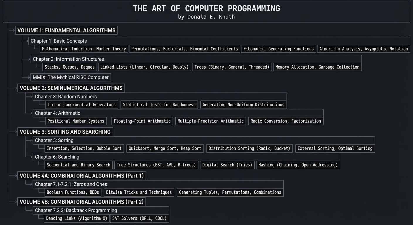
TAOCP Volume Overview

┌─────────────────────────────────────────────────────────────────────────────┐
│                    THE ART OF COMPUTER PROGRAMMING                          │
│                         by Donald E. Knuth                                  │
├─────────────────────────────────────────────────────────────────────────────┤
│                                                                             │
│  VOLUME 1: FUNDAMENTAL ALGORITHMS                                          │
│  ├── Chapter 1: Basic Concepts                                             │
│  │   ├── Mathematical Induction, Number Theory                             │
│  │   ├── Permutations, Factorials, Binomial Coefficients                   │
│  │   ├── Fibonacci, Generating Functions                                   │
│  │   └── Algorithm Analysis, Asymptotic Notation                           │
│  ├── Chapter 2: Information Structures                                     │
│  │   ├── Stacks, Queues, Deques                                            │
│  │   ├── Linked Lists (Linear, Circular, Doubly)                           │
│  │   ├── Trees (Binary, General, Threaded)                                 │
│  │   └── Memory Allocation, Garbage Collection                             │
│  └── MMIX: The Mythical RISC Computer                                      │
│                                                                             │
│  VOLUME 2: SEMINUMERICAL ALGORITHMS                                        │
│  ├── Chapter 3: Random Numbers                                             │
│  │   ├── Linear Congruential Generators                                    │
│  │   ├── Statistical Tests for Randomness                                  │
│  │   └── Generating Non-Uniform Distributions                              │
│  └── Chapter 4: Arithmetic                                                 │
│      ├── Positional Number Systems                                         │
│      ├── Floating-Point Arithmetic                                         │
│      ├── Multiple-Precision Arithmetic                                     │
│      └── Radix Conversion, Factorization                                   │
│                                                                             │
│  VOLUME 3: SORTING AND SEARCHING                                           │
│  ├── Chapter 5: Sorting                                                    │
│  │   ├── Insertion, Selection, Bubble Sort                                 │
│  │   ├── Quicksort, Merge Sort, Heap Sort                                  │
│  │   ├── Distribution Sorting (Radix, Bucket)                              │
│  │   └── External Sorting, Optimal Sorting                                 │
│  └── Chapter 6: Searching                                                  │
│      ├── Sequential and Binary Search                                      │
│      ├── Tree Structures (BST, AVL, B-trees)                               │
│      ├── Digital Search (Tries)                                            │
│      └── Hashing (Chaining, Open Addressing)                               │
│                                                                             │
│  VOLUME 4A: COMBINATORIAL ALGORITHMS (Part 1)                              │
│  └── Chapter 7.1-7.2.1: Zeros and Ones                                     │
│      ├── Boolean Functions, BDDs                                           │
│      ├── Bitwise Tricks and Techniques                                     │
│      └── Generating Tuples, Permutations, Combinations                     │
│                                                                             │
│  VOLUME 4B: COMBINATORIAL ALGORITHMS (Part 2)                              │
│  └── Chapter 7.2.2: Backtrack Programming                                  │
│      ├── Dancing Links (Algorithm X)                                       │
│      └── SAT Solvers (DPLL, CDCL)                                          │
│                                                                             │
└─────────────────────────────────────────────────────────────────────────────┘

taocp volume overview

Knuth’s Exercise Difficulty Scale

TAOCP uses a unique rating system for exercises (0-50):

Rating	Meaning
00	Immediate—you should see the answer instantly
10	Simple—a minute of thought should suffice
20	Medium—may take 15-20 minutes
30	Moderately hard—requires significant work
40	Quite difficult—term paper level
50	Research problem—unsolved or PhD-level
M	Mathematical—requires math beyond calculus
HM	Higher mathematics—graduate level math

Our projects target concepts from exercises rated 10-40, making TAOCP accessible through practical implementation.

Prerequisites & Background Knowledge

Essential Prerequisites (Must Have)

C programming fundamentals: pointers, structs, manual memory management, and file I/O.
Discrete math basics: induction, summations, permutations/combinations, and modular arithmetic.
Comfort with proofs: you should be able to follow a proof, even if you do not write them daily.
Algorithm literacy: Big-O notation and basic data structures (arrays, linked lists, trees).

Helpful But Not Required

Assembly exposure: even a short introduction helps when reading MMIX.
Probability & statistics: useful for randomness and testing distributions.
Numerical methods: helpful for Chapter 4 (arithmetic and precision).

Self-Assessment Questions

Can you implement a linked list without memory leaks?
Can you explain the difference between O(n log n) and O(n^2)?
Can you follow a proof by induction and re-derive a result with small examples?
Can you compute factorials, binomial coefficients, and Fibonacci numbers without a calculator?

Development Environment Setup

Compiler: gcc or clang with -Wall -Wextra -Werror
Build: make (use Makefiles for repeatable experiments)
Plotting (optional): Python + matplotlib for performance charts
Testing: a lightweight test harness (e.g., a tests/ directory + a single runner)

Time Investment

Foundations: 2-4 weeks
MMIX + data structures: 4-6 weeks
Random numbers + arithmetic: 3-5 weeks
Sorting/searching + combinatorics: 4-8 weeks

Important Reality Check

TAOCP is rigorous by design. Expect to revisit chapters multiple times. Your reward is a durable, machine-level understanding that transfers to any language or system you build later.

Core Concept Analysis

Think of TAOCP as six interlocking concept clusters. Each project reinforces one cluster while depending on the previous ones.

A. Mathematical Foundations and Analysis

Central question: How do you prove that an algorithm is correct and quantify its cost?

Key ideas:

Asymptotic notation (O, Ω, Θ) and rigorous bounding
Summations and recurrences for time analysis
Generating functions to solve recurrence relations
Induction as the default proof technique

What this unlocks:

You can predict performance before writing code.
You can explain why a slow algorithm fails at scale.
You can justify correctness beyond “it seems to work.”

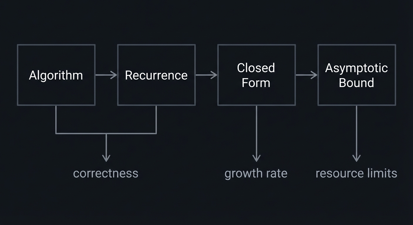
Algorithm → Recurrence → Closed Form → Asymptotic Bound
   │              │             │             │
   │              ▼             ▼             ▼
   └────────── correctness   growth rate   resource limits

taocp analysis pipeline

B. Information Structures and Memory

Central question: How do you represent data so operations are fast and predictable?

Key ideas:

Stacks, queues, deques as fundamental building blocks
Linked structures and pointer invariants
Trees (binary, general, threaded) and traversal mechanics
Storage allocation and garbage collection strategies

What this unlocks:

You can reason about memory usage and locality.
You can build robust, leak-free data structures.
You can choose the right structure for the workload.

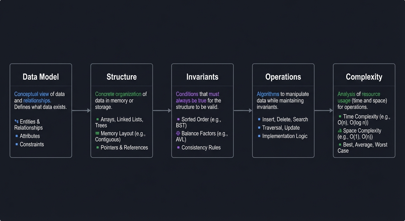
Data Model ──► Structure ──► Invariants ──► Operations ──► Complexity

taocp data structure pipeline

C. Randomness and Experimental Validation

Central question: How do we generate randomness and validate its properties?

Key ideas:

Linear congruential generators and period analysis
Statistical tests (frequency, runs, serial correlation)
Transforming distributions (uniform → non-uniform)

What this unlocks:

You can test RNG quality instead of trusting it.
You can build simulations and sampling pipelines confidently.

D. Arithmetic and Precision

Central question: How does the machine represent numbers and where does error creep in?

Key ideas:

Radix representation and mixed-radix systems
Multiple-precision arithmetic and carry propagation
Floating-point error and rounding analysis

What this unlocks:

You can build reliable numeric code.
You can spot precision bugs and edge cases.

E. Sorting and Searching as Systems

Central question: Why do these algorithms actually behave the way the analysis predicts?

Key ideas:

Distribution vs comparison sorting
Tree-based searching and balancing
Hashing and collision behavior

What this unlocks:

You can select algorithms based on data distribution, not habit.
You can quantify when a data structure stops scaling.

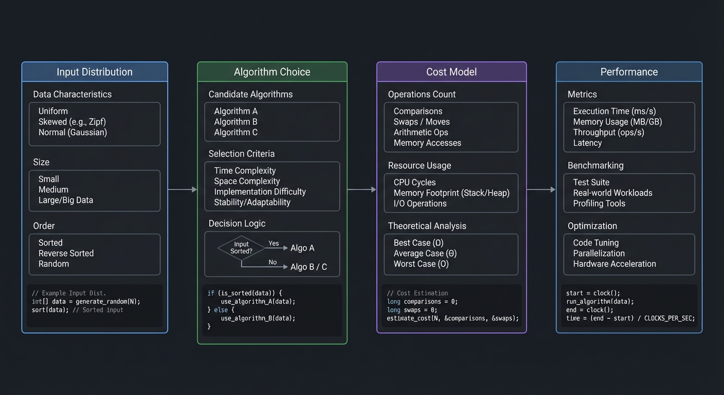
Input Distribution ──► Algorithm Choice ──► Cost Model ──► Performance

taocp performance model pipeline

F. Combinatorial Algorithms and Backtracking

Central question: How do you explore enormous search spaces efficiently?

Key ideas:

Generating tuples/permutations/combinations
Algorithm X and Dancing Links
SAT solving strategies (DPLL/CDCL)

What this unlocks:

You can model and solve constraint problems (Sudoku, scheduling, verification).
You can build practical search tools with strong pruning.

Success Metrics (What “Mastery” Looks Like)

You can consider this track successful when you can:

Explain any algorithm in TAOCP in plain language and derive its complexity.
Implement the algorithm from scratch without external libraries.
Test correctness with invariant checks and small exhaustive inputs.
Predict performance trends as input size grows.
Translate TAOCP’s MMIX descriptions into working code.

These are the same skills used in high-end systems, database, and compiler work.

How to Use This Guide

If you want to finish these projects, follow this workflow for each one:

Read the Core Question and restate it in your own words.
Skim the Concepts and look up any missing definitions immediately.
Do the Thinking Exercise on paper first (it makes the code obvious).
Implement in small layers and verify each layer with tests.
Compare results to theory using the provided formulas or counts.

Golden rule: every project should end with both correctness proof and empirical validation. If you cannot validate, you do not yet understand it.

Definitions & Notation You Must Be Fluent In

O(g(n)): upper bound on growth rate (worst-case ceiling).
Ω(g(n)): lower bound (best-case floor).
Θ(g(n)): tight bound (both upper and lower).
[x] / ⌊x⌋ / ⌈x⌉: floor/ceiling operators.
Σ / Π: summation and product notation used constantly in TAOCP.
Invariant: a property that must remain true after every operation.
Algorithm (Knuth’s sense): a finite sequence of precise, effective steps.

Concept Summary Table

Concept Cluster	What You Need to Internalize
Mathematical Foundations	Translate algorithms into recurrences, solve them, and justify bounds.
Information Structures	Maintain pointer invariants and reason about storage costs.
Randomness & Tests	Generate random sequences and detect non-randomness with statistical checks.
Arithmetic & Precision	Implement number representations and quantify rounding error.
Sorting & Searching	Choose algorithms based on input distribution and cost models.
Combinatorial Methods	Generate and search large state spaces without brute-force explosion.
MMIX & Machine Model	Map abstract algorithms to a concrete machine and instruction set.

Deep Dive Reading by Concept

Concept	Primary TAOCP Source	Supporting Book
Mathematical analysis	Volume 1, Ch. 1	Concrete Mathematics Ch. 1-3
Data structures	Volume 1, Ch. 2	Algorithms in C Parts 1-4
Random numbers	Volume 2, Ch. 3	Algorithms in C Part 4 (Random)
Arithmetic	Volume 2, Ch. 4	Computer Systems: A Programmer’s Perspective Ch. 2
Sorting/searching	Volume 3, Ch. 5-6	Algorithms, 4th Edition Ch. 2-3
Combinatorial algorithms	Volume 4A/4B, Ch. 7	The Recursive Book of Recursion Ch. 7-9
Machine model (MMIX)	Volume 1, Fascicle 1	Write Great Code, Vol. 1 Ch. 3

Quick Start (First 48 Hours)

Read TAOCP Vol. 1, Ch. 1 overview and skim the notation section.
Implement a small math toolkit: factorial, binomial coefficients, and Fibonacci (iterative + fast).
Write a tiny benchmarking harness to compare naive vs optimized approaches.
Prove one lemma (e.g., sum of first n integers) with induction in your own words.
Create a notes file that tracks definitions and symbols you encounter.

Recommended Learning Paths

Path A: Systems-first (if you like hardware)

Project 1 (MMIX Simulator)
Project 2 (Mathematical Toolkit)
Projects on data structures and memory
Sorting/searching projects

Path B: Math-first (if you like proofs)

Project 2 (Mathematical Toolkit)
Randomness + arithmetic projects
Data structure projects
MMIX simulator last

Path C: Interview/Industry-first

Sorting and searching projects
Data structures projects
Randomness and testing
Combinatorial algorithms

Project List

Projects are organized by TAOCP volume and chapter, building from foundations to advanced topics.

VOLUME 1: FUNDAMENTAL ALGORITHMS

Project 1: MMIX Simulator (Understand the Machine)

File: LEARN_TAOCP_DEEP_DIVE.md
Main Programming Language: C
Alternative Programming Languages: Rust, C++, Go
Coolness Level: Level 5: Pure Magic
Business Potential: 1. The “Resume Gold”
Difficulty: Level 4: Expert
Knowledge Area: Computer Architecture / Assembly / Emulation
Software or Tool: Building: CPU Emulator
Main Book: “The Art of Computer Programming, Volume 1, Fascicle 1: MMIX” by Donald E. Knuth

What you’ll build: A complete simulator for MMIX, Knuth’s 64-bit RISC computer architecture, capable of running MMIX assembly programs with full instruction set support.

Why it teaches TAOCP: All algorithms in TAOCP are presented in MMIX assembly language. To truly understand the book, you need to understand the machine. Building an MMIX simulator teaches you computer architecture from the ground up—registers, memory, instruction encoding, and execution.

Core challenges you’ll face:

Implementing 256 general-purpose registers → maps to register file design
Decoding 256 instruction opcodes → maps to instruction set architecture
Simulating memory with virtual addressing → maps to memory hierarchy
Implementing special registers (rA, rD, etc.) → maps to processor state

Key Concepts:

MMIX Architecture: “TAOCP Volume 1, Fascicle 1” - Donald E. Knuth
Computer Organization: “Computer Organization and Design RISC-V Edition” Chapter 2 - Patterson & Hennessy
Instruction Encoding: “The MMIX Supplement” - Martin Ruckert
CPU Simulation: “Write Great Code, Volume 1” Chapter 3 - Randall Hyde

Resources for key challenges:

Knuth’s MMIX Page - Official documentation
GIMMIX Simulator - Reference implementation

Difficulty: Expert Time estimate: 3-4 weeks Prerequisites:

Basic C programming
Understanding of binary/hexadecimal
Willingness to read Knuth’s MMIX specification

Real world outcome:

$ cat hello.mms
        LOC   #100
Main    GETA  $255,String
        TRAP  0,Fputs,StdOut
        TRAP  0,Halt,0
String  BYTE  "Hello, MMIX World!",#a,0

$ ./mmixal hello.mms     # Assemble
$ ./mmix hello.mmo       # Run
Hello, MMIX World!

$ ./mmix -t hello.mmo    # Trace execution
1. 0000000000000100: e7ff0010 (GETA) $255 = #0000000000000110
2. 0000000000000104: 00000601 (TRAP) Fputs to StdOut
   Hello, MMIX World!
3. 0000000000000108: 00000000 (TRAP) Halt

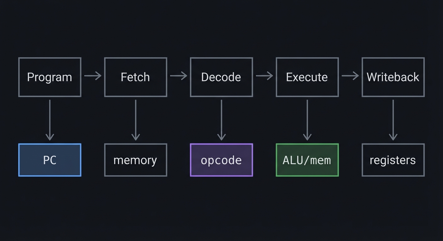
Visual Model

Program -> Fetch -> Decode -> Execute -> Writeback
   |         |         |         |           |
  PC      memory     opcode    ALU/mem     registers

taocp fetch decode execute

The Core Question You’re Answering

“How does a concrete machine execute an algorithm step by step, and how do its rules shape every TAOCP program?”

Concepts You Must Understand First

Instruction encoding and field extraction (TAOCP Vol 1, Fascicle 1)
Register files and program counter discipline
Addressing modes, alignment, and byte order
Traps, interrupts, and privileged behavior
State invariants (what must remain true after every step)

Questions to Guide Your Design

How will you represent memory so byte, wyde, tetra, and octa accesses are correct?
What is your instruction decode strategy (table, switch, or data-driven)?
How do you model special registers and side effects cleanly?
How will you test correctness for each opcode without writing 256 bespoke tests?

Thinking Exercise

Hand-execute this microprogram by tracking registers and PC:

SETL $1,#0001
SETL $2,#0002
ADD  $3,$1,$2
STOU $3,0($0)

What value ends up at address 0? What is PC after the last instruction?

The Interview Questions They’ll Ask

How do you decode and dispatch instructions efficiently?
What is the difference between a trap and an interrupt?
How would you validate emulator correctness?
What are the classic endianness pitfalls?

Hints in Layers

Hint 1: Start Small Implement just memory, registers, PC, and a handful of opcodes (ADD, LDOU, STOU).

Hint 2: Build a Tiny Assembler Loader Parse a minimal subset of MMIXAL output to avoid full assembler complexity.

Hint 3: Add Traps as Function Hooks Map TRAP instructions to host callbacks for I/O.

Hint 4: Create a Golden Trace Use known instruction traces and compare register snapshots after each step.

Books That Will Help

Topic	Book	Chapter
MMIX execution	TAOCP Vol 1, Fascicle 1	Entire fascicle
CPU organization	Computer Organization and Design	Ch. 2-3
Emulator structure	Write Great Code, Vol. 1	Ch. 3
Low-level execution	Low-Level Programming	Ch. 1-2

Common Pitfalls & Debugging

Problem: “Registers look correct but memory is wrong”

Why: Endianness or misaligned access in loads/stores.
Fix: Verify byte ordering with a known pattern (0x0102030405060708).
Quick test: Store a constant, then load it byte-by-byte and compare.

Problem: “PC jumps unpredictably”

Why: Forgetting to increment PC for non-branch instructions.
Fix: Centralize PC increment and only override for branch/trap.
Quick test: Run a straight-line program and verify PC progression by 4.

Implementation Hints:

MMIX register structure:

General registers: $0 - $255 (64-bit each)
Special registers:
  rA - Arithmetic status
  rB - Bootstrap register
  rC - Continuation register
  rD - Dividend register
  rE - Epsilon register
  rH - Himult register
  rJ - Return-jump register
  rM - Multiplex mask
  rR - Remainder register
  rBB, rTT, rWW, rXX, rYY, rZZ - Trip registers

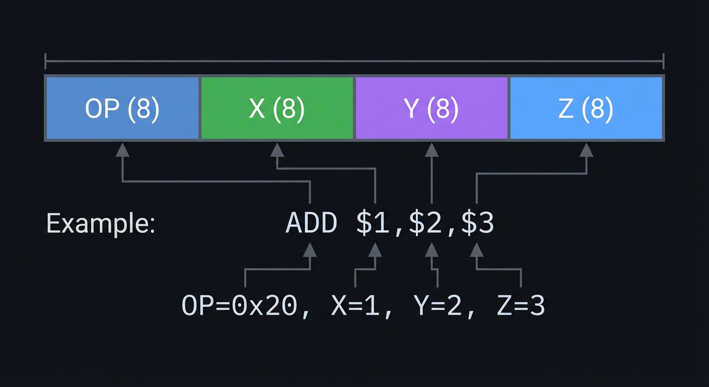
Instruction format (32 bits):

┌────────┬────────┬────────┬────────┐
│ OP (8) │ X (8)  │ Y (8)  │ Z (8)  │
└────────┴────────┴────────┴────────┘
Example: ADD $1,$2,$3
  OP=0x20, X=1, Y=2, Z=3

taocp instruction format

Core execution loop:

while (!halted) {
    instruction = memory[PC];
    OP = (instruction >> 24) & 0xFF;
    X = (instruction >> 16) & 0xFF;
    Y = (instruction >> 8) & 0xFF;
    Z = instruction & 0xFF;

    switch (OP) {
        case 0x20: // ADD
            reg[X] = reg[Y] + reg[Z];
            break;
        case 0xF8: // POP (return)
            // Complex stack unwinding
            break;
        // ... 254 more cases
    }
    PC += 4;
}

Think about:

How do you handle overflow in arithmetic operations?
What happens on TRAP instructions (system calls)?
How do you implement the stack with rO and rS?
How do you handle interrupts and trips?

Learning milestones:

Basic arithmetic instructions work → You understand ALU operations
Memory loads/stores work → You understand addressing modes
Branches and jumps work → You understand control flow
TRAP instructions work → You understand I/O and system calls
Can run TAOCP example programs → You’re ready for the algorithms!

Definition of Done

Runs the sample MMIX program and produces correct output
Opcode test suite covers arithmetic, load/store, branch, and TRAP
Trace output matches a golden trace for a known program
Memory and register invariants validated after each step

Project 2: Mathematical Toolkit (TAOCP’s Foundations)

File: LEARN_TAOCP_DEEP_DIVE.md
Main Programming Language: C
Alternative Programming Languages: Rust, Python, Haskell
Coolness Level: Level 3: Genuinely Clever
Business Potential: 1. The “Resume Gold”
Difficulty: Level 2: Intermediate
Knowledge Area: Mathematics / Number Theory / Combinatorics
Software or Tool: Building: Math Library
Main Book: “The Art of Computer Programming, Volume 1” Chapter 1 - Knuth

What you’ll build: A comprehensive mathematical library implementing the foundations from TAOCP Chapter 1—including arbitrary precision arithmetic, binomial coefficients, Fibonacci numbers, harmonic numbers, and generating functions.

Why it teaches TAOCP: Chapter 1 is the mathematical foundation for everything that follows. Knuth uses these tools constantly—binomial coefficients for counting, generating functions for solving recurrences, and harmonic numbers for algorithm analysis.

Core challenges you’ll face:

Implementing binomial coefficients without overflow → maps to Pascal’s triangle
Computing Fibonacci numbers efficiently → maps to matrix exponentiation
Harmonic number approximations → maps to asymptotic analysis
Polynomial arithmetic → maps to generating functions

Key Concepts:

Mathematical Induction: TAOCP Vol 1, Section 1.2.1
Binomial Coefficients: TAOCP Vol 1, Section 1.2.6
Fibonacci Numbers: TAOCP Vol 1, Section 1.2.8
Generating Functions: TAOCP Vol 1, Section 1.2.9
Asymptotic Notation: TAOCP Vol 1, Section 1.2.11

Difficulty: Intermediate Time estimate: 1-2 weeks Prerequisites:

Basic algebra and calculus
C programming with arbitrary precision (or implement it)
Interest in mathematics

Real world outcome:

$ ./math_toolkit

math> binomial 100 50
100891344545564193334812497256

math> fibonacci 1000
43466557686937456435688527675040625802564660517371780402481729089536555417949051890403879840079255169295922593080322634775209689623239873322471161642996440906533187938298969649928516003704476137795166849228875

math> harmonic 1000000
14.392726722865723631415730

math> gcd 1234567890 987654321
9

math> solve_recurrence "F(n) = F(n-1) + F(n-2), F(0)=0, F(1)=1"
Closed form: F(n) = (phi^n - psi^n) / sqrt(5)
Where phi = (1+sqrt(5))/2, psi = (1-sqrt(5))/2

math> prime_factorize 1234567890
2 × 3² × 5 × 3607 × 3803

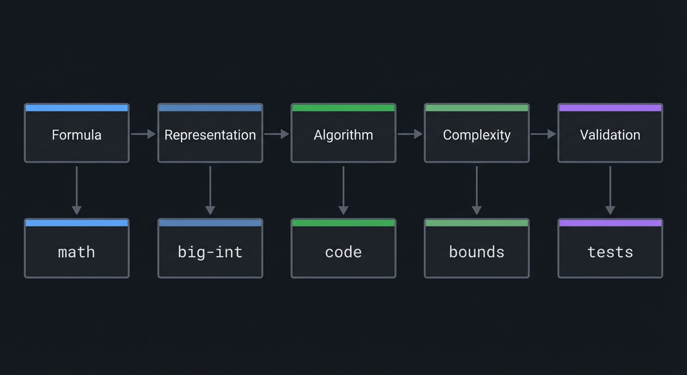
Visual Model

Formula -> Representation -> Algorithm -> Complexity -> Validation
   |            |              |            |            |
  math        big-int         code        bounds      tests

taocp math toolkit pipeline

The Core Question You’re Answering

“How do you compute and analyze mathematical quantities exactly, without losing correctness to overflow or approximation?”

Concepts You Must Understand First

Integer representations and overflow (CS:APP Ch. 2)
Induction and recurrence solving (Concrete Mathematics Ch. 1-3)
Modular arithmetic and GCD
Generating functions and series manipulation

Questions to Guide Your Design

What base will you store digits in, and how does it impact speed?
When do you use exact formulas vs approximations?
How will you validate results for very large inputs?
Which functions need memoization to stay fast?

Thinking Exercise

Compute by hand:

C(6,3)
H(5) = 1 + 1/2 + 1/3 + 1/4 + 1/5
gcd(252, 198)

Then verify your toolkit matches each result.

The Interview Questions They’ll Ask

How do you compute Fibonacci in O(log n)?
Why does naive binomial overflow, and how do you avoid it?
How do you implement gcd efficiently?
What is a generating function and why is it useful?

Hints in Layers

Hint 1: Start With BigInt Add/Sub Everything else relies on correct carry propagation.

Hint 2: Implement gcd and modular exponent These unlock many later algorithms and tests.

Hint 3: Add Binomial and Fibonacci Use multiplicative formulas and fast doubling/matrix methods.

Hint 4: Validate With Known Sequences Compare with published values (Catalan numbers, Fibonacci, primes).

Books That Will Help

Topic	Book	Chapter
Induction and recurrences	Concrete Mathematics	Ch. 1-3
Integer representation	CS:APP	Ch. 2
Algorithmic math	Math for Programmers	Ch. 2-4
Fundamental algorithms	TAOCP Vol 1	Ch. 1

Common Pitfalls & Debugging

Problem: “Binomial results are incorrect for large n”

Why: Intermediate multiplication overflows before division.
Fix: Multiply/divide incrementally and reduce by gcd.
Quick test: Compare C(100,50) with a known value.

Problem: “Harmonic approximation is off”

Why: Using too few terms in the asymptotic expansion.
Fix: Add more terms or use direct summation for smaller n.
Quick test: Compare H(10^6) to a high-precision reference.

Implementation Hints:

Efficient binomial coefficient:

// C(n,k) = n! / (k! * (n-k)!)
// But compute incrementally to avoid overflow

uint64_t binomial(int n, int k) {
    if (k > n - k) k = n - k;  // C(n,k) = C(n, n-k)
    uint64_t result = 1;
    for (int i = 0; i < k; i++) {
        result = result * (n - i) / (i + 1);  // Order matters!
    }
    return result;
}

Fibonacci via matrix exponentiation:

[F(n+1)]   [1 1]^n   [1]
[F(n)  ] = [1 0]   × [0]

Matrix power in O(log n) using repeated squaring!

Harmonic numbers with Euler-Maclaurin:

H(n) ≈ ln(n) + γ + 1/(2n) - 1/(12n²) + 1/(120n⁴) - ...
Where γ ≈ 0.5772156649... (Euler-Mascheroni constant)

Think about:

How do you compute binomial(1000, 500) without overflow?
What’s the fastest way to compute Fibonacci(1000000)?
How do you represent generating functions as data structures?
How precise should harmonic number approximations be?

Learning milestones:

Binomials compute correctly → You understand Pascal’s triangle
Large Fibonacci numbers work → You understand matrix exponentiation
Harmonic approximations are accurate → You understand asymptotics
GCD is efficient → You understand Euclid’s algorithm

Definition of Done

Big-int add/sub/mul/div pass randomized tests
Binomial/Fibonacci/Harmonic outputs match known values
Recurrence solver matches closed forms for sample inputs
Benchmarks show asymptotically faster methods win at scale

Project 3: Dynamic Data Structures Library

File: LEARN_TAOCP_DEEP_DIVE.md
Main Programming Language: C
Alternative Programming Languages: Rust, C++
Coolness Level: Level 3: Genuinely Clever
Business Potential: 2. The “Micro-SaaS / Pro Tool”
Difficulty: Level 2: Intermediate
Knowledge Area: Data Structures / Memory Management
Software or Tool: Building: Data Structures Library
Main Book: “The Art of Computer Programming, Volume 1” Chapter 2 - Knuth

What you’ll build: A complete library of fundamental data structures as described in TAOCP Chapter 2—stacks, queues, deques, linked lists (all variants), and general trees.

Why it teaches TAOCP: Chapter 2 covers information structures—how data lives in memory. Knuth’s treatment is deeper than most textbooks, covering circular lists, doubly-linked lists, symmetric lists, and orthogonal lists. You’ll understand the design choices at the deepest level.

Core challenges you’ll face:

Implementing all linked list variants → maps to pointer manipulation
Circular doubly-linked lists → maps to symmetric structures
Tree traversals and threading → maps to recursive structures
Memory allocation and garbage collection → maps to storage management

Key Concepts:

Stacks and Queues: TAOCP Vol 1, Section 2.2.1
Linked Lists: TAOCP Vol 1, Section 2.2.3-2.2.5
Trees: TAOCP Vol 1, Sections 2.3.1-2.3.3
Garbage Collection: TAOCP Vol 1, Section 2.3.5

Difficulty: Intermediate Time estimate: 2 weeks Prerequisites:

C programming (pointers, malloc/free)
Basic data structure concepts
Project 1 helpful but not required

Real world outcome:

$ ./test_structures

Testing circular doubly-linked list:
  Insert: A -> B -> C -> D -> (back to A)
  Forward traverse: A B C D A B C ...
  Backward traverse: D C B A D C B ...
  Delete C: A -> B -> D -> (back to A)
  ✓ All operations O(1)

Testing threaded binary tree:
  Inorder: A B C D E F G
  Inorder successor of D: E (via thread, O(1))
  Inorder predecessor of D: C (via thread, O(1))
  ✓ No stack needed for traversal!

Testing garbage collection:
  Allocated 10000 nodes
  Created reference cycles
  Running mark-sweep GC...
  Freed 7500 unreachable nodes
  ✓ Memory reclaimed correctly

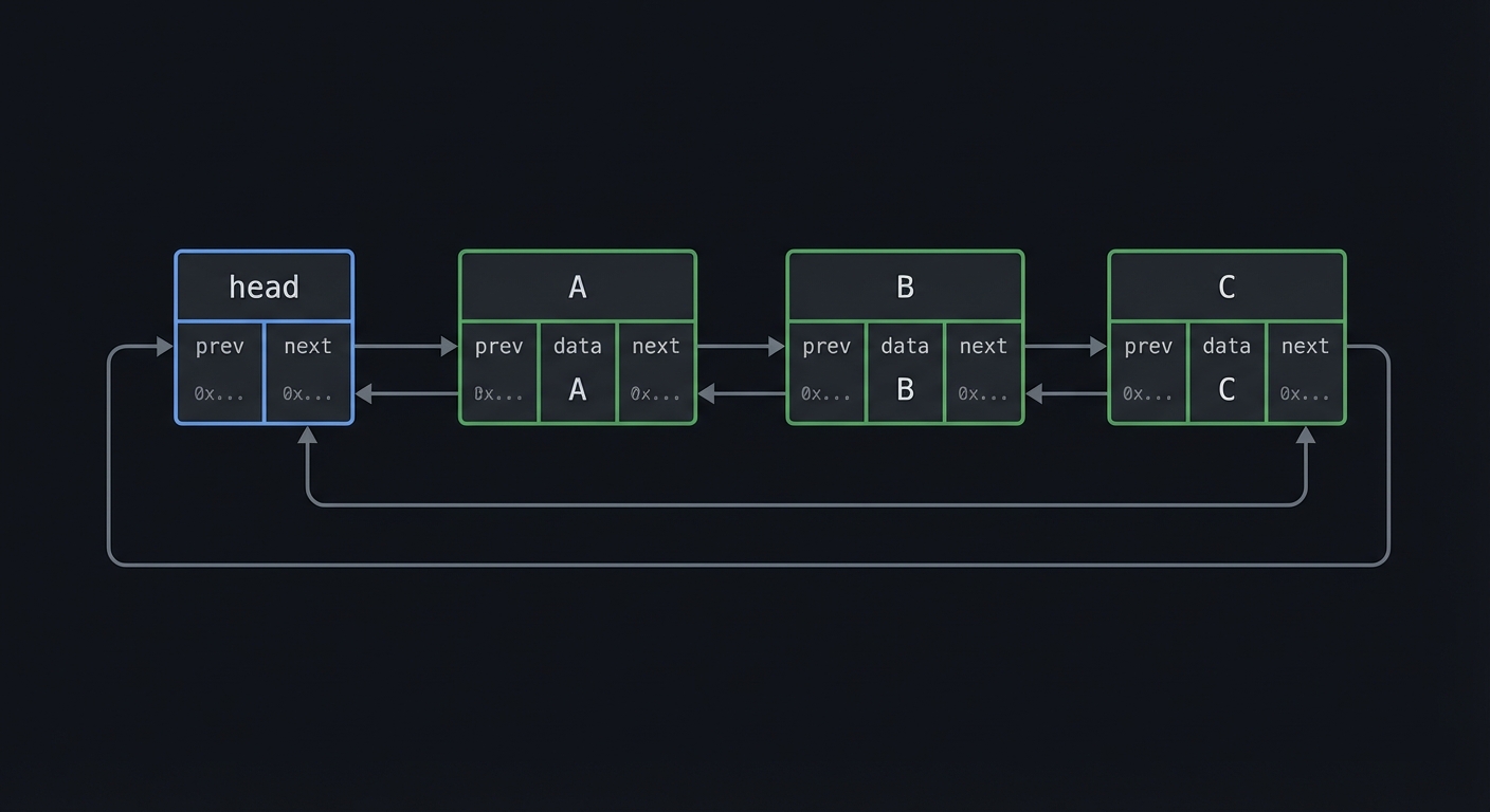
Visual Model

[head] <-> [A] <-> [B] <-> [C] <-> [head]
  ^                                      |
  +--------------------------------------+

taocp circular list

The Core Question You’re Answering

“How do you keep pointer-based structures correct under every insert, delete, and traversal?”

Concepts You Must Understand First

Pointer invariants and ownership rules
Sentinel nodes and circular list advantages
Stack/queue/deque semantics
Heap allocation strategies and GC basics

Questions to Guide Your Design

Will you use sentinels to simplify empty-list edge cases?
How will you enforce invariants after each mutation?
How will you test for memory leaks and dangling pointers?
Which operations must be O(1), and which can be O(n)?

Thinking Exercise

Draw a circular doubly-linked list with nodes A, B, C. Delete B and update the four pointer assignments by hand.

The Interview Questions They’ll Ask

Why use a circular list instead of NULL-terminated?
How do you implement a queue with O(1) enqueue/dequeue?
What are common linked-list bugs in C?
How would you detect and fix a memory leak?

Hints in Layers

Hint 1: Start With Stack and Queue These are the simplest structures and build confidence.

Hint 2: Add a Sentinel Head It removes special cases and simplifies deletion.

Hint 3: Implement Threaded Trees Separately Keep the list library small and reliable.

Hint 4: Add GC as an Independent Module Test GC with a synthetic graph of nodes and cycles.

Books That Will Help

Topic	Book	Chapter
Lists and trees	TAOCP Vol 1	Ch. 2
Practical structures	Algorithms in C	Parts 1-2
Pointer discipline	Understanding and Using C Pointers	Ch. 3-6
API design	C Interfaces and Implementations	Ch. 4-6

Common Pitfalls & Debugging

Problem: “List traversal loops forever”

Why: Circular list links not updated correctly after delete.
Fix: Validate that each node’s next/prev are consistent.
Quick test: Traverse forward/backward for 2*n steps and ensure repetition.

Problem: “Random crashes on delete”

Why: Use-after-free or double-free.
Fix: Null out pointers after free and track ownership.
Quick test: Run with address sanitizer and delete every node twice in tests.

Implementation Hints:

Circular doubly-linked list node:

typedef struct Node {
    void* data;
    struct Node* prev;
    struct Node* next;
} Node;

// Empty list: head->prev = head->next = head (self-loop)
// Insert after p: new->next = p->next; new->prev = p;
//                 p->next->prev = new; p->next = new;
// Delete p: p->prev->next = p->next; p->next->prev = p->prev;

Threaded binary tree:

typedef struct TNode {
    void* data;
    struct TNode* left;
    struct TNode* right;
    bool left_is_thread;   // true if left points to predecessor
    bool right_is_thread;  // true if right points to successor
} TNode;

// Inorder successor without stack:
TNode* successor(TNode* p) {
    if (p->right_is_thread) return p->right;
    p = p->right;
    while (!p->left_is_thread) p = p->left;
    return p;
}

Mark-sweep garbage collection:

mark_phase(root):
    if root is marked: return
    mark root
    for each pointer p in root:
        mark_phase(*p)

sweep_phase():
    for each object in heap:
        if not marked:
            free(object)
        else:
            unmark object

Think about:

What’s the advantage of circular lists over NULL-terminated?
Why use threading in trees?
How does reference counting differ from mark-sweep?
What are the trade-offs of different memory allocation strategies?

Learning milestones:

All list variants work → You understand linked structures
Threaded traversal is stackless → You understand threading
GC reclaims memory correctly → You understand reachability
Performance matches expected complexity → You can analyze structures

Definition of Done

All list/stack/queue operations pass edge-case tests
Threaded tree traversal works without recursion
GC reclaims cycles and reports accurate counts
No leaks or use-after-free under sanitizers

Project 4: Tree Algorithms and Traversals

File: LEARN_TAOCP_DEEP_DIVE.md
Main Programming Language: C
Alternative Programming Languages: Rust, Go
Coolness Level: Level 3: Genuinely Clever
Business Potential: 1. The “Resume Gold”
Difficulty: Level 3: Advanced
Knowledge Area: Trees / Recursion / Combinatorics
Software or Tool: Building: Tree Library
Main Book: “The Art of Computer Programming, Volume 1” Section 2.3 - Knuth

What you’ll build: A comprehensive tree library including binary trees, general trees, forests, and the algorithms from TAOCP—including the correspondence between forests and binary trees, tree enumeration, and path length analysis.

Why it teaches TAOCP: Knuth’s treatment of trees is extraordinarily deep, covering not just operations but the combinatorics of trees—how many trees exist with n nodes, the average path length, and the natural correspondence between forests and binary trees.

Core challenges you’ll face:

Forest-to-binary-tree conversion → maps to natural correspondence
Counting trees (Catalan numbers) → maps to combinatorics
Computing path lengths → maps to algorithm analysis
Huffman encoding → maps to optimal trees

Key Concepts:

Tree Traversals: TAOCP Vol 1, Section 2.3.1 (Algorithm T, S, etc.)
Binary Trees: TAOCP Vol 1, Section 2.3.1
Tree Enumeration: TAOCP Vol 1, Section 2.3.4.4
Huffman’s Algorithm: TAOCP Vol 1, Section 2.3.4.5
Path Length: TAOCP Vol 1, Section 2.3.4.5

Difficulty: Advanced Time estimate: 2 weeks Prerequisites:

Project 3 completed
Understanding of recursion
Basic combinatorics

Real world outcome:

$ ./tree_toolkit

# Convert forest to binary tree
tree> forest_to_binary "((A B) (C (D E)) F)"
Binary tree:
      A
     /
    B
     \
      C
     /
    D
     \
      E
       \
        F

# Count binary trees with n nodes (Catalan numbers)
tree> count_trees 10
16796 distinct binary trees with 10 nodes
(This is C(10) = C(20,10)/(10+1) = 16796)

# Compute internal/external path length
tree> path_lengths "example.tree"
Internal path length: 45
External path length: 75
Relation: E = I + 2n ✓

# Build Huffman tree
tree> huffman "AAAAABBBBCCCDDE"
Symbol frequencies: A:5, B:4, C:3, D:2, E:1
Huffman codes:
  A: 0      (1 bit)
  B: 10     (2 bits)
  C: 110    (3 bits)
  D: 1110   (4 bits)
  E: 1111   (4 bits)
Average bits per symbol: 2.07
Entropy: 2.03 bits (Huffman is near-optimal!)

Visual Model

Forest:          Binary Tree:
  A               A
 /|\             /
B C D           B
  |                E               C
                                       D
                   /
                  E

The Core Question You’re Answering

“How do different tree representations change traversal, counting, and optimal coding?”

Concepts You Must Understand First

Inorder/preorder/postorder traversal invariants
Tree enumeration and Catalan numbers
Path length definitions (internal vs external)
Huffman coding and optimal prefix trees

Questions to Guide Your Design

How will you represent general trees and forests in memory?
Can you compute path lengths without recursion?
How will you verify Catalan counts for small n?
What data structure will you use for Huffman priority queue?

Thinking Exercise

Given symbols A:5, B:4, C:3, D:2, E:1, build the Huffman tree and compute average bits per symbol.

The Interview Questions They’ll Ask

Why does E = I + 2n for binary trees?
How does forest-to-binary-tree correspondence work?
What makes Huffman coding optimal?
How do you compute the number of binary trees with n nodes?

Hints in Layers

Hint 1: Implement Basic Traversals Start with recursive traversals and validate orderings.

Hint 2: Add the Forest Conversion Use first-child/next-sibling mapping.

Hint 3: Implement Catalan via DP Verify counts for n=0..10.

Hint 4: Add Huffman With a Min-Heap Each combine step removes two smallest nodes.

Books That Will Help

Topic	Book	Chapter
Tree algorithms	TAOCP Vol 1	Ch. 2.3
Practical trees	Algorithms in C	Part 5
Recursion and trees	The Recursive Book of Recursion	Ch. 7-8
Encoding	Algorithms, 4th Edition	Ch. 5

Common Pitfalls & Debugging

Problem: “Traversal output is wrong”

Why: Left/right children swapped or incorrect base cases.
Fix: Test on a tiny tree with known traversal orders.
Quick test: For tree (A (B C)), inorder should be B A C.

Problem: “Huffman codes are not prefix-free”

Why: Tree construction step not preserving left/right leaf structure.
Fix: Verify that only leaves get codes and internal nodes do not.
Quick test: Check that no code is a prefix of any other.

Implementation Hints:

Forest to binary tree (natural correspondence):

For each node in forest:
  - First child becomes LEFT child in binary tree
  - Next sibling becomes RIGHT child in binary tree

Forest:        Binary tree:
  A              A
 /|\            /
B C D          B
  |             \
  E              C
                  \
                   D
                  /
                 E

Catalan numbers (count of binary trees):

C(n) = (2n)! / ((n+1)! * n!)
C(n) = C(n-1) * 2(2n-1) / (n+1)

C(0)=1, C(1)=1, C(2)=2, C(3)=5, C(4)=14, C(5)=42, ...

Internal/External path length:

I = sum of depths of internal nodes
E = sum of depths of external nodes (null pointers)

Theorem: E = I + 2n (where n = number of internal nodes)

This is fundamental to analyzing search trees!

Huffman’s algorithm:

1. Create leaf node for each symbol with its frequency
2. While more than one node in queue:
   a. Remove two nodes with lowest frequency
   b. Create new internal node with these as children
   c. Frequency = sum of children's frequencies
   d. Insert new node back into queue
3. Remaining node is root of Huffman tree

Learning milestones:

Traversals work correctly → You understand tree navigation
Forest conversion is reversible → You understand the correspondence
Catalan numbers match tree counts → You understand enumeration
Huffman achieves near-entropy → You understand optimal coding

Definition of Done

Forest-to-binary conversion is reversible on test trees
Catalan counts match for n=0..10
Huffman codes are prefix-free and near-entropy
Path length relation E = I + 2n verified

VOLUME 2: SEMINUMERICAL ALGORITHMS

Project 5: Random Number Generator Suite

File: LEARN_TAOCP_DEEP_DIVE.md
Main Programming Language: C
Alternative Programming Languages: Rust, Go, Python
Coolness Level: Level 4: Hardcore Tech Flex
Business Potential: 3. The “Service & Support” Model
Difficulty: Level 3: Advanced
Knowledge Area: Random Numbers / Statistics / Number Theory
Software or Tool: Building: RNG Library
Main Book: “The Art of Computer Programming, Volume 2” Chapter 3 - Knuth

What you’ll build: A complete random number generation library with linear congruential generators, parameter selection, period analysis, and statistical testing—exactly as described in TAOCP Chapter 3.

Why it teaches TAOCP: Chapter 3 is the definitive treatment of random numbers. Knuth explains not just how to generate them, but how to test if they’re “random enough.” You’ll understand why rand() in most C libraries is terrible, and how to do better.

Core challenges you’ll face:

Implementing LCG with optimal parameters → maps to number theory
Computing the period of an LCG → maps to group theory
Statistical tests (chi-square, KS) → maps to hypothesis testing
The spectral test → maps to lattice theory

Key Concepts:

Linear Congruential Method: TAOCP Vol 2, Section 3.2.1
Choice of Parameters: TAOCP Vol 2, Section 3.2.1.2-3
Statistical Tests: TAOCP Vol 2, Section 3.3.1-3.3.2
Spectral Test: TAOCP Vol 2, Section 3.3.4
Other Generators: TAOCP Vol 2, Section 3.2.2

Resources for key challenges:

Linear Congruential Generator - Wikipedia - Quick reference
Spectral Test Explanation - Columbia lecture notes

Difficulty: Advanced Time estimate: 2-3 weeks Prerequisites:

Basic number theory (modular arithmetic, GCD)
Statistics fundamentals
Project 2 (mathematical toolkit) helpful

Real world outcome:

$ ./rng_suite

# Create LCG with specific parameters
rng> lcg_create m=2147483647 a=48271 c=0
LCG created: X(n+1) = 48271 * X(n) mod 2147483647

# Analyze period
rng> analyze_period
Full period achieved: 2147483646
(m-1 because c=0, so 0 is not in sequence)

# Generate and test
rng> generate 1000000
Generated 1,000,000 random numbers

rng> test_uniformity
Chi-square test (100 bins):
  χ² = 94.7, df = 99
  p-value = 0.612
  Result: PASS (uniformly distributed)

rng> test_serial
Serial correlation test:
  r = 0.00023
  Result: PASS (independent)

rng> spectral_test
Spectral test results:
  Dimension 2: ν₂ = 0.998 (excellent)
  Dimension 3: ν₃ = 0.891 (good)
  Dimension 4: ν₄ = 0.756 (acceptable)
  Dimension 5: ν₅ = 0.623 (marginal)

# Compare with bad generator
rng> lcg_create m=256 a=5 c=1
rng> spectral_test
  Dimension 2: ν₂ = 0.312 (TERRIBLE!)
  Points lie on only 8 parallel lines!

Visual Model

X(n+1) = (a * X(n) + c) mod m
   |           |    |       |
 state     multiplier inc  modulus

The Core Question You’re Answering

“How can a deterministic generator produce sequences that behave like randomness, and how do you prove it?”

Concepts You Must Understand First

Modular arithmetic and periods
Parameter selection for full period
Statistical tests (chi-square, serial correlation)
Lattice structure and the spectral test

Questions to Guide Your Design

How will you handle overflow in a * X(n)?
Which tests will you implement first to detect obvious bias?
How large a sample do you need for stable p-values?
How will you compare two generators fairly?

Thinking Exercise

Pick m=16, a=5, c=1, seed=1. Generate the first 10 outputs and plot the pairs (x_i, x_{i+1}). What pattern do you see?

The Interview Questions They’ll Ask

Why are many standard rand() implementations poor?
What does it mean for an LCG to have full period?
How do you interpret a chi-square p-value?
What does the spectral test reveal?

Hints in Layers

Hint 1: Implement LCG Core Validate with a small modulus and compare with hand computation.

Hint 2: Add Simple Uniformity Tests Histogram counts and chi-square should be your first checks.

Hint 3: Add Serial Correlation Compute correlation between successive values.

Hint 4: Implement Spectral Test Start with 2D and 3D projections and measure line spacing.

Books That Will Help

Topic	Book	Chapter
Random numbers	TAOCP Vol 2	Ch. 3
Modular math	Concrete Mathematics	Ch. 1-2
Statistical tests	Math for Programmers	Ch. 10
Empirical analysis	Algorithms, 4th Edition	Ch. 1.4

Common Pitfalls & Debugging

Problem: “Sequence repeats too early”

Why: Parameters do not meet full-period criteria.
Fix: Verify gcd(c, m)=1 and factors of m divide (a-1).
Quick test: Track first repeat of seed and compute period.

Problem: “Chi-square always fails”

Why: Using too few samples or incorrect expected counts.
Fix: Increase n and ensure each bin has expected count >= 5.
Quick test: Test a known good generator to validate your test code.

Implementation Hints:

Linear Congruential Generator:

// X(n+1) = (a * X(n) + c) mod m
typedef struct {
    uint64_t x;  // Current state
    uint64_t a;  // Multiplier
    uint64_t c;  // Increment
    uint64_t m;  // Modulus
} LCG;

uint64_t lcg_next(LCG* rng) {
    rng->x = (rng->a * rng->x + rng->c) % rng->m;
    return rng->x;
}

Knuth’s recommended parameters:

m = 2^64 (use native overflow)
a = 6364136223846793005
c = 1442695040888963407
(These pass the spectral test well)

Period analysis:

For full period (period = m), need:
1. c and m are coprime: gcd(c, m) = 1
2. a-1 is divisible by all prime factors of m
3. If m is divisible by 4, then a-1 is divisible by 4

If c = 0 (multiplicative generator):
  Period is at most m-1
  Need m prime and a primitive root mod m

Chi-square test:

Divide [0,1) into k equal bins
Generate n random numbers
Count observations in each bin: O[i]
Expected count: E = n/k
χ² = Σ (O[i] - E)² / E
Compare with chi-square distribution (k-1 df)

Learning milestones:

LCG generates correct sequence → You understand the algorithm
Period analysis is correct → You understand number theory
Chi-square test works → You understand statistical testing
Spectral test reveals quality → You understand lattice structure

Definition of Done

LCG period matches theoretical expectations
Uniformity and serial tests pass for good parameters
Spectral test differentiates good vs bad generators
Results reproducible with fixed seeds

Project 6: Arbitrary-Precision Arithmetic

File: LEARN_TAOCP_DEEP_DIVE.md
Main Programming Language: C
Alternative Programming Languages: Rust, Assembly
Coolness Level: Level 4: Hardcore Tech Flex
Business Potential: 3. The “Service & Support” Model
Difficulty: Level 4: Expert
Knowledge Area: Arithmetic / Number Theory / Algorithms
Software or Tool: Building: BigNum Library
Main Book: “The Art of Computer Programming, Volume 2” Chapter 4 - Knuth

What you’ll build: A complete arbitrary-precision arithmetic library (like GMP but simpler) implementing addition, subtraction, multiplication (including Karatsuba), division, GCD, and modular exponentiation.

Why it teaches TAOCP: Chapter 4 is the bible of computer arithmetic. You’ll learn how computers really do math—not just integer addition, but the algorithms behind calculators, cryptography, and scientific computing.

Core challenges you’ll face:

Multiple-precision addition with carry → maps to basic arithmetic
Karatsuba multiplication → maps to divide and conquer
Long division algorithm → maps to classical algorithms
Modular exponentiation → maps to cryptographic foundations

Key Concepts:

Classical Algorithms: TAOCP Vol 2, Section 4.3.1
Karatsuba Multiplication: TAOCP Vol 2, Section 4.3.3
Division: TAOCP Vol 2, Section 4.3.1 (Algorithm D)
GCD: TAOCP Vol 2, Section 4.5.2
Modular Arithmetic: TAOCP Vol 2, Section 4.3.2

Difficulty: Expert Time estimate: 3-4 weeks Prerequisites:

Solid C programming
Understanding of binary representation
Basic number theory

Real world outcome:

$ ./bignum

bignum> set A = 12345678901234567890123456789
bignum> set B = 98765432109876543210987654321
bignum> A + B
111111111011111111101111111110

bignum> A * B
1219326311370217952261850327338667891975126429917755911761289

bignum> factorial 1000
Factorial(1000) = 402387260077093773543702433923003985...
(2568 digits, computed in 0.02 seconds)

bignum> 2^10000
2^10000 = 1995063116880758...
(3011 digits)

bignum> mod_exp 2 1000000 1000000007
2^1000000 mod 1000000007 = 688423210
(Computed in 0.001 seconds using repeated squaring)

bignum> is_prime 170141183460469231731687303715884105727
PRIME (2^127 - 1, a Mersenne prime)
Miller-Rabin test: 64 rounds passed

Visual Model

Digits (base B): [d0][d1][d2][d3]...
   + carry -> normalize -> trim leading zeros

taocp bignum digits

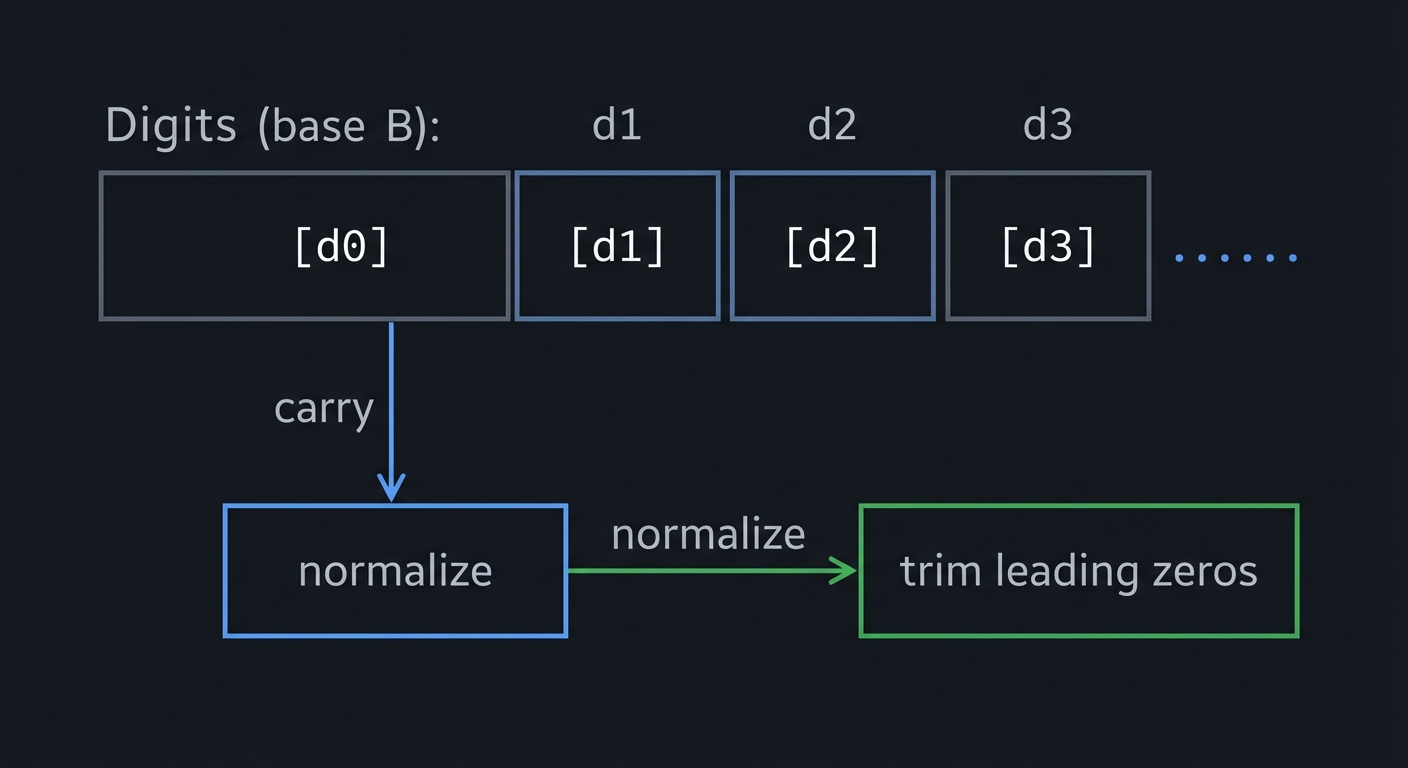
The Core Question You’re Answering

“How do you perform exact arithmetic beyond machine word size while staying fast enough for real workloads?”

Concepts You Must Understand First

Base representation and carry propagation
Normalization and sign handling
Long multiplication vs Karatsuba thresholds
Division and modular exponentiation

Questions to Guide Your Design

What base and digit size will you use (2^32, 2^64, 10^9)?
When do you switch from classical multiply to Karatsuba?
How will you represent negative values and zero?
Which operations require normalization after every step?

Thinking Exercise

Multiply 1234 x 5678 using base 100. Write the digits of each number, perform the grade-school multiply, and carry-normalize the result.

The Interview Questions They’ll Ask

Why is Karatsuba faster than classical multiplication?
How do you implement modular exponentiation efficiently?
What is the complexity of long division?
How do you avoid timing leaks in modular arithmetic?

Hints in Layers

Hint 1: Get Add/Sub Correct First If carry/borrow is wrong, everything else will fail.

Hint 2: Implement Multiply Next Classical O(n^2) multiplication is easiest to validate.

Hint 3: Add Division Using Algorithm D Start with positive integers only, then add sign support.

Hint 4: Add ModExp and GCD These let you build RSA and primality tests.

Books That Will Help

Topic	Book	Chapter
Multiple precision	TAOCP Vol 2	Ch. 4
Integer representation	CS:APP	Ch. 2
Divide and conquer	Algorithms, 4th Edition	Ch. 2.3
Low-level arithmetic	Write Great Code, Vol. 2	Ch. 7

Common Pitfalls & Debugging

Problem: “Results contain random extra digits”

Why: Leading zeros not trimmed or size not updated.
Fix: Normalize after every operation and strip leading zeros.
Quick test: Add a number to itself and compare sizes.

Problem: “Negative subtraction gives wrong sign”

Why: Comparing magnitudes incorrectly before subtracting.
Fix: Compare absolute values and swap operands when needed.
Quick test: Verify (a - b) + b = a for random a,b.

Implementation Hints:

BigNum representation:

typedef struct {
    uint32_t* digits;  // Array of "digits" (base 2^32)
    size_t size;       // Number of digits
    int sign;          // +1 or -1
} BigNum;

// Example: 12345678901234567890
// In base 2^32 ≈ 4.29 billion
// = 2 * (2^32)^1 + 3755744766 * (2^32)^0

Classical addition:

void bignum_add(BigNum* result, BigNum* a, BigNum* b) {
    uint64_t carry = 0;
    for (size_t i = 0; i < max(a->size, b->size); i++) {
        uint64_t sum = carry;
        if (i < a->size) sum += a->digits[i];
        if (i < b->size) sum += b->digits[i];
        result->digits[i] = (uint32_t)sum;
        carry = sum >> 32;
    }
    if (carry) result->digits[result->size++] = carry;
}

Karatsuba multiplication:

To multiply x and y (n digits each):
1. Split: x = x1 * B + x0, y = y1 * B + y0  (B = base^(n/2))
2. Compute:
   z0 = x0 * y0
   z2 = x1 * y1
   z1 = (x0 + x1) * (y0 + y1) - z0 - z2
3. Result: z2 * B² + z1 * B + z0

Complexity: O(n^1.585) instead of O(n²)

Algorithm D (division):

Knuth's Algorithm D is the classical long division algorithm:
1. Normalize divisor (shift so leading digit >= base/2)
2. For each digit of quotient:
   a. Estimate quotient digit
   b. Multiply back and subtract
   c. Correct if estimate was wrong

Learning milestones:

Addition/subtraction work → You understand carry propagation
Karatsuba is faster for large numbers → You understand divide-and-conquer
Division works correctly → You’ve mastered Algorithm D
RSA encryption works → You can do cryptography!

Definition of Done

All arithmetic operations correct against a reference
Karatsuba beats classical beyond a measured threshold
Modexp and GCD work on large inputs
Toy RSA encrypt/decrypt round-trip succeeds

Project 7: Floating-Point Emulator

File: LEARN_TAOCP_DEEP_DIVE.md
Main Programming Language: C
Alternative Programming Languages: Rust, C++
Coolness Level: Level 4: Hardcore Tech Flex
Business Potential: 2. The “Micro-SaaS / Pro Tool”
Difficulty: Level 4: Expert
Knowledge Area: Floating-Point / IEEE 754 / Numerical Analysis
Software or Tool: Building: Soft Float Library
Main Book: “The Art of Computer Programming, Volume 2” Section 4.2 - Knuth

What you’ll build: A software floating-point library that implements IEEE 754 arithmetic from scratch—addition, subtraction, multiplication, division, and rounding modes.

Why it teaches TAOCP: Section 4.2 covers floating-point arithmetic in detail. Understanding how floats work at the bit level is crucial for numerical programming. You’ll finally understand why 0.1 + 0.2 ≠ 0.3.

Core challenges you’ll face:

Encoding/decoding IEEE 754 format → maps to representation
Alignment and normalization → maps to floating-point addition
Rounding modes → maps to precision control
Special values (NaN, Inf) → maps to exception handling

Key Concepts:

Floating-Point Representation: TAOCP Vol 2, Section 4.2.1
Floating-Point Addition: TAOCP Vol 2, Section 4.2.1
Floating-Point Multiplication: TAOCP Vol 2, Section 4.2.1
Accuracy: TAOCP Vol 2, Section 4.2.2

Difficulty: Expert Time estimate: 2 weeks Prerequisites:

Project 6 (arbitrary precision) helpful
Understanding of binary fractions
Knowledge of IEEE 754 format

Real world outcome:

$ ./softfloat

# Decode IEEE 754
float> decode 0x40490FDB
Sign: 0 (positive)
Exponent: 10000000 (bias 127, actual = 1)
Mantissa: 10010010000111111011011
Value: 3.14159265... (pi approximation)

# Why 0.1 + 0.2 != 0.3
float> exact 0.1
0.1 decimal = 0.00011001100110011001100110011001... binary (repeating!)
Stored as: 0.100000001490116119384765625

float> 0.1 + 0.2
= 0.30000000000000004 (not exactly 0.3!)

# Rounding modes
float> mode round_nearest
float> 1.0 / 3.0
= 0.3333333432674408 (rounded to nearest)

float> mode round_toward_zero
float> 1.0 / 3.0
= 0.3333333134651184 (truncated)

# Special values
float> 1.0 / 0.0
= +Infinity

float> 0.0 / 0.0
= NaN (Not a Number)

Visual Model

[S][Exponent][Mantissa]
 1   8 bits     23 bits
value = (-1)^S * 1.M * 2^(E-bias)

The Core Question You’re Answering

“How do floating-point numbers represent real values, and where do the errors come from?”

Concepts You Must Understand First

Exponent bias and hidden leading 1
Alignment, normalization, and rounding
Denormals, infinities, and NaNs
Guard, round, and sticky bits

Questions to Guide Your Design

How will you handle rounding modes consistently?
What precision do you keep during intermediate steps?
How will you encode and decode NaN payloads?
What happens on overflow or underflow?

Thinking Exercise

Convert 0.1 to binary and find the nearest representable 32-bit float. Compare it to decimal 0.1 and compute the error.

The Interview Questions They’ll Ask

Why does 0.1 + 0.2 not equal 0.3 in binary floats?
What is a denormal number and why does it exist?
How do rounding modes affect reproducibility?
What is NaN, and how is it propagated?

Hints in Layers

Hint 1: Start With Decode/Encode Being able to parse bits correctly is the foundation.

Hint 2: Implement Addition With Alignment Handle exponent shifts before mantissa add/sub.

Hint 3: Add Rounding Use guard/round/sticky bits to implement IEEE rules.

Hint 4: Add Special Cases Handle NaN, Inf, and denormals last.

Books That Will Help

Topic	Book	Chapter
Floating-point	TAOCP Vol 2	Ch. 4.2
Number representation	CS:APP	Ch. 2
Computer arithmetic	Computer Organization and Design	Ch. 3
Low-level arithmetic	Write Great Code, Vol. 2	Ch. 7

Common Pitfalls & Debugging

Problem: “Rounding off by 1 ULP”

Why: Missing sticky bit or wrong tie-breaking rule.
Fix: Track guard/round/sticky and implement round-to-even.
Quick test: Compare against hardware results for edge cases.

Problem: “NaNs collapse to zero”

Why: Treating NaN as a normal value during normalization.
Fix: Short-circuit when exponent is all 1s and mantissa != 0.
Quick test: NaN op NaN should yield NaN, not 0.

Implementation Hints:

IEEE 754 single precision (32-bit):

Bit layout: [S][EEEEEEEE][MMMMMMMMMMMMMMMMMMMMMMM]
            [1][ 8 bits ][       23 bits        ]

S = sign (0 = positive, 1 = negative)
E = biased exponent (actual = E - 127)
M = mantissa (implicit leading 1)

Value = (-1)^S × 1.M × 2^(E-127)

Special cases:
  E=0, M=0: Zero (±0)
  E=0, M≠0: Denormalized (0.M × 2^-126)
  E=255, M=0: Infinity (±∞)
  E=255, M≠0: NaN

Floating-point addition:

add(a, b):
Align exponents: shift smaller mantissa right
Add mantissas (with implicit 1)
Normalize: if overflow, shift right, increment exponent
                  if leading zeros, shift left, decrement exponent
Round mantissa to 23 bits
Handle overflow/underflow

Rounding modes:

Round to nearest (even): Default, unbiased
Round toward zero: Truncate
Round toward +∞: Always round up
Round toward -∞: Always round down

Learning milestones:

Encode/decode works → You understand representation
Addition handles alignment → You understand the algorithm
0.1 + 0.2 behaves correctly → You understand precision limits
All rounding modes work → You understand IEEE 754 fully

Definition of Done

Encode/decode matches IEEE 754 for known values
Arithmetic matches hardware for a test corpus
All rounding modes produce expected results
NaN/Inf/denormal cases behave correctly

VOLUME 3: SORTING AND SEARCHING

Project 8: Complete Sorting Algorithm Collection

File: LEARN_TAOCP_DEEP_DIVE.md
Main Programming Language: C
Alternative Programming Languages: Rust, Go
Coolness Level: Level 3: Genuinely Clever
Business Potential: 2. The “Micro-SaaS / Pro Tool”
Difficulty: Level 3: Advanced
Knowledge Area: Sorting / Algorithm Analysis
Software or Tool: Building: Sort Library
Main Book: “The Art of Computer Programming, Volume 3” Chapter 5 - Knuth

What you’ll build: Every major sorting algorithm from TAOCP Chapter 5—insertion sort, shellsort, heapsort, quicksort, merge sort, radix sort—with instrumentation to count comparisons and moves.

Why it teaches TAOCP: Chapter 5 is the definitive reference on sorting. Knuth analyzes each algorithm mathematically, proving their complexity. You’ll understand not just how, but why each algorithm behaves as it does.

Core challenges you’ll face:

Implementing all major algorithms → maps to algorithm diversity
Counting comparisons accurately → maps to algorithm analysis
Choosing optimal shellsort gaps → maps to gap sequences
Quicksort pivot selection → maps to randomization

Key Concepts:

Insertion Sort: TAOCP Vol 3, Section 5.2.1
Shellsort: TAOCP Vol 3, Section 5.2.1
Heapsort: TAOCP Vol 3, Section 5.2.3
Quicksort: TAOCP Vol 3, Section 5.2.2
Merge Sort: TAOCP Vol 3, Section 5.2.4
Radix Sort: TAOCP Vol 3, Section 5.2.5
Minimum Comparisons: TAOCP Vol 3, Section 5.3

Difficulty: Advanced Time estimate: 2-3 weeks Prerequisites:

Basic algorithm knowledge
C programming
Understanding of recursion

Real world outcome:

$ ./sort_suite benchmark --size 100000

Algorithm       | Time    | Comparisons  | Moves     | Stable?
----------------|---------|--------------|-----------|--------
Insertion Sort  | 2.34s   | 2,500,125,000| 2,500,124,999| Yes
Shell Sort      | 0.023s  | 2,341,567    | 2,341,567 | No
Heap Sort       | 0.021s  | 2,567,891    | 1,123,456 | No
Quick Sort      | 0.015s  | 1,789,234    | 567,123   | No
Merge Sort      | 0.019s  | 1,660,964    | 1,660,964 | Yes
Radix Sort      | 0.008s  | 0            | 800,000   | Yes

Theoretical minimums for n=100,000:
  Comparisons: n log₂ n - 1.44n ≈ 1,560,000
  Merge sort achieves: 1,660,964 (within 6%!)

$ ./sort_suite visualize quicksort
[Animated ASCII visualization of quicksort partitioning...]

Visual Model

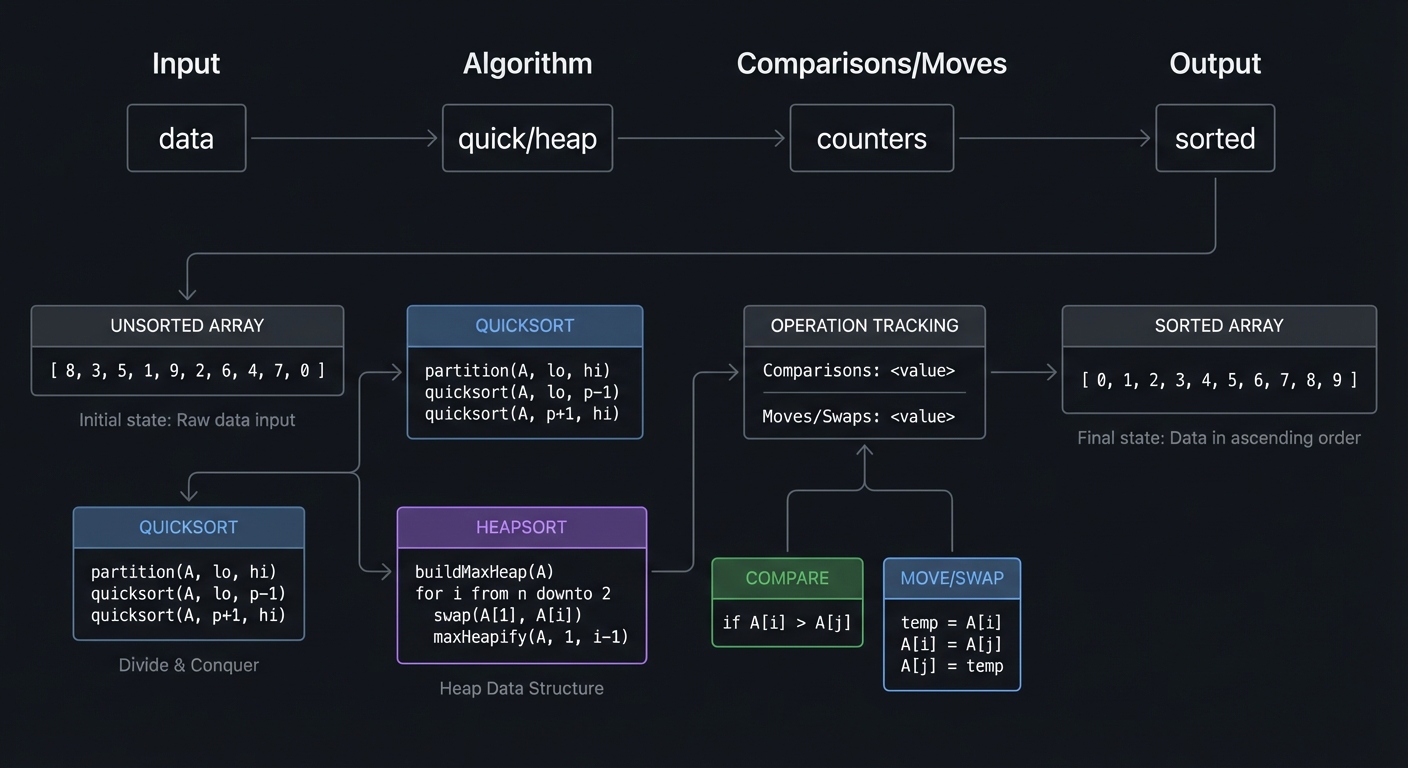
Input -> Algorithm -> Comparisons/Moves -> Output
  |         |              |               |
 data    quick/heap      counters        sorted

taocp sorting pipeline

The Core Question You’re Answering

“Why do different sorting algorithms behave so differently on the same data, and how do you predict it?”

Concepts You Must Understand First

Stability and in-place constraints
Average vs worst-case behavior
Comparison vs distribution sorting
Input distribution effects (nearly sorted, reversed, random)

Questions to Guide Your Design

How will you count comparisons and moves consistently across algorithms?
What data sets will you use to expose best/worst cases?
Which algorithms share helper routines (partition, heapify)?
How will you visualize and compare results fairly?

Thinking Exercise

Count the comparisons made by insertion sort on [3,1,2]. Then run your instrumentation to verify.

The Interview Questions They’ll Ask

Why is quicksort fast on average but risky in worst case?
What makes a sort stable, and why does it matter?
When is radix sort better than comparison sorts?
How do you choose a sort for nearly-sorted data?

Hints in Layers

Hint 1: Implement Insertion, Merge, Heap First These give you stable and worst-case guarantees.

Hint 2: Add Quicksort with Good Pivoting Use median-of-three or randomized pivots.

Hint 3: Add Shell and Radix Compare comparison-based to distribution-based sorts.

Hint 4: Instrument Every Operation Wrap comparisons and moves in macros.

Books That Will Help

Topic	Book	Chapter
Sorting analysis	TAOCP Vol 3	Ch. 5
Practical sorting	Algorithms in C	Part 3
Complexity insights	Algorithms, 4th Edition	Ch. 2
Data movement	Computer Systems: A Programmer’s Perspective	Ch. 6

Common Pitfalls & Debugging

Problem: “Comparison counts don’t match theory”

Why: Counting extra comparisons in loop conditions.
Fix: Wrap only the value comparisons, not loop checks.
Quick test: Validate on tiny arrays with known counts.

Problem: “Quicksort blows stack”

Why: Worst-case recursion depth from bad pivots.
Fix: Use tail recursion elimination or always recurse on smaller partition.
Quick test: Sort already sorted input and ensure depth stays small.

Implementation Hints:

Shellsort with good gap sequence:

// Knuth's sequence: 1, 4, 13, 40, 121, ... (3^k - 1)/2
void shellsort(int* a, int n) {
    int gap = 1;
    while (gap < n/3) gap = gap * 3 + 1;

    while (gap >= 1) {
        for (int i = gap; i < n; i++) {
            for (int j = i; j >= gap && a[j] < a[j-gap]; j -= gap) {
                swap(&a[j], &a[j-gap]);
            }
        }
        gap /= 3;
    }
}

Quicksort with median-of-three:

int partition(int* a, int lo, int hi) {
    // Median of three pivot selection
    int mid = lo + (hi - lo) / 2;
    if (a[mid] < a[lo]) swap(&a[mid], &a[lo]);
    if (a[hi] < a[lo]) swap(&a[hi], &a[lo]);
    if (a[mid] < a[hi]) swap(&a[mid], &a[hi]);
    int pivot = a[hi];

    int i = lo;
    for (int j = lo; j < hi; j++) {
        if (a[j] < pivot) {
            swap(&a[i], &a[j]);
            i++;
        }
    }
    swap(&a[i], &a[hi]);
    return i;
}

Heapsort:

1. Build max-heap in O(n) using bottom-up heapify
2. Repeatedly:
   a. Swap root (maximum) with last element
   b. Reduce heap size by 1
   c. Heapify root down

Advantage: O(n log n) worst case, in-place
Disadvantage: Not stable, more comparisons than quicksort

Learning milestones:

All algorithms implemented correctly → You understand sorting
Comparison counts match theory → You understand analysis
Can predict which is best for given data → You understand trade-offs
Can explain each algorithm’s invariant → You truly understand sorting

Definition of Done

All algorithms sort correctly across input distributions
Comparison/move counters match small known cases
Benchmarks show expected average/worst-case trends
Stability verified for stable algorithms

Project 9: Search Tree Collection (BST, AVL, B-Trees)

File: LEARN_TAOCP_DEEP_DIVE.md
Main Programming Language: C
Alternative Programming Languages: Rust, C++
Coolness Level: Level 4: Hardcore Tech Flex
Business Potential: 3. The “Service & Support” Model
Difficulty: Level 4: Expert
Knowledge Area: Search Trees / Balancing / Databases
Software or Tool: Building: Tree Library
Main Book: “The Art of Computer Programming, Volume 3” Section 6.2 - Knuth

What you’ll build: A complete collection of search trees—binary search trees, AVL trees, red-black trees (as 2-3-4 tree representation), and B-trees for disk-based storage.

Why it teaches TAOCP: Section 6.2 covers tree-based searching exhaustively. You’ll understand not just how to implement balanced trees, but the mathematics behind their height guarantees and why B-trees are optimal for disks.

Core challenges you’ll face:

AVL rotations → maps to balance maintenance
B-tree split and merge → maps to multi-way trees
Red-black coloring rules → maps to 2-3-4 tree correspondence
Disk-optimized operations → maps to I/O efficiency

Key Concepts:

Binary Search Trees: TAOCP Vol 3, Section 6.2.2
AVL Trees: TAOCP Vol 3, Section 6.2.3
B-Trees: TAOCP Vol 3, Section 6.2.4
Optimal BSTs: TAOCP Vol 3, Section 6.2.2

Difficulty: Expert Time estimate: 3-4 weeks Prerequisites:

Project 4 (basic trees)
Understanding of tree rotations
Binary search knowledge

Real world outcome:

$ ./tree_collection

# Compare tree heights
tree> insert_random 10000
AVL tree:
  Nodes: 10000
  Height: 14
  Theoretical max: 1.44 log₂(10001) ≈ 19.2
  Actual/max: 73% (well balanced!)

B-tree (order 100):
  Nodes: 10000
  Height: 2
  Minimum height: log₁₀₀(10000) = 2 ✓

# Visualize rotations
tree> insert_avl_trace 5 3 7 2 4 6 8 1
Inserting 5: Root is 5
Inserting 3: Left of 5
Inserting 7: Right of 5
Inserting 2: Left of 3
Inserting 4: Right of 3
Inserting 6: Left of 7
Inserting 8: Right of 7
Inserting 1: Left of 2
  Balance factor of 3 is now 2 (left-heavy)
  Performing RIGHT rotation at 3:
       5              5
      / \            / \
     3   7    →     2   7
    / \            / \
   2   4          1   3
  /                    \
 1                      4

# B-tree disk operations
tree> btree_create "index.db" order=100
tree> btree_insert_bulk data.csv
Inserted 1,000,000 keys
Disk reads: 3 per lookup (height 3)

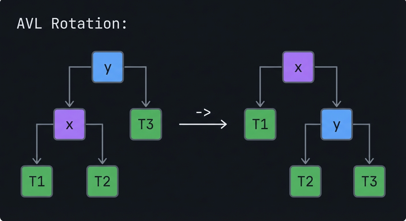
Visual Model

AVL Rotation:
   y            x
  / \          / \
 x   T3  ->   T1  y
/ \              / \
T1 T2            T2 T3

taocp avl rotation

The Core Question You’re Answering

“How do balanced trees guarantee log-time operations, and why do B-trees dominate disk-based storage?”

Concepts You Must Understand First

Tree height invariants and balance factors
Rotations (single and double)
B-tree node capacity and split/merge
Disk I/O model (block size vs height)

Questions to Guide Your Design

How will you store parent pointers and node metadata?
When do you trigger rotations or splits?
How will you persist B-tree nodes to disk?
What tests confirm height bounds for each tree?

Thinking Exercise

Insert 10, 20, 30 into an AVL tree. Show the rotation and the final shape.

The Interview Questions They’ll Ask

Compare AVL trees to red-black trees.
Why are B-trees ideal for disks or SSDs?
How do you implement a B-tree split?
What is the amortized cost of rebalancing?

Hints in Layers

Hint 1: Build a Correct BST First If your BST is wrong, rotations will not fix it.

Hint 2: Add AVL Rotations Implement single rotations, then double rotations.

Hint 3: Implement B-Tree Insert Handle splitting a full node before descent.

Hint 4: Add Disk Simulation Count block reads/writes to validate I/O efficiency.

Books That Will Help

Topic	Book	Chapter
Balanced trees	TAOCP Vol 3	Ch. 6.2
Search trees	Algorithms, 4th Edition	Ch. 3
Disk-based structures	Algorithms in C	Part 5
Data layout	Computer Organization and Design	Ch. 5

Common Pitfalls & Debugging

Problem: “AVL height metadata is wrong”

Why: Not updating heights after rotations.
Fix: Recompute heights bottom-up for affected nodes only.
Quick test: Validate balance factors for every node after inserts.

Problem: “B-tree insert corrupts structure”

Why: Split logic does not move the median key correctly.
Fix: Carefully copy left/right halves and promote the median.
Quick test: After each insert, traverse nodes and verify key ordering.

Implementation Hints:

AVL rotation:

Node* rotate_right(Node* y) {
    Node* x = y->left;
    Node* T = x->right;

    x->right = y;
    y->left = T;

    y->height = 1 + max(height(y->left), height(y->right));
    x->height = 1 + max(height(x->left), height(x->right));

    return x;  // New root
}

int balance_factor(Node* n) {
    return height(n->left) - height(n->right);
}

// After insert, walk back up and rebalance
// |balance_factor| > 1 means rotation needed

B-tree structure:

#define ORDER 100  // Max children per node

typedef struct BTreeNode {
    int num_keys;
    int keys[ORDER - 1];
    void* values[ORDER - 1];
    struct BTreeNode* children[ORDER];
    bool is_leaf;
} BTreeNode;

// Invariants:
// - All leaves at same depth
// - Each node has ceil(ORDER/2) to ORDER children
// - Each node has ceil(ORDER/2)-1 to ORDER-1 keys

B-tree split:

When inserting into full node:
Split node into two nodes
Median key moves up to parent
Left half goes to left child
Right half goes to right child
May recursively split parent

Learning milestones:

BST operations work → You understand tree searching
AVL maintains balance → You understand rotations
B-tree has optimal height → You understand disk optimization
Can implement red-black via 2-3-4 → You understand the connection

Definition of Done

BST/AVL/B-tree insert/find/delete pass tests
AVL height bounds hold across random inputs
B-tree split/merge logic preserves invariants
Disk I/O model shows expected lookup costs

Project 10: Hash Table Laboratory

File: LEARN_TAOCP_DEEP_DIVE.md
Main Programming Language: C
Alternative Programming Languages: Rust, Go
Coolness Level: Level 3: Genuinely Clever
Business Potential: 3. The “Service & Support” Model
Difficulty: Level 3: Advanced
Knowledge Area: Hashing / Collision Resolution / Analysis
Software or Tool: Building: Hash Table Library
Main Book: “The Art of Computer Programming, Volume 3” Section 6.4 - Knuth

What you’ll build: A comprehensive hash table library implementing multiple collision resolution strategies—chaining, linear probing, quadratic probing, double hashing—with analysis tools.

Why it teaches TAOCP: Section 6.4 is the definitive analysis of hashing. Knuth derives the expected number of probes for each method, explains why load factor matters, and proves when linear probing clusters. You’ll understand hashing at the mathematical level.

Core challenges you’ll face:

Choosing good hash functions → maps to distribution quality
Primary clustering in linear probing → maps to collision analysis
Deletion in open addressing → maps to tombstones
Universal hashing → maps to randomized algorithms

Key Concepts:

Hash Functions: TAOCP Vol 3, Section 6.4
Chaining: TAOCP Vol 3, Section 6.4
Open Addressing: TAOCP Vol 3, Section 6.4
Analysis of Hashing: TAOCP Vol 3, Section 6.4

Difficulty: Advanced Time estimate: 2 weeks Prerequisites:

Basic hash table understanding
Modular arithmetic
Probability basics

Real world outcome:

$ ./hash_lab

# Compare collision strategies
hash> benchmark chaining linear quadratic double --size 100000 --load 0.75

Method          | Avg Probes (success) | Avg Probes (failure)
----------------|----------------------|---------------------
Chaining        | 1.375               | 0.750
Linear Probing  | 2.500               | 8.500
Quadratic Probe | 1.833               | 3.188
Double Hashing  | 1.625               | 2.627

Theoretical (Knuth's formulas at α=0.75):
  Linear (success): 1/2 * (1 + 1/(1-α)²) = 2.5 ✓
  Linear (failure): 1/2 * (1 + 1/(1-α)²) = 8.5 ✓
  Double (success): -ln(1-α)/α = 1.85 ✓
  Double (failure): 1/(1-α) = 4.0

# Visualize clustering
hash> visualize linear --load 0.7
[##..###.#.##...####.#.##..###...####..#]
  ↑       ↑
  Clusters form!

hash> visualize double --load 0.7
[.#.#.#..#.#.#.##.#..#.#..#.##.#.#.#..#]
  ↑
  Much more uniform!

# Test hash function quality
hash> test_hash "fnv1a" 1000000
Chi-square uniformity test: PASS (p=0.73)
Avalanche test: 49.8% bit changes (ideal: 50%)

Visual Model

key -> hash -> index -> probe sequence
             |        |-> slot -> found
             |        |-> slot -> next probe

taocp hash probe flow

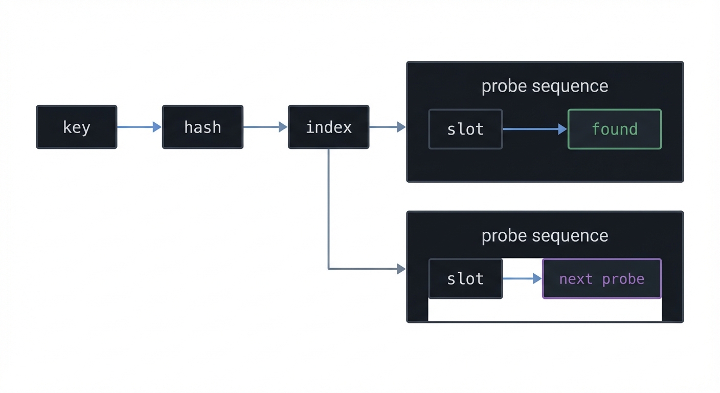
The Core Question You’re Answering

“How do hash tables provide near-constant time, and what breaks that promise?”

Concepts You Must Understand First

Hash function distribution and avalanche
Load factor and expected probes
Clustering in open addressing
Tombstones and rehashing

Questions to Guide Your Design

How will you select or design hash functions for different key types?
When do you resize and rehash the table?
How do you handle deletions without breaking probe sequences?
How will you measure probe counts accurately?

Thinking Exercise

Use a table of size 11 and linear probing. Insert keys with hashes 1, 12, 23, 34 and write the final table.

The Interview Questions They’ll Ask

Why does linear probing create clusters?
What is the expected probe count for double hashing?
How do you delete in open addressing safely?
What makes a hash function good?

Hints in Layers

Hint 1: Implement Chaining First It is the easiest to get correct and test.

Hint 2: Add Linear Probing Start with insert/search only, then add deletion.

Hint 3: Add Double Hashing Use a second hash that is never zero.

Hint 4: Instrument Everything Track probes and compare to Knuth’s formulas.

Books That Will Help

Topic	Book	Chapter
Hashing analysis	TAOCP Vol 3	Ch. 6.4
Practical hash tables	Algorithms in C	Part 3
Randomization	Concrete Mathematics	Ch. 1
Systems perspective	Computer Systems: A Programmer’s Perspective	Ch. 2

Common Pitfalls & Debugging

Problem: “Search misses keys that exist”

Why: Deletion cleared slots instead of marking tombstones.
Fix: Use tombstones and rehash when too many accumulate.
Quick test: Insert, delete, reinsert, then search the old cluster.

Problem: “Table fills and loops forever”

Why: Probe sequence does not cover all slots.
Fix: Ensure step size is coprime to table size.
Quick test: Insert size-1 keys and verify you can still find each.

Implementation Hints:

Linear probing:

int linear_probe(HashTable* ht, Key key) {
    int h = hash(key) % ht->size;
    while (ht->table[h].occupied) {
        if (ht->table[h].key == key) return h;  // Found
        h = (h + 1) % ht->size;  // Linear step
    }
    return -h - 1;  // Not found, insert position
}

// Primary clustering: long runs form
// Expected probes: 1/2 (1 + 1/(1-α)²) where α = load factor

Double hashing:

int double_hash(HashTable* ht, Key key) {
    int h1 = hash1(key) % ht->size;
    int h2 = 1 + (hash2(key) % (ht->size - 1));  // Never 0!

    int h = h1;
    while (ht->table[h].occupied) {
        if (ht->table[h].key == key) return h;
        h = (h + h2) % ht->size;  // Different step per key
    }
    return -h - 1;
}

// No clustering! Different keys take different paths
// Expected probes: -ln(1-α)/α

Deletion with tombstones:

void delete(HashTable* ht, Key key) {
    int pos = find(ht, key);
    if (pos >= 0) {
        ht->table[pos].deleted = true;  // Tombstone, not empty
    }
}

// Tombstones allow continued probing
// But too many tombstones hurt performance
// Need periodic rehashing to clean them up

Learning milestones:

All collision strategies work → You understand hashing basics
Probe counts match theory → You understand analysis
Clustering is visible → You understand why double hashing is better
Deletion works correctly → You understand tombstones

Definition of Done

Chaining and open addressing operations pass tests
Probe counts align with Knuth’s formulas
Deletion with tombstones preserves find correctness
Hash quality tests show near-uniform distribution

VOLUME 4: COMBINATORIAL ALGORITHMS

Project 11: Combinatorial Object Generator

File: LEARN_TAOCP_DEEP_DIVE.md
Main Programming Language: C
Alternative Programming Languages: Rust, Python
Coolness Level: Level 4: Hardcore Tech Flex
Business Potential: 2. The “Micro-SaaS / Pro Tool”
Difficulty: Level 3: Advanced
Knowledge Area: Combinatorics / Enumeration / Generation
Software or Tool: Building: Combinatorics Library
Main Book: “The Art of Computer Programming, Volume 4A” Section 7.2.1 - Knuth

What you’ll build: A library that generates all combinatorial objects—tuples, permutations, combinations, partitions, set partitions—using the elegant algorithms from TAOCP.

Why it teaches TAOCP: Section 7.2.1 covers how to systematically generate every possible object of a given type. These algorithms are the foundation for exhaustive search, testing, and combinatorial optimization.

Core challenges you’ll face:

Gray code for tuples → maps to minimal change generation
Heap’s algorithm for permutations → maps to efficient swapping
Revolving door for combinations → maps to adjacent transposition
Integer partitions → maps to number theory

Key Concepts:

Generating Tuples: TAOCP Vol 4A, Section 7.2.1.1
Generating Permutations: TAOCP Vol 4A, Section 7.2.1.2
Generating Combinations: TAOCP Vol 4A, Section 7.2.1.3
Generating Partitions: TAOCP Vol 4A, Section 7.2.1.4

Difficulty: Advanced Time estimate: 2 weeks Prerequisites:

Understanding of recursion
Basic combinatorics
C programming

Real world outcome:

$ ./combinatorics

# Generate binary strings (Gray code)
combo> tuples binary 4 --gray
0000 → 0001 → 0011 → 0010 → 0110 → 0111 → 0101 → 0100 →
1100 → 1101 → 1111 → 1110 → 1010 → 1011 → 1001 → 1000
Note: Each differs from previous by exactly 1 bit!

# Generate permutations (Heap's algorithm)
combo> permutations 4 --heap
1234 → 2134 → 3124 → 1324 → 2314 → 3214 →
3241 → 2341 → 1342 → 3142 → 2143 → 1243 →
1423 → 4123 → 2413 → 1432 → 4132 → 3412 →
4312 → 3421 → 4321 → 2431 → 4231 → 3241
Note: Each differs from previous by single swap!

# Generate combinations (revolving door)
combo> combinations 5 3 --revolving
{1,2,3} → {1,2,4} → {1,3,4} → {2,3,4} → {2,3,5} →
{1,3,5} → {1,2,5} → {1,4,5} → {2,4,5} → {3,4,5}
Note: Each differs by adding one element and removing one!

# Integer partitions
combo> partitions 10
10 = 10
   = 9+1 = 8+2 = 8+1+1 = 7+3 = 7+2+1 = ...
   = 1+1+1+1+1+1+1+1+1+1
Total: 42 partitions (p(10) = 42)

Visual Model

Generate -> Next Object -> Minimal Change -> Repeat
   |             |             |             |
  rules       output         delta        count

taocp generation pipeline

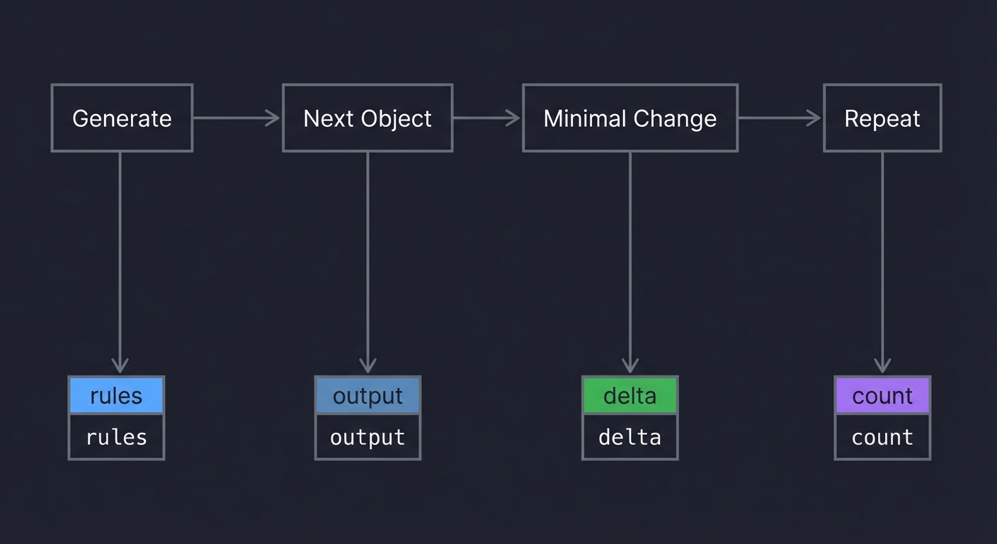
The Core Question You’re Answering

“How can you enumerate combinatorial objects without duplicates and with minimal changes between steps?”

Concepts You Must Understand First

Gray code and minimal change sequences
Permutation generation algorithms
Combination ordering and revolving door method
Integer partitions and recurrence counts

Questions to Guide Your Design

Will you generate objects iteratively or recursively?
How do you avoid duplicates and ensure full coverage?
How will you validate ordering properties (Gray code, adjacent swap)?
What is the memory footprint for large n?

Thinking Exercise

Generate all combinations of 4 choose 2 by hand and check that your algorithm produces the same sequence.

The Interview Questions They’ll Ask

How many permutations exist for n items?
What is the advantage of Gray code generation?
How do you generate combinations without recursion?
How do you compute the number of integer partitions?

Hints in Layers

Hint 1: Start With Recursive Generation It is easy to understand and validate.

Hint 2: Implement Gray Code by XOR Use i ^ (i » 1) to generate Gray codes.

Hint 3: Add Heap’s Algorithm Validate that each permutation differs by one swap.

Hint 4: Add Partition Generator Use a state machine to avoid recursion and reduce memory.

Books That Will Help

Topic	Book	Chapter
Combinatorial generation	TAOCP Vol 4A	Ch. 7.2.1
Recursion patterns	The Recursive Book of Recursion	Ch. 5-7
Algorithm design	Algorithms, 4th Edition	Ch. 1
Discrete math	Concrete Mathematics	Ch. 2

Common Pitfalls & Debugging

Problem: “Duplicate permutations appear”

Why: Swap logic or recursion base case is wrong.
Fix: Use a visited counter and assert total outputs = n!.
Quick test: For n=4, ensure exactly 24 permutations.

Problem: “Gray code flips more than one bit”

Why: Incorrect update rule.
Fix: Use gray(i) = i ^ (i » 1).
Quick test: Check Hamming distance between successive codes is 1.

Implementation Hints:

Gray code generation:

// To generate next Gray code from current n-bit binary b:
// Flip the rightmost bit that produces a new code
void next_gray(int* b, int n) {
    // Find position to flip
    int j = 0;
    while (j < n && b[j] == (need to flip)) j++;
    b[j] = 1 - b[j];  // Flip bit j
}

// Alternative: Gray code of integer i is i XOR (i >> 1)

Heap’s algorithm for permutations:

void heap_permute(int* a, int n) {
    int c[n];  // State stack
    memset(c, 0, sizeof(c));
    output(a);  // First permutation

    int i = 0;
    while (i < n) {
        if (c[i] < i) {
            if (i % 2 == 0) swap(&a[0], &a[i]);
            else swap(&a[c[i]], &a[i]);
            output(a);  // Next permutation
            c[i]++;
            i = 0;
        } else {
            c[i] = 0;
            i++;
        }
    }
}

Revolving door combinations:

Generate all k-subsets of {1,...,n} with minimal changes:
Each step: remove one element, add an adjacent one

C(n,k) combinations, each differs by one "swap"
Used in: Ordering combinations for systematic testing

Learning milestones:

Gray code differs by 1 bit → You understand minimal change
Heap’s uses only swaps → You understand efficient generation
Can generate any combinatorial object → You understand the patterns
Counts match theoretical formulas → You verify correctness

Definition of Done

Counts match formulas for permutations/combinations
Gray code differs by exactly one bit each step
Revolving-door combinations differ by one swap
Partition counts match known values

Project 12: Dancing Links SAT Solver

File: LEARN_TAOCP_DEEP_DIVE.md
Main Programming Language: C
Alternative Programming Languages: Rust, C++
Coolness Level: Level 5: Pure Magic
Business Potential: 4. The “Open Core” Infrastructure
Difficulty: Level 5: Master
Knowledge Area: Backtracking / Exact Cover / SAT
Software or Tool: Building: Exact Cover Solver + SAT Solver
Main Book: “The Art of Computer Programming, Volume 4B” Section 7.2.2 - Knuth

What you’ll build: Knuth’s Dancing Links (DLX) algorithm for exact cover problems, plus a DPLL/CDCL SAT solver—the two most powerful general problem-solving techniques in Volume 4B.

Why it teaches TAOCP: Knuth calls these “two practical general problem solvers.” Dancing Links solves exact cover (Sudoku, N-Queens, polyomino puzzles). SAT solvers handle Boolean satisfiability (verification, planning, scheduling). Together, they can solve an enormous range of problems.

Core challenges you’ll face:

Implementing doubly-linked circular lists → maps to dancing links structure
Algorithm X with efficient covering/uncovering → maps to backtracking
Unit propagation in SAT → maps to constraint propagation
Conflict-driven clause learning → maps to CDCL

Key Concepts:

Dancing Links: TAOCP Vol 4B, Section 7.2.2.1
Exact Cover: Algorithm X from Knuth’s paper
DPLL Algorithm: TAOCP Vol 4B, Section 7.2.2.2
CDCL Enhancements: TAOCP Vol 4B, Section 7.2.2.2

Resources for key challenges:

Difficulty: Master Time estimate: 4-6 weeks Prerequisites:

Strong understanding of backtracking
Linked list expertise
Boolean logic

Real world outcome:

$ ./dlx_solver

# Solve Sudoku (as exact cover)
dlx> sudoku
5 3 . | . 7 . | . . .
6 . . | 1 9 5 | . . .
. 9 8 | . . . | . 6 .
------+-------+------
8 . . | . 6 . | . . 3
4 . . | 8 . 3 | . . 1
7 . . | . 2 . | . . 6
------+-------+------
. 6 . | . . . | 2 8 .
. . . | 4 1 9 | . . 5
. . . | . 8 . | . 7 9

Solving as exact cover problem...
Solution found in 0.001 seconds, 847 nodes explored:

5 3 4 | 6 7 8 | 9 1 2
6 7 2 | 1 9 5 | 3 4 8
1 9 8 | 3 4 2 | 5 6 7
------+-------+------
8 5 9 | 7 6 1 | 4 2 3
4 2 6 | 8 5 3 | 7 9 1
7 1 3 | 9 2 4 | 8 5 6
------+-------+------
9 6 1 | 5 3 7 | 2 8 4
2 8 7 | 4 1 9 | 6 3 5
3 4 5 | 2 8 6 | 1 7 9

# SAT solver
sat> load problem.cnf
Loaded 1000 variables, 4200 clauses

sat> solve
Running CDCL solver...
Propagations: 45,231
Conflicts: 892
Learned clauses: 634
Decision levels: max 47

SATISFIABLE
Solution: 1 -2 3 -4 5 ...

# Classic problems
dlx> n_queens 12
Found 14,200 solutions in 0.3 seconds

dlx> pentominos 6 10
Found 2,339 ways to tile 6x10 with 12 pentominoes

Visual Model

Exact Cover Matrix -> Cover -> Recurse -> Uncover -> Solution
        |              |          |         |          |
      columns       remove     search     restore    output

taocp exact cover flow

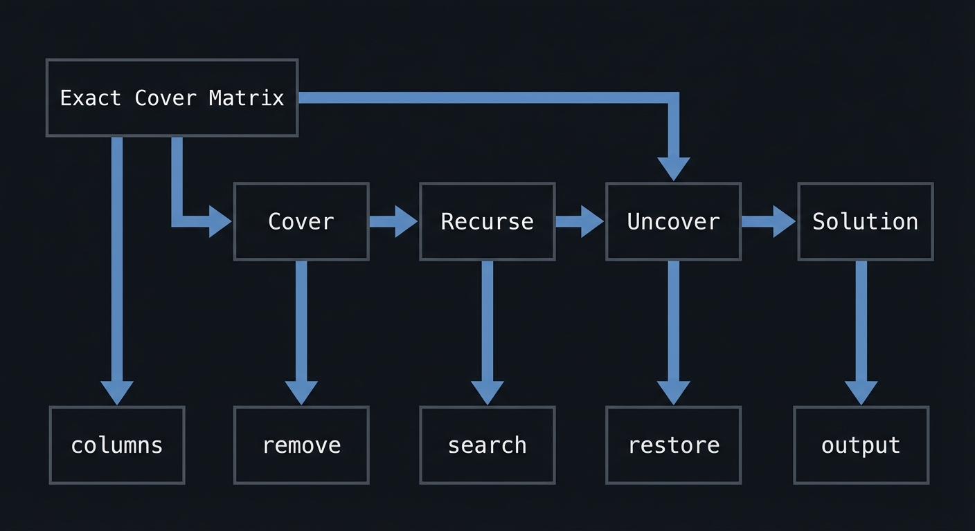
The Core Question You’re Answering

“How can backtracking be made fast enough to solve real problems like Sudoku and SAT?”

Concepts You Must Understand First

Exact cover formulation
Dancing Links cover/uncover operations
Unit propagation and decision levels
Clause learning and backjumping

Questions to Guide Your Design

How will you represent the sparse matrix efficiently?
Which heuristic picks the next column or variable?
How do you undo state changes without copying the world?
What metrics will you track (nodes explored, conflicts, learns)?

Thinking Exercise

Represent a 4x4 Sudoku as exact cover constraints. How many columns are required?

The Interview Questions They’ll Ask

Explain the cover and uncover operations in DLX.
What is the difference between DPLL and CDCL?
Why does the MRV heuristic speed up backtracking?
How do SAT solvers use clause learning?

Hints in Layers

Hint 1: Implement DLX First It is deterministic and easier to validate.

Hint 2: Add Sudoku as a Test It provides a reliable correctness target.

Hint 3: Implement DPLL Add unit propagation and pure literal elimination.

Hint 4: Add CDCL Start with conflict analysis and non-chronological backtracking.

Books That Will Help

Topic	Book	Chapter
Exact cover	TAOCP Vol 4B	Ch. 7.2.2
Backtracking	The Recursive Book of Recursion	Ch. 10
Data structures	Algorithms in C	Part 1
Logic foundations	Concrete Mathematics	Ch. 1

Common Pitfalls & Debugging

Problem: “Solver returns incorrect solutions”

Why: Cover/uncover order is not reversed properly.
Fix: Uncover in exact reverse order of cover.
Quick test: Run a known Sudoku and compare the unique solution.

Problem: “SAT solver loops or stalls”

Why: Unit propagation not applied after every assignment.
Fix: Re-run propagation after each decision or learn.
Quick test: Test a formula with unit clauses and verify immediate propagation.

Implementation Hints:

Dancing Links data structure:

typedef struct Node {
    struct Node* left;
    struct Node* right;
    struct Node* up;
    struct Node* down;
    struct Node* column;  // Column header
    int row_id;
} Node;

typedef struct Column {
    Node header;
    int size;    // Number of 1s in column
    char* name;  // Column identifier
} Column;

// Cover operation (temporarily remove column):
void cover(Column* c) {
    c->header.right->left = c->header.left;
    c->header.left->right = c->header.right;

    for (Node* i = c->header.down; i != &c->header; i = i->down) {
        for (Node* j = i->right; j != i; j = j->right) {
            j->down->up = j->up;
            j->up->down = j->down;
            j->column->size--;
        }
    }
}

// Uncover reverses everything (the "dance")
void uncover(Column* c) {
    // Reverse order of cover!
    for (Node* i = c->header.up; i != &c->header; i = i->up) {
        for (Node* j = i->left; j != i; j = j->left) {
            j->column->size++;
            j->down->up = j;
            j->up->down = j;
        }
    }
    c->header.right->left = &c->header;
    c->header.left->right = &c->header;
}

Algorithm X:

search(k):
    if no columns left: solution found!

    choose column c with minimum size (MRV heuristic)
    cover(c)

    for each row r in column c:
        include r in partial solution
        for each column j covered by r:
            cover(j)
        search(k+1)
        for each column j covered by r (reverse order):
            uncover(j)

    uncover(c)

DPLL with unit propagation:

DPLL(formula):
    unit_propagate()  // Set forced variables
    if conflict: return UNSAT

    if all clauses satisfied: return SAT

    pick unassigned variable x
    if DPLL(formula ∧ x): return SAT
    if DPLL(formula ∧ ¬x): return SAT
    return UNSAT

Learning milestones:

Can solve N-Queens with DLX → You understand exact cover
Sudoku solves in milliseconds → You understand efficient backtracking
SAT solver handles DIMACS files → You understand SAT solving
CDCL learns clauses effectively → You understand modern SAT techniques

Definition of Done

DLX solves Sudoku and N-Queens correctly
Exact-cover matrix builder validated with small puzzles
SAT solver reads DIMACS and returns correct SAT/UNSAT
CDCL stats (conflicts/learns) are reported

Project 13: Boolean Function Analyzer

File: LEARN_TAOCP_DEEP_DIVE.md
Main Programming Language: C
Alternative Programming Languages: Rust, Python
Coolness Level: Level 4: Hardcore Tech Flex
Business Potential: 3. The “Service & Support” Model
Difficulty: Level 4: Expert
Knowledge Area: Boolean Algebra / BDDs / Logic
Software or Tool: Building: BDD Library
Main Book: “The Art of Computer Programming, Volume 4A” Section 7.1 - Knuth

What you’ll build: A Boolean function analysis toolkit including truth table manipulation, Binary Decision Diagrams (BDDs), and satisfiability testing.

Why it teaches TAOCP: Section 7.1 covers “Zeros and Ones”—the foundation of digital logic. BDDs are a canonical form for Boolean functions, enabling efficient manipulation. This is essential for hardware verification, model checking, and symbolic computation.

Core challenges you’ll face:

Building BDDs with reduction → maps to canonical forms
BDD operations (AND, OR, NOT) → maps to function manipulation
Variable ordering heuristics → maps to complexity optimization
Counting satisfying assignments → maps to #SAT

Key Concepts:

Boolean Functions: TAOCP Vol 4A, Section 7.1.1
BDDs: TAOCP Vol 4A, Section 7.1.4
Bitwise Tricks: TAOCP Vol 4A, Section 7.1.3
Satisfiability: TAOCP Vol 4B, Section 7.2.2.2

Difficulty: Expert Time estimate: 2-3 weeks Prerequisites:

Boolean algebra
Graph/tree algorithms
Understanding of canonical forms

Real world outcome:

$ ./bdd_analyzer

# Build BDD for formula
bdd> build "(a & b) | (c & d)"
BDD created:
  Variables: 4
  Nodes: 5 (reduced from 15 in truth table)

bdd> visualize
    a
   / \
  b   c
 / \ / \
0   d   d
   / \ / \
  0   1   0   1

# Count satisfying assignments
bdd> count
6 satisfying assignments out of 16

# Apply operation
bdd> build "e & f"
bdd> or_bdds 1 2
New BDD: (a & b) | (c & d) | (e & f)
Nodes: 8

# Check equivalence
bdd> equiv "(a & b) | (a & c)" "a & (b | c)"
Functions are EQUIVALENT (BDDs identical after reduction)

# Find all solutions
bdd> all_sat
a=1,b=1,c=*,d=*,e=*,f=*  (covers 4 assignments)
a=0,b=*,c=1,d=1,e=*,f=*  (covers 4 assignments)
... (continues for all 6)

Visual Model

Formula -> BDD Reduce -> Canonical Graph
   |         |                 |
 variables  merge nodes      equivalence

taocp bdd pipeline

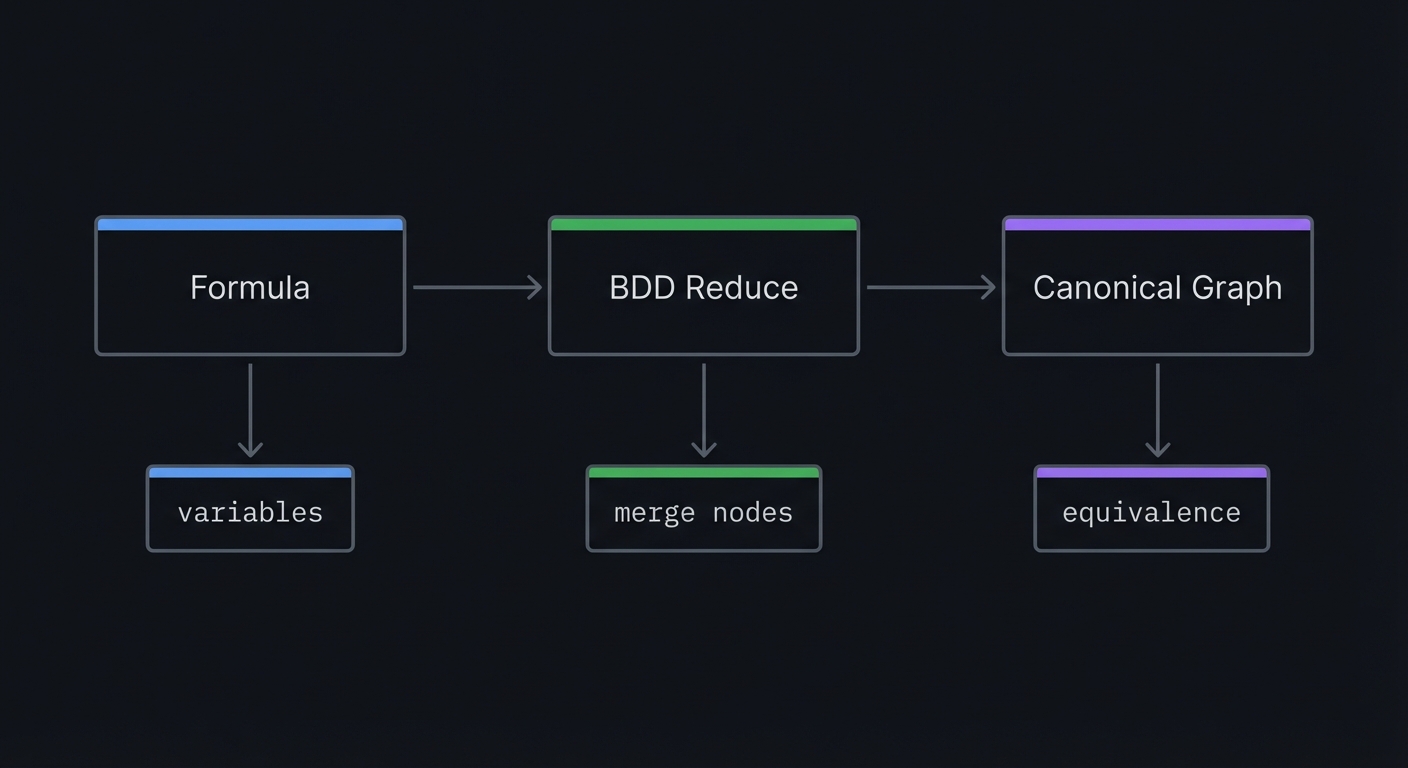
The Core Question You’re Answering

“How do canonical representations make Boolean reasoning fast and reliable?”

Concepts You Must Understand First

Boolean algebra and truth tables
BDD reduction rules (merge identical, remove redundant)
Unique table and memoization
Variable ordering impact on size

Questions to Guide Your Design

How will you enforce uniqueness of nodes?
What caching strategy prevents exponential recomputation?
How will you choose variable ordering for benchmarks?
How do you detect equivalence of two functions efficiently?

Thinking Exercise

Build BDDs for (a & b)

(a & c) and a & (b

c). Verify they reduce to the same graph.

The Interview Questions They’ll Ask

Why are BDDs canonical for a fixed variable order?
What happens to BDD size when variable order is poor?
How is ITE used to build all Boolean operations?
How would you count satisfying assignments with a BDD?

Hints in Layers

Hint 1: Build Terminal Nodes First ZERO and ONE should be singleton nodes.

Hint 2: Add Unique Table Ensure (var, low, high) returns a single node.

Hint 3: Implement ITE Everything else (AND/OR/NOT) can use it.

Hint 4: Add Memoization Cache ITE results to avoid exponential time.

Books That Will Help

Topic	Book	Chapter
Boolean functions	TAOCP Vol 4A	Ch. 7.1
Graph algorithms	Algorithms in C	Part 5
Logic foundations	Math for Programmers	Ch. 6
Discrete math	Concrete Mathematics	Ch. 1

Common Pitfalls & Debugging

Problem: “BDD size explodes”

Why: Variable order is poor or unique table is missing.
Fix: Try different orderings and confirm unique table use.
Quick test: Compare size for a simple function under two orders.

Problem: “Equivalence check fails”

Why: Two equivalent functions built with different variable orders.
Fix: Ensure identical ordering before comparing nodes.
Quick test: Build with same order and compare root pointers.

Implementation Hints:

BDD node structure:

typedef struct BDDNode {
    int var;              // Variable index
    struct BDDNode* low;  // False branch
    struct BDDNode* high; // True branch
} BDDNode;

// Terminal nodes
BDDNode* ZERO;  // Constant 0
BDDNode* ONE;   // Constant 1

// Unique table for canonicity
HashMap<(var, low, high) -> BDDNode*> unique_table;

ITE (If-Then-Else) operation:

BDDNode* ite(BDDNode* f, BDDNode* g, BDDNode* h) {
    // Terminal cases
    if (f == ONE) return g;
    if (f == ZERO) return h;
    if (g == ONE && h == ZERO) return f;
    if (g == h) return g;

    // Check computed cache
    if (cached(f, g, h)) return cache[f,g,h];

    // Find top variable
    int v = min_var(f, g, h);

    // Recursive calls
    BDDNode* low = ite(restrict(f, v, 0),
                       restrict(g, v, 0),
                       restrict(h, v, 0));
    BDDNode* high = ite(restrict(f, v, 1),
                        restrict(g, v, 1),
                        restrict(h, v, 1));

    // Build node (with unique table for reduction)
    BDDNode* result = make_node(v, low, high);
    cache[f,g,h] = result;
    return result;
}

BDD operations via ITE:

AND(f, g) = ITE(f, g, 0)
OR(f, g)  = ITE(f, 1, g)
NOT(f)    = ITE(f, 0, 1)
XOR(f, g) = ITE(f, NOT(g), g)

Learning milestones:

BDDs reduce correctly → You understand canonical forms
Operations work via ITE → You understand BDD algebra
Variable ordering affects size → You understand complexity
Can check equivalence instantly → You understand BDD power

Definition of Done

Unique table enforces canonical nodes
ITE-based operations match truth tables
Equivalence checks succeed on algebraic identities
BDD size varies predictably with variable ordering

Project 14: Bitwise Magic Toolkit

File: LEARN_TAOCP_DEEP_DIVE.md
Main Programming Language: C
Alternative Programming Languages: Rust, Assembly
Coolness Level: Level 4: Hardcore Tech Flex
Business Potential: 2. The “Micro-SaaS / Pro Tool”
Difficulty: Level 2: Intermediate
Knowledge Area: Bit Manipulation / Optimization
Software or Tool: Building: Bit Tricks Library
Main Book: “The Art of Computer Programming, Volume 4A” Section 7.1.3 - Knuth

What you’ll build: A collection of bitwise tricks and techniques from TAOCP—population count, trailing zeros, bit reversal, Gray code, and more—all the magic that makes low-level code fast.

Why it teaches TAOCP: Section 7.1.3 is a treasure trove of bit manipulation techniques. These are the building blocks for cryptography, compression, graphics, and systems programming. Knuth presents them with mathematical rigor.

Core challenges you’ll face:

Population count (popcount) → maps to counting set bits
Finding lowest/highest set bit → maps to bit scanning
Bit permutation and reversal → maps to bit manipulation
Parallel prefix operations → maps to SIMD-like tricks

Key Concepts:

Bitwise Operations: TAOCP Vol 4A, Section 7.1.3
De Bruijn sequences: For bit position tricks
Parallel Prefix: Fast operations on bit vectors
Hardware Instructions: Modern CPUs have some built-in

Difficulty: Intermediate Time estimate: 1 week Prerequisites:

Understanding of binary representation
Basic C programming
Interest in optimization

Real world outcome:

$ ./bitmagic

# Population count (count 1 bits)
bits> popcount 0b10110100
3

bits> popcount 0xDEADBEEF
24

# Find lowest set bit
bits> lowest_bit 0b10110100
Position: 2, Value: 0b100

# Find highest set bit
bits> highest_bit 0b10110100
Position: 7, Value: 0b10000000

# Bit reversal
bits> reverse 0b10110100
0b00101101

# Next permutation (same number of bits)
bits> next_perm 0b00110
0b01001 → 0b01010 → 0b01100 → 0b10001 → ...

# Count bits set in range
bits> popcount_range 0 1000000
Total bits set in numbers 0-999999: 9,884,992
Average bits per number: 9.88 (log₂(500000) ≈ 18.9)

# Benchmark vs naive
bits> benchmark popcount 1000000
Naive loop: 45ms
Parallel reduction: 8ms
Hardware POPCNT: 0.3ms

Visual Model

Bit tricks:
 x & -x  -> lowest set bit
 x ^ (x >> 1) -> Gray code

taocp bit tricks

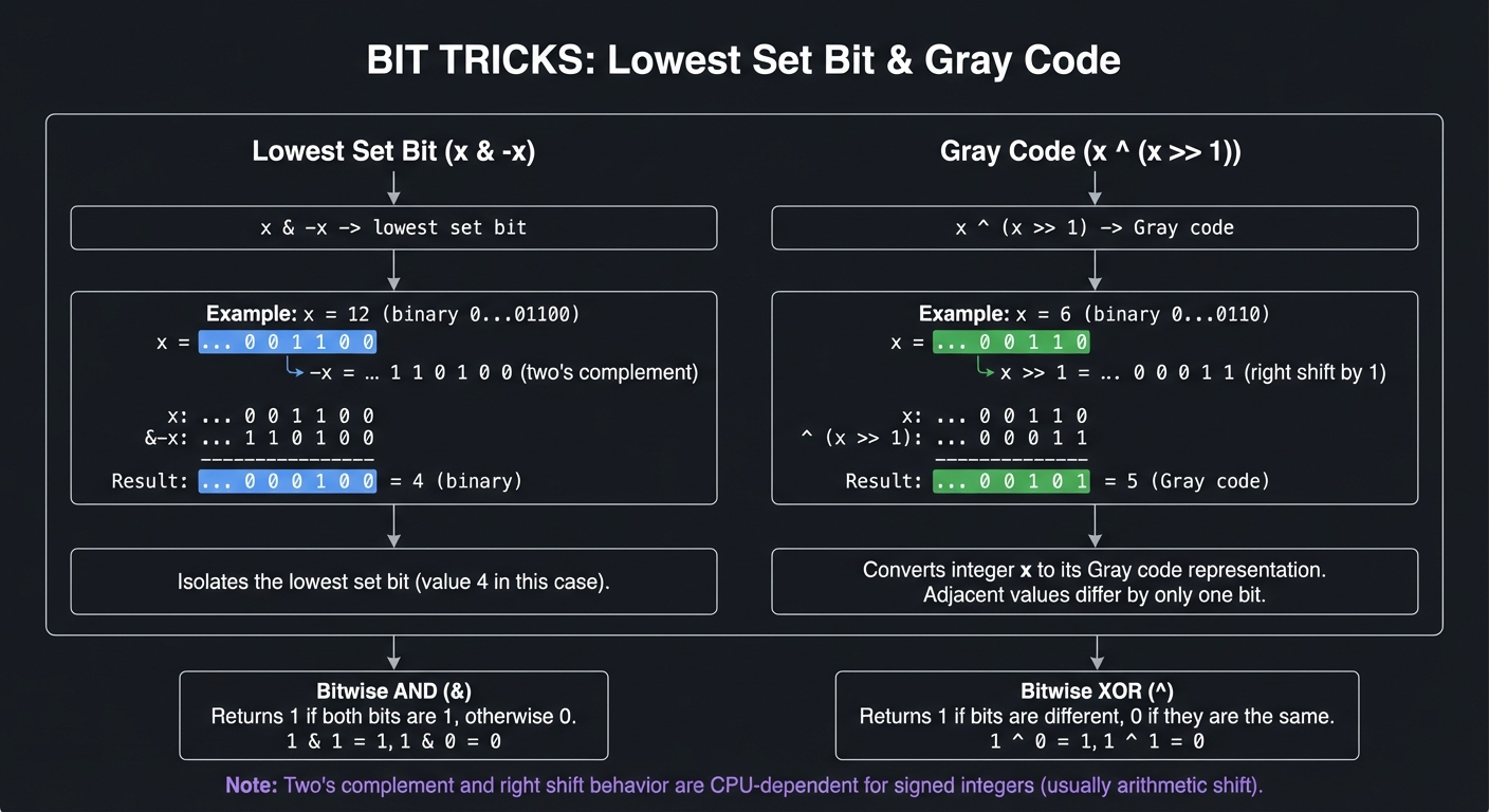
The Core Question You’re Answering

“How can you replace loops with constant-time bitwise transforms?”

Concepts You Must Understand First

Two’s complement and arithmetic shift behavior
Bit masks and shift boundaries
De Bruijn sequences for index lookup
Parallel prefix operations

Questions to Guide Your Design

How will you avoid undefined behavior in shifts?
Will you implement both 32-bit and 64-bit variants?
How will you benchmark fairly across methods?
Which operations benefit most from branch-free code?

Thinking Exercise

Compute popcount for 0b10110100 by hand and verify with each method.

The Interview Questions They’ll Ask

How do you isolate the lowest set bit?
What is Kernighan’s popcount trick?
How does De Bruijn indexing work?
Why do branch-free methods often run faster?

Hints in Layers

Hint 1: Implement Naive Versions First They become ground truth for later tests.

Hint 2: Add Kernighan and Parallel Methods Compare results and performance.

Hint 3: Add De Bruijn Indexing Use a precomputed table for bit positions.

Hint 4: Add Vectorized or Builtins Use compiler intrinsics when available.

Books That Will Help

Topic	Book	Chapter
Bitwise techniques	TAOCP Vol 4A	Ch. 7.1.3
Bit-level ops	CS:APP	Ch. 2
Low-level optimization	Write Great Code, Vol. 2	Ch. 6
Systems perspective	Inside the Machine	Ch. 4

Common Pitfalls & Debugging

Problem: “Results differ between 32-bit and 64-bit”

Why: Using incorrect masks or shift widths.
Fix: Define masks explicitly and use fixed-width types.
Quick test: Run the same input on both widths and compare.

Problem: “Shift by 64 causes crash”

Why: Shifting by word size is undefined in C.
Fix: Guard shift amounts or mask them.
Quick test: Add boundary tests for shift=0 and shift=63.

Implementation Hints:

Population count (multiple methods):

// Naive O(bits)
int popcount_naive(uint64_t x) {
    int count = 0;
    while (x) { count += x & 1; x >>= 1; }
    return count;
}

// Kernighan's trick O(set bits)
int popcount_kernighan(uint64_t x) {
    int count = 0;
    while (x) { x &= x - 1; count++; }  // Clears lowest set bit
    return count;
}

// Parallel bit count O(log bits)
int popcount_parallel(uint64_t x) {
    x = x - ((x >> 1) & 0x5555555555555555);
    x = (x & 0x3333333333333333) + ((x >> 2) & 0x3333333333333333);
    x = (x + (x >> 4)) & 0x0F0F0F0F0F0F0F0F;
    return (x * 0x0101010101010101) >> 56;
}

// Hardware (if available)
int popcount_hw(uint64_t x) {
    return __builtin_popcountll(x);
}

Lowest set bit:

int lowest_set_bit(uint64_t x) {
    // x & -x isolates lowest set bit
    return __builtin_ctzll(x);  // Count trailing zeros
}

// De Bruijn method (without hardware support)
static const int debruijn[64] = {...};
int lowest_set_debruijn(uint64_t x) {
    return debruijn[((x & -x) * 0x03f79d71b4cb0a89) >> 58];
}

Next permutation with same popcount:

// Generate next number with same number of set bits
uint64_t next_same_popcount(uint64_t x) {
    uint64_t smallest = x & -x;
    uint64_t ripple = x + smallest;
    uint64_t ones = x ^ ripple;
    ones = (ones >> 2) / smallest;
    return ripple | ones;
}
// 0b0011 → 0b0101 → 0b0110 → 0b1001 → 0b1010 → 0b1100

Learning milestones:

Popcount works all ways → You understand parallel reduction
Can find bit positions without loops → You understand De Bruijn
Next permutation works → You understand bit manipulation
Performance matches theory → You understand optimization

Definition of Done

Bit tricks match naive results for random inputs
De Bruijn indexing returns correct bit positions
32-bit and 64-bit variants both pass tests
Benchmarks show measurable speedups

CAPSTONE

Project 15: TAOCP Algorithm Visualization and Verification Suite

File: LEARN_TAOCP_DEEP_DIVE.md
Main Programming Language: C
Alternative Programming Languages: Rust, C++ with graphics
Coolness Level: Level 5: Pure Magic
Business Potential: 4. The “Open Core” Infrastructure
Difficulty: Level 5: Master
Knowledge Area: All of TAOCP
Software or Tool: Building: Algorithm Visualization Suite
Main Book: All TAOCP volumes

What you’ll build: An interactive suite that visualizes and verifies algorithms from all TAOCP volumes—allowing step-by-step execution, comparison of algorithms, and verification that your implementations match Knuth’s mathematical analysis.

Why this is the ultimate goal: This integrates everything you’ve learned. You’ll create a tool that helps others learn TAOCP, while deepening your own understanding. Building visualizations requires truly understanding algorithms; verification requires understanding their analysis.

Core challenges you’ll face:

Integrating all previous projects → maps to software architecture
Real-time visualization → maps to graphics programming
Step-by-step execution → maps to instrumentation
Statistical verification → maps to empirical testing

Difficulty: Master Time estimate: 2+ months Prerequisites:

Most previous projects completed
Graphics library familiarity (ncurses, SDL, or web)
Deep TAOCP knowledge

Real world outcome:

$ ./taocp_suite

Welcome to the TAOCP Algorithm Suite!
Covering Volumes 1-4B

Choose a topic:
1. Fundamental Algorithms (Vol 1)
2. Random Numbers & Arithmetic (Vol 2)
3. Sorting & Searching (Vol 3)
4. Combinatorial Algorithms (Vol 4)

> 3

Sorting & Searching Algorithms:
1. Comparison-based sorting
2. Distribution sorting
3. Search trees
4. Hashing

> 1

[Visualization window opens]

┌─ Quicksort vs Heapsort vs Mergesort ─────────────────────────┐
│                                                               │
│  ████                   █████                ██████           │
│  █████                  ██████               ███████          │
│  ██████   Quicksort    ███████   Heapsort   ████████ Merge   │
│  ███████                ████████             █████████        │
│  ████████               █████████            ██████████       │
│                                                               │
│  Comparisons: 15,234    Comparisons: 18,456  Comps: 16,007   │
│  Swaps: 4,567           Swaps: 12,345        Moves: 16,007   │
│  Theoretical: n log n = 16,610                               │
│                                                               │
│  [Step] [Run] [Reset] [Random Data] [Nearly Sorted]          │
└───────────────────────────────────────────────────────────────┘

> step
[Shows one comparison/swap at a time with highlighting]

> verify 10000
Running 10000 trials...
Algorithm   | Avg Comps  | Predicted  | Ratio
------------|------------|------------|------
Quicksort   | 1.386n lg n| 1.386n lg n| 1.002
Heapsort    | 2.0n lg n  | 2n lg n    | 0.998
Mergesort   | n lg n     | n lg n     | 1.001

All within 1% of Knuth's predictions!

Visual Model

Algorithm -> Instrumentation -> Logs -> Visualization -> Verification
    |              |             |          |              |
  core          counters       JSON     charts/steps     compare

taocp verification pipeline

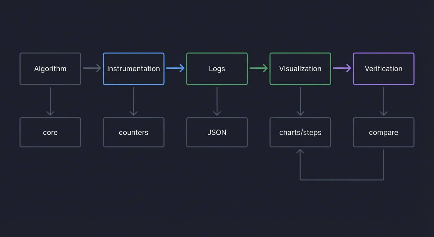
The Core Question You’re Answering

“How do you prove your implementations match Knuth’s analysis, and how do you make that proof visible to others?”

Concepts You Must Understand First

Instrumentation and deterministic replay
Benchmarking methodology and variance
Visualization pipelines (data -> view)
Integration testing across multiple modules

Questions to Guide Your Design

What is the plugin interface for adding new algorithms?
Which metrics are mandatory across all algorithms?
How will you avoid measurement bias (warm-up, cache effects)?
How will you store and replay experiment runs?

Thinking Exercise

Design a minimal metric schema (JSON) that records comparisons, swaps, time, and input size for any algorithm. What fields are required?

The Interview Questions They’ll Ask

How do you validate that an algorithm matches theoretical bounds?
How would you design a fair benchmark across multiple algorithms?
What architecture enables easy addition of new algorithms?
How do you ensure visualizations are truthful and not misleading?

Hints in Layers

Hint 1: Start With CLI Tracing Log every comparison/swap to a file and replay it.

Hint 2: Add a Unified Metrics API One interface for counters and timing across all modules.

Hint 3: Build a Simple Viewer Start with ASCII charts before adding graphics.

Hint 4: Add Verification Checks Compare measured ratios against expected formulas.

Books That Will Help

Topic	Book	Chapter
Algorithm analysis	TAOCP (all volumes)	Relevant sections
Performance measurement	The Pragmatic Programmer	Ch. 8
Systematic testing	Code Complete	Ch. 22
Experimental method	Algorithms, 4th Edition	Ch. 1.4

Common Pitfalls & Debugging

Problem: “Metrics vary wildly between runs”

Why: Uncontrolled input or system noise.
Fix: Fix random seeds and run multiple trials.
Quick test: Run 10 trials and compute mean and variance.

Problem: “Visualization disagrees with logs”

Why: Parsing errors or inconsistent schema.
Fix: Validate logs with a schema checker before rendering.
Quick test: Use a small input and manually verify a few steps.

Learning milestones:

All algorithms visualize correctly → You understand them deeply
Statistics match theory → You’ve verified TAOCP
Others can learn from your tool → You can teach
Code is clean and extensible → You’re a master programmer

Definition of Done

All modules integrate via a common metrics API
Logs replay deterministically to identical visuals
Measured ratios match theoretical predictions
At least one end-to-end demo runs cleanly

Project Comparison Table

#	Project	Volume	Difficulty	Time	Understanding
1	MMIX Simulator	1	Expert	3-4 weeks	⭐⭐⭐⭐⭐
2	Mathematical Toolkit	1	Intermediate	1-2 weeks	⭐⭐⭐⭐
3	Data Structures Library	1	Intermediate	2 weeks	⭐⭐⭐⭐
4	Tree Algorithms	1	Advanced	2 weeks	⭐⭐⭐⭐
5	Random Number Suite	2	Advanced	2-3 weeks	⭐⭐⭐⭐⭐
6	Arbitrary Precision	2	Expert	3-4 weeks	⭐⭐⭐⭐⭐
7	Floating-Point Emulator	2	Expert	2 weeks	⭐⭐⭐⭐
8	Sorting Collection	3	Advanced	2-3 weeks	⭐⭐⭐⭐
9	Search Trees	3	Expert	3-4 weeks	⭐⭐⭐⭐⭐
10	Hash Tables	3	Advanced	2 weeks	⭐⭐⭐⭐
11	Combinatorial Generator	4A	Advanced	2 weeks	⭐⭐⭐⭐
12	DLX + SAT Solver	4B	Master	4-6 weeks	⭐⭐⭐⭐⭐
13	BDD Analyzer	4A	Expert	2-3 weeks	⭐⭐⭐⭐⭐
14	Bitwise Magic	4A	Intermediate	1 week	⭐⭐⭐
15	Visualization Suite	All	Master	2+ months	⭐⭐⭐⭐⭐

Recommended Learning Path

Year 1: Fundamentals (Volume 1 + Basics)

Project 2: Mathematical Toolkit (1-2 weeks)
Project 3: Data Structures Library (2 weeks)
Project 4: Tree Algorithms (2 weeks)
Project 1: MMIX Simulator (3-4 weeks) - can skip but highly recommended

Year 2: Numbers and Arithmetic (Volume 2)

Project 5: Random Number Suite (2-3 weeks)
Project 6: Arbitrary Precision Arithmetic (3-4 weeks)
Project 7: Floating-Point Emulator (2 weeks)

Year 3: Sorting and Searching (Volume 3)

Project 8: Complete Sorting Collection (2-3 weeks)
Project 10: Hash Table Laboratory (2 weeks)
Project 9: Search Tree Collection (3-4 weeks)

Year 4: Combinatorics (Volume 4)

Project 14: Bitwise Magic Toolkit (1 week)
Project 11: Combinatorial Object Generator (2 weeks)
Project 13: Boolean Function Analyzer (2-3 weeks)
Project 12: Dancing Links + SAT Solver (4-6 weeks)

Final: Integration

Project 15: TAOCP Visualization Suite (2+ months)

Summary

#	Project Name	Main Language	TAOCP Coverage
1	MMIX Simulator	C	Vol 1: Machine Architecture
2	Mathematical Toolkit	C	Vol 1: Chapter 1 (Foundations)
3	Data Structures Library	C	Vol 1: Section 2.2 (Lists)
4	Tree Algorithms	C	Vol 1: Section 2.3 (Trees)
5	Random Number Suite	C	Vol 2: Chapter 3 (Random)
6	Arbitrary Precision	C	Vol 2: Section 4.3 (Arithmetic)
7	Floating-Point Emulator	C	Vol 2: Section 4.2 (Float)
8	Sorting Collection	C	Vol 3: Chapter 5 (Sorting)
9	Search Trees	C	Vol 3: Section 6.2 (Trees)
10	Hash Tables	C	Vol 3: Section 6.4 (Hashing)
11	Combinatorial Generator	C	Vol 4A: Section 7.2.1
12	DLX + SAT Solver	C	Vol 4B: Section 7.2.2
13	BDD Analyzer	C	Vol 4A: Section 7.1.4
14	Bitwise Magic	C	Vol 4A: Section 7.1.3
15	Visualization Suite	C	All Volumes

Key Resources

The Books Themselves

“The Art of Computer Programming, Volume 1: Fundamental Algorithms” (3rd ed, 1997)
“The Art of Computer Programming, Volume 2: Seminumerical Algorithms” (3rd ed, 1998)
“The Art of Computer Programming, Volume 3: Sorting and Searching” (2nd ed, 1998)
“The Art of Computer Programming, Volume 4A: Combinatorial Algorithms, Part 1” (2011)
“The Art of Computer Programming, Volume 4B: Combinatorial Algorithms, Part 2” (2022)
“The MMIX Supplement” by Martin Ruckert - Translations of algorithms to MMIX

Online Resources

Knuth’s TAOCP Page - Official site with errata
TAOCP Solutions - Community solutions
MMIX Simulator - Official MMIX tools
Dancing Links Paper - Knuth’s original paper

Companion Books (from your collection)

“Concrete Mathematics” by Graham, Knuth, Patashnik - Mathematical foundations
“Introduction to Algorithms” (CLRS) - Modern algorithm perspective
“Computer Organization and Design” by Patterson & Hennessy - For MMIX understanding
“Algorithms, Fourth Edition” by Sedgewick & Wayne - Java perspective on same topics

You’re embarking on one of the greatest intellectual journeys in computer science. TAOCP has shaped the field for 60 years. By working through these projects, you’ll understand computing at the deepest level—the level that Knuth himself operates at. Start with Project 2 (Mathematical Toolkit) and work your way through. Welcome to the Art.