Quantum Algorithms - From Zero to Quantum Master
Goal: Deeply understand how quantum mechanics revolutionizes computation. You will move from classical bits to qubits, mastering the mathematics of superposition and entanglement. By building simulations and implementing real quantum circuits (Shor’s, Grover’s, VQE), you will internalize the “Quantum Advantage”—learning exactly when quantum wins, why it breaks current cryptography, and how “quantum-inspired” classical code can solve today’s problems.
Why Quantum Algorithms Matter
In 1981, Richard Feynman observed that simulating nature on a classical computer is fundamentally inefficient because nature isn’t classical—it’s quantum. This observation launched a new era of computing.
The Exponential Wall
A classical computer with $N$ bits can represent one of $2^N$ states at a time. A quantum computer with $N$ qubits can exist in a superposition of all $2^N$ states simultaneously.
Number of Qubits (N) | Classical States Represented | Quantum States Represented (Simultaneously)
---------------------|------------------------------|---------------------------------------------
1                    | 1                            | 2
10                   | 1                            | 1,024
20                   | 1                            | 1,048,576
50                   | 1                            | 1.12 Quadrillion
300                  | 1                            | More than atoms in the observable universe
The Real-World Impact
- Shor’s Algorithm: Makes the core of our digital security (RSA) obsolete by factoring numbers in polynomial time instead of sub-exponential time.
- Grover’s Algorithm: Searches unstructured data with a quadratic speedup ($O(\sqrt{N})$).
- VQE (Variational Quantum Eigensolver): Allows us to simulate molecules for drug discovery and material science that are impossible to simulate classically.
The Qubit and the Bloch Sphere
Unlike a classical bit (0 or 1), a qubit is a state vector in a 2D complex Hilbert space. We visualize it using the Bloch Sphere.
          |0⟩ (North Pole: Z=1)
            |
            |   .  (θ, φ)
            |  /
            | /
            |/____ (Y axis)
           /
          / (X axis)
         /
        |1⟩ (South Pole: Z=-1)
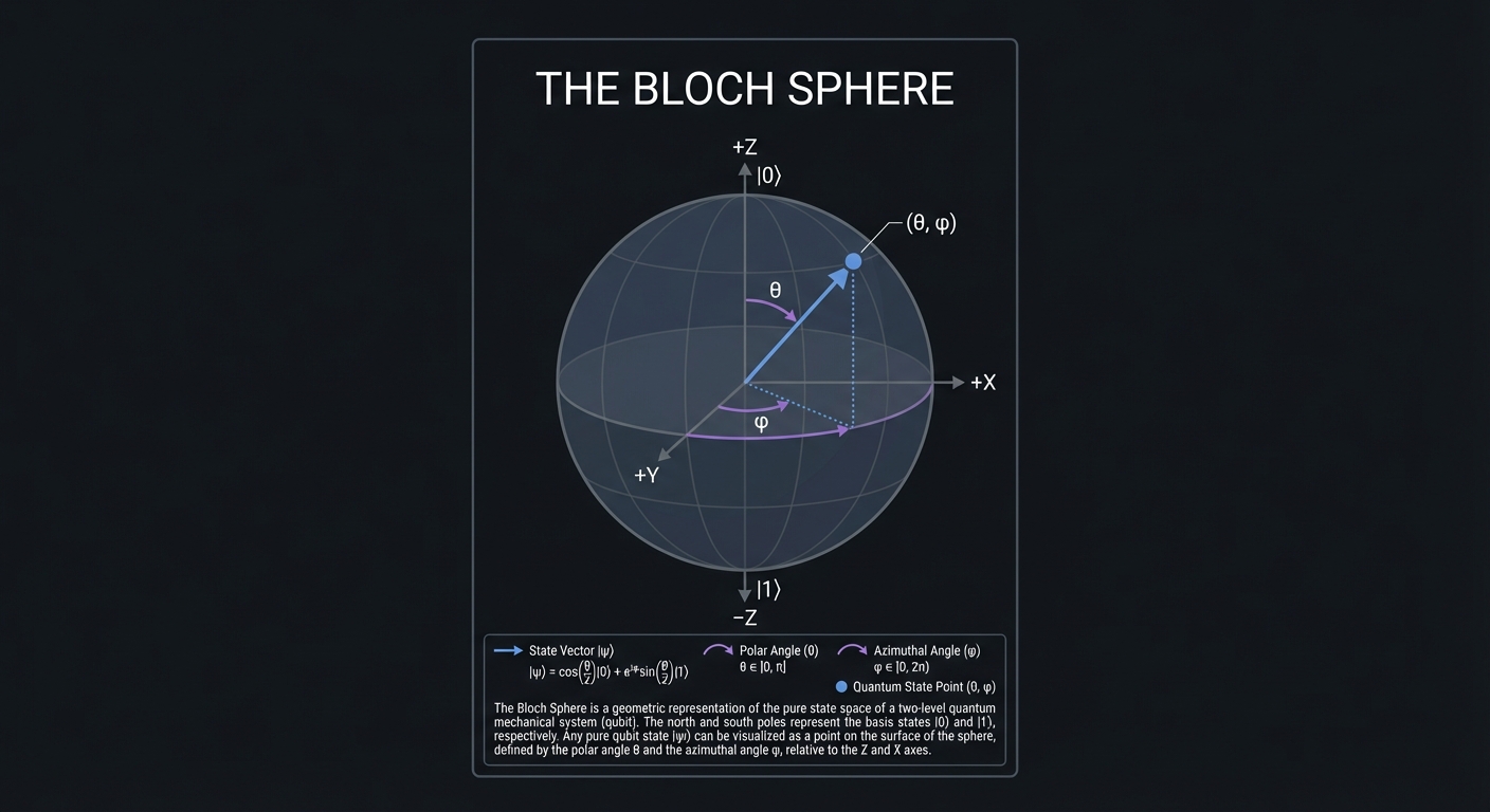
| Any single-qubit operation is just a rotation on this sphere. If you apply a Hadamard gate (H), you rotate the qubit from $ | 0\rangle$ or $ | 1\rangle$ to the equator, creating a superposition. |
Recommended Reading: “Quantum Computation and Quantum Information” (Nielsen & Chuang) - Ch 1.2
Superposition: The Parallelism of State
Superposition is a linear combination of basis states.
Classical: [ 0 ] or [ 1 ] (Deterministic switch)

Quantum:   α|0⟩ + β|1⟩   (Probabilistic wave)
           where |α|² + |β|² = 1
When you have $n$ qubits, the state space is $2^n$ dimensional. A quantum algorithm manipulates this massive space using interference.
Entanglement: Spooky Correlation
Entanglement allows qubits to be linked such that their states cannot be described independently.
       Alice's Qubit          Bob's Qubit
      ┌─────────────┐        ┌─────────────┐
      │     [H]      │        │             │
      │      |       │        │             │
      │    [●]───────┼────────┼───[X]       │
      └──────│──────┘        └──────│──────┘
             └──────────────────────┘
                 Shared Correlation
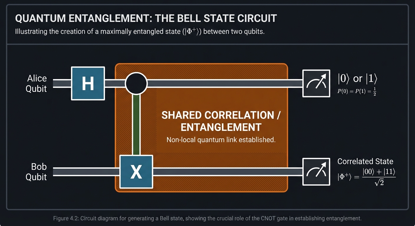
| If these qubits are entangled in the $ | \Phi^+ \rangle = \frac{1}{\sqrt{2}}( | 00\rangle + | 11\rangle)$ state, measuring Alice’s qubit and getting 1 means Bob’s qubit instantly becomes 1, regardless of distance. |
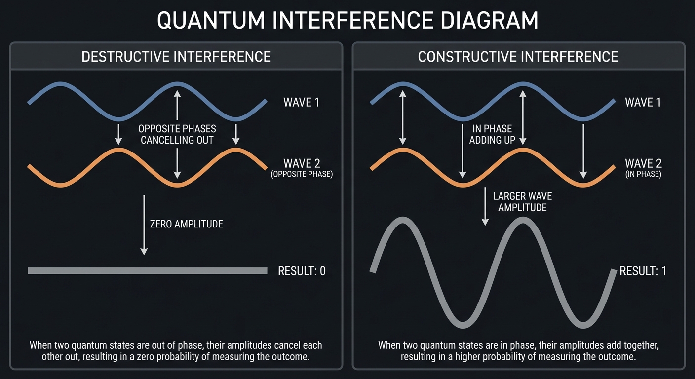
Quantum Interference
This is the “magic” that makes quantum algorithms work. We don’t just “try every path.” We use gates to make paths that lead to the wrong answer cancel each other out (destructive interference) and paths that lead to the correct answer reinforce each other (constructive interference).
Wrong Paths (Probabilities cancel)      Correct Path (Probabilities add up)
       _/\_                                     /\
      /    \                                   /  \
     /      \                                 /    \
     \_    _/                                /      \
       \  /                                 /        \
       \/                                  ----------
   Result: 0                                Result: 1
Quantum Oracles and Phase Kickback
An Oracle is a “black box” that marks the solution to a problem. It doesn’t find the answer; it recognizes it.
Input |x⟩ ────[ Oracle ]──── (-1)^f(x) |x⟩
Phase Kickback is a technique where the result of an operation on an auxiliary qubit is “kicked back” into the phase of the main register. This is how Grover’s algorithm flips the sign of the correct answer.
Recommended Reading: “Quantum Computing for Computer Scientists” (Yanofsky & Mannucci) - Ch 6
Quantum Fourier Transform (QFT)
The QFT is the quantum analogue of the Discrete Fourier Transform. It maps a state from the computational basis to the Fourier basis. It’s the engine behind Shor’s algorithm, allowing us to find the period of a function exponentially fast.
|j⟩ ────[ QFT ]──── 1/√N ∑ exp(2πijk/N) |k⟩
While the classical FFT takes $O(N \log N)$ steps, the QFT takes only $O((\log N)^2)$ gates.
Variational Quantum Eigensolver (VQE) Logic
VQE is a hybrid algorithm designed for the NISQ (Noisy Intermediate-Scale Quantum) era. It uses a classical optimizer to minimize the energy of a quantum wavefunction.
┌────────────────┐      ┌─────────────────┐      ┌────────────────┐
│ Quantum Device │ ───> │ Measure Energy  │ ───> │ Classical Opt  │
└───────▲────────┘      └─────────────────┘      └───────┬────────┘
        │                                                │
        └───────────────── Update Parameters <───────────┘
Recommended Reading: “Quantum Computing in Action” (Johan Vos) - Ch 8
Quantum Machine Learning & Hilbert Spaces
QML leverages the fact that $N$ qubits define a $2^N$ dimensional Hilbert space. Mapping classical data into this space (Feature Mapping) can make non-linearly separable data easy to classify.
Data (R^2) ───[ Feature Map ]───> Quantum State (H^2^n)
   (x, y)                         |ψ(x,y)⟩
Post-Quantum Cryptography & Lattices
As quantum computers threaten RSA and ECC, we need “quantum-resistant” math. Lattice-based cryptography relies on the hardness of the Shortest Vector Problem (SVP), which currently has no known efficient quantum solution.
Lattice Λ = { ∑ a_i v_i }
Objective: Find the shortest non-zero vector in Λ.
Concept Summary Table
| Concept Cluster | What You Need to Internalize | ||
|---|---|---|---|
| Linear Algebra Engine | Quantum computing is matrix multiplication on complex vectors. No magic, just math. | ||
| Bloch Sphere & Rotations | Qubits are vectors; gates are rotations. Visualizing this is key to intuition. | ||
| Superposition & Measurement | You can exist in many states, but looking at it forces a choice. Probability is $ | \text{amplitude} | ^2$. |
| Entanglement | Non-classical correlation. The basis for teleportation and superdense coding. | ||
| Oracles & Marking | How to “tag” an answer using phase flips without knowing what the answer is. | ||
| QFT & Phase Estimation | The engine of speedups. Finding periodicities in data exponentially fast. | ||
| Hybrid Computing (VQE/QAOA) | Using a classical optimizer to “tune” a noisy quantum computer. | ||
| Post-Quantum Math | Lattice-based problems that even quantum computers find difficult to solve. |
Deep Dive Reading by Concept
Foundations & Linear Algebra
| Concept | Book & Chapter | |———|—————-| | Linear Algebra for Quantum | “Quantum Computation and Quantum Information” by Nielsen & Chuang — Ch. 2 | | Complex Vector Spaces | “Quantum Computing for Computer Scientists” by Yanofsky & Mannucci — Ch. 2 | | The Bloch Sphere | “Quantum Computing: An Applied Approach” by Jack Hidary — Ch. 1 |
Quantum Mechanics & Circuits
| Concept | Book & Chapter | |———|—————-| | Postulates of QM | “Quantum Computation and Quantum Information” — Ch. 2.2 | | Universal Gate Sets | “Quantum Computing: An Applied Approach” — Ch. 3 | | Entanglement & Bell States | “Computer Science From Scratch” by David Kopec — Ch. 12 |
Algorithms & Hybrid Systems
| Concept | Book & Chapter | |———|—————-| | Grover’s Search | “Quantum Computer Science” by David Mermin — Ch. 4 | | Shor’s Factoring | “Quantum Computation and Quantum Information” — Ch. 5.3 | | VQE & Hybrid Algos | “Quantum Computing in Action” by Johan Vos — Ch. 8 | | QAOA & Optimization | “Quantum Computing: An Applied Approach” — Ch. 7 |
Advanced Topics
| Concept | Book & Chapter | |———|—————-| | QML & Feature Spaces | “Quantum Computing: An Applied Approach” — Ch. 9 | | Post-Quantum Math | “Serious Cryptography” — Ch. 12 | | Lattice-Based Crypto | “An Introduction to Mathematical Cryptography” — Ch. 7 | | Error Mitigation | “Quantum Computing in Action” — Ch. 10 |
Project 1: The Linear Algebra “Engine” (Classical Simulation)
- Main Programming Language: Python (NumPy)
- Alternative Programming Languages: C++, Rust, Julia
- Difficulty: Level 3: Advanced
- Knowledge Area: Linear Algebra / Simulation
What you’ll build: A classical simulator that represents qubits as vectors and quantum gates as matrices. You will implement the Tensor Product to handle multi-qubit systems and simulate state evolution through matrix multiplication.
Why it teaches Quantum: Before using a library like Qiskit, you must understand that quantum computing is just “Linear Algebra on steroids.” This project forces you to realize that 2 qubits is a 4-element vector, and 10 qubits is a 1024-element vector—explaining why classical computers struggle as qubit counts grow.
Real World Outcome
You will have a robust Python library (engine.py) that functions like a “Mini-Qiskit”. You will be able to construct any quantum circuit by hand-calculating Kronecker products and performing state vector updates.
When you run your engine, you will see a step-by-step trace of the probability amplitudes as they shift through the complex plane.
Example Usage:
from engine import Simulator, gates
import numpy as np

# Initialize a 2-qubit system in state |00>
sim = Simulator(num_qubits=2)

# Apply a Hadamard gate to the first qubit to create superposition
# This expands the 2x2 H matrix into a 4x4 matrix using I ⊗ H
sim.apply(gates.H, target=0)

# Apply a CNOT gate to entangle them
# Target is q1, Control is q0
sim.apply(gates.CNOT, control=0, target=1)

print(f"Final State Vector: {sim.get_state()}")
print(f"Measurement Sample: {sim.measure()}")
Example Output:
$ python run_sim.py
[INFO] Initializing 2 qubits. State vector size: 4
[STEP 1] Applying H gate to qubit 0...
         New State: [0.707+0.j, 0.707+0.j, 0.000+0.j, 0.000+0.j]
[STEP 2] Applying CNOT (C:0, T:1)...
         New State: [0.707+0.j, 0.000+0.j, 0.000+0.j, 0.707+0.j]
[RESULT] Execution complete.
         Final Vector: [0.7071+0j, 0j, 0j, 0.7071+0j]
         Probabilities: {'00': 0.5, '11': 0.5}
         Single Measurement Outcome: '11'
# You have successfully simulated an entangled Bell State!
The Core Question You’re Answering
“Why can’t my laptop simulate 50 qubits if it’s just ‘linear algebra’?”
Before you write any code, calculate the memory required to store a state vector for 50 qubits using 128-bit complex numbers. (Hint: $2^{50} \times 16$ bytes). You’ll quickly see why the “Quantum Advantage” exists—classical memory requirements grow exponentially.
Concepts You Must Understand First
- Complex Vector Spaces
- What is a Hilbert Space?
- How do you calculate the norm of a complex vector?
- Tensor Products (Kronecker Product)
- If I have a matrix A (2x2) and B (2x2), what is the size of $A \otimes B$?
- How do you apply a gate to only the second qubit in a 3-qubit system using $I \otimes U \otimes I$?
- Unitary Matrices
- Why must gates be unitary ($U^\dagger U = I$)?
- How does this relate to the conservation of probability?
Questions to Guide Your Design
- Memory Management
- How will you store the state vector efficiently?
- At what number of qubits does your simulation start to crawl?
- Gate Lifting
- If you have a 3-qubit system and want to apply a Hadamard gate to qubit 1, how do you construct the $8 \times 8$ matrix from the $2 \times 2$ H gate?
- Measurement Collapse
- After measuring a qubit and getting a result (say
0), how do you update the state vector so that subsequent measurements are consistent?
- After measuring a qubit and getting a result (say
Thinking Exercise
The CNOT Matrix
Trace the CNOT operation on the basis states:
-
$ 00\rangle \to 00\rangle$ -
$ 01\rangle \to 01\rangle$ -
$ 10\rangle \to 11\rangle$ -
$ 11\rangle \to 10\rangle$
Now, write down the 4x4 matrix that performs this mapping. Notice how it swaps the “amplitudes” of the target qubit only when the control qubit is 1.
The Interview Questions They’ll Ask
- “How does the size of the state vector scale with the number of qubits?”
- “Why is a quantum state vector always normalized to 1?”
- “What is the difference between a sparse and a dense matrix in the context of quantum simulation?”
- “Why is it computationally expensive to simulate entanglement classically?”
- “If a gate is not unitary, what happens to the total probability of the system?”
Hints in Layers
Hint 1: Start with 1 Qubit
Represent the state as np.array([1, 0], dtype=complex). Define H as np.array([[1, 1], [1, -1]]) / np.sqrt(2).
Hint 2: Multi-qubit Tensor
Use np.kron(A, B) to compute the Kronecker product. To apply a gate $U$ to qubit $k$ of $n$:
$Op = I \otimes I \otimes \dots \otimes U \otimes \dots \otimes I$ (where $U$ is at position $k$).
Hint 3: Measurement To measure, generate a random number $r \in [0, 1]$. Sum the squared magnitudes of the amplitudes until you reach $r$. That index is your measurement outcome.
Books That Will Help
| Topic | Book | Chapter |
|---|---|---|
| Linear Algebra Foundations | “Quantum Computation and Quantum Information” | Ch. 2.1 |
| Gate Matrices & Qubits | “Quantum Computing: An Applied Approach” | Ch. 2 |
| Python Simulation Basics | “Computer Science From Scratch” | Ch. 12 |
Project 2: “Hello Quantum” (Framework Basics)
- Main Programming Language: Python (Qiskit)
- Alternative Programming Languages: Cirq, Q#
- Difficulty: Level 1: Beginner
- Knowledge Area: Quantum Circuit Design
What you’ll build: A series of scripts that implement the “Hello World” of quantum: Creating a Bell State, performing a swap test, and running a circuit on a real IBM Quantum backend (via the cloud).
Why it teaches Quantum: It moves you from “manual matrix math” to using industry-standard abstractions. You’ll learn about “Transpilation”—how your high-level gates are broken down into the native gates of a physical quantum processor.
Real World Outcome
You will have a collection of .py files or Jupyter notebooks that generate circuit diagrams and execute them on both local simulators and remote quantum hardware.
Example Code:
from qiskit import QuantumCircuit, transpile
from qiskit_aer import AerSimulator
from qiskit.visualization import plot_histogram

qc = QuantumCircuit(2)
qc.h(0)
qc.cx(0, 1) # Bell State
qc.measure_all()

simulator = AerSimulator()
result = simulator.run(qc).result()
counts = result.get_counts()
print(counts) # Output: {'00': 512, '11': 512} (approx)
What you will see:
- A visual circuit diagram with wires and boxes.
- A histogram showing a 50/50 split between
00and11, proving the qubits are perfectly correlated.
The Core Question You’re Answering
“How do I take a mathematical idea and run it on a physical device I don’t own?”
Concepts You Must Understand First
- Circuits as ‘Scores’
- Why do we read circuits from left to right?
- What is the difference between a “Quantum Register” and a “Classical Register”?
- The Transpiler
- If a physical chip only supports
CNOTandRzgates, how does it run yourHadamardgate?
- If a physical chip only supports
- Shots vs. Probability
- Why do we need to run a circuit 1024 times (shots) to see the probability?
Questions to Guide Your Design
- Backend Selection
- When should you use a “Statevector Simulator” vs a “Qasm Simulator”?
- Noise Modeling
- How can you simulate the errors of a real IBM chip on your local machine?
- Optimization
- How many gates can you add before the “noise” makes the result useless?
Thinking Exercise
The Probabilistic Nature
If you run a circuit that results in the state $\frac{1}{\sqrt{2}}(|0\rangle + |1\rangle)$ just once, what do you get? If you run it 1000 times, what do you get? How does this relate to the law of large numbers?
The Interview Questions They’ll Ask
- “What is Qiskit and why is it used?”
- “What does it mean to ‘transpile’ a circuit?”
- “Explain the difference between a simulator and a real QPUs (Quantum Processing Units).”
- “Why is measurement a destructive process in quantum computing?”
Hints in Layers
Hint 1: Circuit Setup
qc = QuantumCircuit(n_qubits, n_bits) is your starting point.
Hint 2: Visualization
Use qc.draw('mpl') in a notebook to see the beautiful diagram.
Hint 3: Real Hardware
You’ll need an IBM Quantum API key. Use QiskitRuntimeService to find the least busy backend.
Books That Will Help
| Topic | Book | Chapter |
|---|---|---|
| Qiskit Basics | “Quantum Computing in Action” | Ch. 2-3 |
| Framework Overviews | “Quantum Computing: An Applied Approach” | Ch. 11 |
| Applied Quantum Algos | “Dancing with Qubits” | Ch. 9 |
Project 3: The Quantum Bridge (Teleportation)
- Main Programming Language: Python (Qiskit)
- Alternative Programming Languages: Cirq
- Difficulty: Level 2: Intermediate
- Knowledge Area: Quantum Communication Protocols
What you’ll build: An implementation of the Quantum Teleportation protocol. You will “teleport” an unknown qubit state from Alice to Bob using a shared entangled pair and two bits of classical information.
Why it teaches Quantum: It’s the ultimate test of understanding entanglement and the “No-Cloning Theorem.” You cannot copy a qubit, but you can move its information.
Real World Outcome
You will create a protocol where a qubit’s state is transferred across a system without the physical qubit moving. You’ll verify this by performing “State Tomography” or simply by checking that Bob’s measurement results match Alice’s initial state preparation.
Example Script Output:
$ python teleport.py --state "0.6|0> + 0.8|1>"
[INIT] Alice prepares secret state: 0.6|0> + 0.8|1> (Ry(1.85 rad))
[STEP 1] Generating entangled pair (EPR pair) between Alice and Bob...
[STEP 2] Alice performs Bell Basis measurement on her two qubits...
         Results: cr0=1, cr1=0
[STEP 3] Alice sends [1, 0] to Bob via classical channel...
[STEP 4] Bob applies Z-correction because cr0=1...
[VERIFY] Bob's qubit state: 0.600|0> + 0.800|1>
SUCCESS: Fidelity = 1.000. The state was teleported perfectly!
The Core Question You’re Answering
“If I teleport a qubit, is the information moving faster than light?”
Think about the two classical bits Alice has to send to Bob. Can Bob reconstruct the state before he gets those bits? This project proves that while entanglement is “instant,” information transfer is limited by the speed of light.
Concepts You Must Understand First
- The No-Cloning Theorem
- Why is it impossible to create an identical copy of an unknown quantum state?
- Book Reference: “Quantum Computation and Quantum Information” Ch 12.1
- Bell Basis Measurement
- How do you project two qubits into the Bell Basis using a CNOT and a Hadamard?
- Deferred Measurement Principle
- Why can we measure Alice’s qubits and then apply classical corrections to Bob’s?
Questions to Guide Your Design
- Protocol Steps
- Step 1: Entangle Qubit 1 and Qubit 2 (The shared resource).
- Step 2: Alice interacts her unknown Qubit 0 with her half of the entangled pair (Qubit 1).
- Step 3: Alice measures her two qubits.
- Step 4: Bob applies X or Z gates based on Alice’s results.
- Verification
- How do you verify Bob has the state if you can’t “look” at it without destroying it? (Hint: Perform a state tomography or run the inverse of Alice’s preparation).
Thinking Exercise
The Logic of Correction
If Alice measures 11, why does Bob need to apply both an X and a Z gate? Trace the state vector through the measurement and see how Bob’s qubit is “rotated” away from the target state by Alice’s measurement.
The Interview Questions They’ll Ask
- “Does quantum teleportation violate the speed of light?”
- “Explain the role of the shared entangled pair in the protocol.”
- “Why can’t we use teleportation to send classical bits faster than light?”
- “What happens to Alice’s original qubit after the teleportation?”
Hints in Layers
Hint 1: The Entangled Pair
Qubit 1 (Alice) and Qubit 2 (Bob) must be in the state $| \Phi^+ \rangle$. qc.h(1); qc.cx(1, 2).
Hint 2: Alice’s Part
Alice interacts her qubit 0 with qubit 1: qc.cx(0, 1); qc.h(0).
Hint 3: Classical Conditioning
Use qc.measure(0, cr0); qc.measure(1, cr1) and then qc.x(2).c_if(cr1, 1); qc.z(2).c_if(cr0, 1).
Books That Will Help
| Topic | Book | Chapter |
|---|---|---|
| Teleportation Logic | “Quantum Computation and Quantum Information” | Ch. 1.3.7 |
| Communication Protocols | “Quantum Computing: An Applied Approach” | Ch. 4 |
| Circuit Implementation | “Quantum Computing in Action” | Ch. 5 |
Project 4: Grover’s Search (The “Needle in a Haystack”)
- Main Programming Language: Python (Qiskit)
- Alternative Programming Languages: Cirq, Q#
- Difficulty: Level 3: Advanced
- Knowledge Area: Search Algorithms / Oracle Design
What you’ll build: A program that searches for a specific 3-bit or 4-bit “secret key” in an unstructured database using Grover’s Algorithm. You will design the Oracle and the Diffuser (Inversion about the Mean).
Why it teaches Quantum: It demonstrates “Amplitude Amplification.” You’ll see how the Oracle marks the answer with a negative phase, and how the Diffuser “boosts” that state while suppressing others.
Real World Outcome
You will see a probability distribution where the correct answer’s probability is nearly 100%, while others are suppressed. You will be able to search $N$ items in $\approx \sqrt{N}$ steps.
Example Output:
$ python grover.py --target "101"
[INIT] Database size: 8 items (3 qubits).
[STEP] Building Oracle for target '101'...
[STEP] Applying 2 Grover iterations...
[RUN] Executing on AerSimulator (1024 shots)...
Results:
  '101': 982  (Probability: 95.9%)
  '000': 6
  '011': 7
  ...
[SUCCESS] Target '101' found in 2 steps. Classical would take ~4-8.
The Core Question You’re Answering
“If I have $N$ items, why is $\sqrt{N}$ the magic number for searching them?”
Classical search is $O(N)$ because you check one by one. Grover’s uses rotations in Hilbert space. Imagine a vector pointing at “average.” Every Grover step rotates that vector toward the “answer.” If you rotate too many times, you’ll pass the answer and start pointing away again!
Concepts You Must Understand First
- Reflection Operators
- How do you reflect a vector across a plane in 2D?
- Oracle Marking (Phase Kickback)
-
Why does flipping the sign of a state ($ x\rangle \to - x\rangle$) “mark” it? - How do you use an ancillary qubit and a CNOT to achieve this?
-
- Geometric Interpretation
- How can Grover’s be viewed as a rotation between the “average” state and the “target” state?
Questions to Guide Your Design
- Oracle Scalability
- How do you build an Oracle for 4 qubits without manually writing every gate? (Hint: Use Multi-Controlled gates).
- Optimal Iterations
- What happens if you run 10 iterations on a 3-qubit system (8 states)? Why does the accuracy drop? (Hint: Over-rotation).
Thinking Exercise
The Diffuser Step
The diffuser is defined as $H^{\otimes n} (2|0\rangle\langle 0| - I) H^{\otimes n}$.
-
Trace what happens to the state $ 00\rangle$ through this operation. - Why do we need the Hadamards on both sides of the “Reflect about zero” operation? (Hint: Change of basis).
The Interview Questions They’ll Ask
- “What is the computational complexity of Grover’s algorithm vs classical search?”
- “Explain the ‘Inversion about the Mean’ conceptually.”
- “Can Grover’s algorithm be used to break AES? If so, how?”
- “Why is the number of iterations approximately $\frac{\pi}{4}\sqrt{N}$?”
Hints in Layers
Hint 1: The Oracle
For a target “101”, your oracle should flip the phase only if $q_0=1, q_1=0, q_2=1$. You can use qc.x(1) before and after a Multi-Controlled Z gate to make $q_1$ “appear” as a 1 to the gate.
Hint 2: Phase Kickback Use an auxiliary qubit in the $|-\rangle$ state. Apply a Multi-Controlled NOT (Toffoli) to this qubit. The state will pick up a $(-1)$ phase.
Hint 3: The Diffuser The core of the diffuser is a gate that flips the sign of every state except $|00…0\rangle$. This is often called the “Zero-Phase Oracle.”
Books That Will Help
| Topic | Book | Chapter |
|---|---|---|
| Algorithm Mechanics | “Quantum Computer Science” | Ch. 4 |
| Amplitude Amplification | “Quantum Computation and Quantum Information” | Ch. 6.1 |
| Oracle Design | “Quantum Computing for Computer Scientists” | Ch. 7 |
Project 5: Shor’s Algorithm (The RSA Breaker)
- Main Programming Language: Python (Qiskit)
- Alternative Programming Languages: Julia
- Difficulty: Level 5: Master
- Knowledge Area: Cryptography / Number Theory
What you’ll build: A “mini-Shor’s” that factors the number 15 or 21. You will implement the Order Finding subroutine using Quantum Phase Estimation (QPE) and the Quantum Fourier Transform (QFT).
Why it teaches Quantum: This is the “Holy Grail.” It combines modular exponentiation, QPE, and QFT to solve a problem classical computers find hard. You’ll learn how quantum computers find the periodicity of a mathematical function.
Real World Outcome
You will have a program that cracks small RSA-like public keys by finding the prime factors of a composite number $N$ using the quantum period-finding advantage.
Example Script Output:
$ python shors.py --N 21
[SETUP] Factoring N=21. Choosing random a=2.
[QUANTUM] Executing Quantum Phase Estimation on U_a...
[MEASURE] Result: Phase = 0.1666... (1/6)
[MATH] Denominator of phase is r=6.
[FACTOR] Period r=6 is even. Calculating gcd(a^(r/2) ± 1, N)...
         gcd(2^3 - 1, 21) = gcd(7, 21) = 7
         gcd(2^3 + 1, 21) = gcd(9, 21) = 3
[SUCCESS] Factors of 21 are 3 and 7.
# Total Quantum Gates used: 450
The Core Question You’re Answering
“Why does finding the ‘period’ of a function allow me to break encryption?”
Shor’s algorithm doesn’t “guess” the factors. It converts the factoring problem into a period-finding problem. Because quantum computers can find the period of $f(x) = a^x \mod N$ exponentially faster than classical ones using QFT, the entire security of the modern world shifts.
Concepts You Must Understand First
- Modular Arithmetic
- What is the “period” of $a^x \mod N$?
- Why is finding this period equivalent to factoring $N$?
- Quantum Fourier Transform (QFT)
- How does the QFT transform a time-domain signal (amplitudes) into frequency-domain information?
- Book Reference: “The C Programming Language” (Wait, wrong book) -> “Quantum Computation and Quantum Information” Ch 5.1
- Quantum Phase Estimation (QPE)
- How do you use an oracle $U$ to write its phase $\phi$ into the register qubits?
Questions to Guide Your Design
- Circuit Complexity
- How many qubits do you need to factor $N=15$? (Hint: Register qubits for $N$ plus precision qubits for the phase).
- Hardcoding Oracles
- Since building a general modular exponentiation circuit is very hard, how can you “hardcode” the $(7^x \mod 15)$ operation using CNOTs and Swaps?
Thinking Exercise
The Power of Periodicity
Pick $a=2, N=15$. Calculate $2^x \mod 15$ for $x=1, 2, 3, 4, 5, 6$.
- $x=1: 2^1 \mod 15 = 2$
- $x=2: 2^2 \mod 15 = 4$
- $x=3: 2^3 \mod 15 = 8$
- $x=4: 2^4 \mod 15 = 1$
- $x=5: 2^5 \mod 15 = 2$ What is the period $r$? Notice how the sequence repeats. Now calculate $\text{gcd}(a^{r/2} \pm 1, N)$. Did you find the factors?
The Interview Questions They’ll Ask
- “What part of Shor’s algorithm is quantum, and what part is classical?”
- “Why is modular exponentiation the most expensive part of the circuit?”
- “Explain the relationship between the QFT and the classical Fast Fourier Transform.”
- “Why can’t we just use a classical computer to find the period $r$?”
Hints in Layers
Hint 1: The Phase result
The QPE will give you a result like 0.1100 (binary). This is $\text{measured_int} / 2^n$. This value represents the phase $\phi$.
Hint 2: Continued Fractions
Once you have the phase $\phi$, use the fractions module in Python to find the simplest denominator $r$ such that $\phi \approx k/r$.
Hint 3: Modular Exp Circuit For $N=15, a=7$, the operation $7 \mod 15$ can be implemented as a permutation of the basis states. Search for “Beauregard’s implementation” for the general case.
Books That Will Help
| Topic | Book | Chapter |
|---|---|---|
| Detailed Shor’s Logic | “Quantum Computation and Quantum Information” | Ch. 5.3 |
| Mathematical Prerequisites | “Quantum Computing for Computer Scientists” | Ch. 8 |
| Implementation Steps | “Quantum Computing: An Applied Approach” | Ch. 5 |
Project 6: Variational Quantum Eigensolver (VQE) - Hybrid Power
- Main Programming Language: Python (Qiskit + SciPy)
- Alternative Programming Languages: PennyLane
- Difficulty: Level 4: Expert
- Knowledge Area: Quantum Chemistry / Optimization
What you’ll build: A hybrid classical-quantum solver that finds the ground state energy of a Hydrogen molecule ($H_2$).
Why it teaches Quantum: It introduces the “NISQ-era” pattern: The quantum computer calculates the expectation value, and a classical optimizer (like COBYLA) updates the quantum circuit’s parameters. This is the “Quantum-Classical Loop.”
Real World Outcome
You will generate a professional-grade “Potential Energy Surface” plot. By sweeping the distance between Hydrogen atoms, you’ll find the point of minimum energy—the actual physical bond length of the molecule.
Example Output:
$ python vqe_h2.py
[INFO] Mapping H2 molecule (Bond Length Sweep: 0.2A to 2.5A)
[RUN] Optimizing 12 distance points...
Dist: 0.70A | Energy: -1.136 Hartrees | Iterations: 45
Dist: 0.72A | Energy: -1.137 Hartrees | Iterations: 42 (Global Min)
Dist: 0.74A | Energy: -1.136 Hartrees | Iterations: 48
[PLOT] Saving 'h2_dissociation_curve.png'...
# You have simulated a chemical reaction using a quantum computer!
The Core Question You’re Answering
“How can a ‘noisy’ quantum computer still produce an accurate scientific result?”
VQE is “error-resilient” by design. Because we use a classical optimizer to “tune” the quantum circuit, the optimizer can actually “absorb” some of the systematic noise of the quantum hardware, finding the minimum energy state despite the imperfections.
Concepts You Must Understand First
- The Variational Principle
-
Why is the expectation value $\langle \psi H \psi \rangle$ always greater than or equal to the ground state energy $E_0$?
-
- Hamiltonian Mapping (Jordan-Wigner)
- How do you convert a chemical Hamiltonian (electrons in orbitals) into a series of Pauli X, Y, Z gates?
- The Ansatz
- What is a “Trial Wavefunction”? Why do we use parameterized gates like $Ry(\theta)$?
Questions to Guide Your Design
- Ansatz Selection
- If you use a very complex ansatz (many parameters), you might find a better energy, but the optimization will take much longer. How do you find the balance?
- Measurement Noise
- How does the number of “shots” affect the gradient calculation of your classical optimizer?
- Classical Optimizer
- Why is COBYLA often preferred over Gradient Descent for noisy quantum landscapes?
Thinking Exercise
The Hamiltonian Mapping
A molecule has electrons and nuclei. We map their interactions to a Hamiltonian $H = \sum c_i P_i$, where $P_i$ are strings of Pauli gates (like $X \otimes Z \otimes I$).
-
If $H = 0.5Z_0 + 0.5Z_1$, and your state is $ 00\rangle$, what is the energy? (Hint: $Z 0\rangle = 1 0\rangle$). -
If your state is $ 11\rangle$, what is the energy? (Hint: $Z 1\rangle = -1 1\rangle$). - Which state minimizes this energy?
The Interview Questions They’ll Ask
- “What is an ‘Ansatz’ in the context of VQE?”
- “Explain the difference between a quantum simulator and a quantum eigensolver.”
- “What are ‘Barren Plateaus’ and why do they make QML/VQE difficult?”
- “Why is VQE considered a ‘NISQ-friendly’ algorithm?”
Hints in Layers
Hint 1: Qiskit Nature
Don’t write the Hamiltonian from scratch. Use qiskit_nature to define the molecule and let it handle the Second Quantization to Qubit mapping.
Hint 2: Parameterized Circuits
Use TwoLocal or RealAmplitudes from qiskit.circuit.library for a quick and effective ansatz.
Hint 3: Optimizer Choice
Start with COBYLA or SPSA. SPSA is particularly good when dealing with noisy results from a real quantum computer.
Books That Will Help
| Topic | Book | Chapter |
|---|---|---|
| Variational Methods | “Quantum Computation and Quantum Information” | Ch. 10 |
| Hybrid Algorithms | “Quantum Computing in Action” | Ch. 8 |
| Chemistry Applications | “Quantum Computing: An Applied Approach” | Ch. 8 |
Project 7: QAOA for Max-Cut (Solving Hard Graphs)
- Main Programming Language: Python (Qiskit)
- Alternative Programming Languages: Cirq, PennyLane
- Difficulty: Level 3: Advanced
- Knowledge Area: Optimization / Graph Theory
What you’ll build: A Quantum Approximate Optimization Algorithm (QAOA) that finds the “Max-Cut” of a graph—partitioning vertices into two sets such that the number of edges between them is maximized.
Why it teaches Quantum: It teaches “Adiabatic Evolution” simplified. You alternate between a “Problem Hamiltonian” (encoding the graph) and a “Mixing Hamiltonian” (exploring the state space).
Real World Outcome
You will generate a visual graph partition where nodes are categorized into two groups, maximizing the separation. This is a proxy for complex scheduling and logistics problems.
Example Output:
$ python qaoa_maxcut.py --nodes 6 --edges 10
[INIT] Graph created with 6 nodes and 10 random edges.
[STEP] Constructing Max-Cut Hamiltonian...
[STEP] Running QAOA optimization (p=1 layer)...
[RESULT] Optimal Parameters Found: gamma=0.34, beta=1.21
[RESULT] Top Bitstring: '101011' (Cut size: 8)
[INFO] Displaying Graph with Node Coloring...
# Optimal partition visualized!
The Core Question You’re Answering
“How can we use quantum interference to solve NP-Hard optimization problems?”
Concepts You Must Understand First
- Max-Cut Problem
- Why is partitioning a graph into two sets such that the maximum number of edges are ‘cut’ a hard problem classically?
- Adiabatic Quantum Computing
- How does slowly changing a system’s Hamiltonian keep it in the ground state?
- The QAOA Ansatz
- Why do we apply the cost operator ($e^{-i \gamma H_C}$) and the mixer operator ($e^{-i \beta H_B}$) in sequence?
Questions to Guide Your Design
- Parameter Tuning
- How many layers ($p$) of the QAOA circuit are needed to get a good approximation?
- Classical Optimizer
- Does the landscape of the cost function have many local minima?
- Scalability
- How does the circuit depth increase as you add more nodes to the graph?
Thinking Exercise
The Mixing Operator
The mixing operator is $H_B = \sum X_i$.
- What does the gate $e^{-i \beta X}$ do to a qubit in the Bloch Sphere?
- Why is this called “mixing”? (Hint: It moves probability between the 0 and 1 states).
The Interview Questions They’ll Ask
- “What is the difference between VQE and QAOA?”
- “How does the ‘depth’ of a QAOA circuit affect its performance?”
- “Can QAOA solve the Traveling Salesperson Problem (TSP)?”
- “What is a ‘mixing Hamiltonian’?”
Hints in Layers
Hint 1: Graph to Hamiltonian For Max-Cut, each edge $(i, j)$ contributes a term $0.5(I - Z_i Z_j)$ to the Hamiltonian.
Hint 2: Parameter Initialization Start with $p=1$. Randomly initialize $\beta$ and $\gamma$ and use a classical optimizer to find the best values.
Hint 3: Qiskit Algorithms
Use the QAOA class from qiskit_algorithms. It streamlines the process of building the operators.
Books That Will Help
| Topic | Book | Chapter |
|---|---|---|
| QAOA Principles | “Quantum Computing for Computer Scientists” | Ch. 10 |
| Optimization Theory | “Quantum Computing: An Applied Approach” | Ch. 7 |
| Graph Problems | “A Common-Sense Guide to Data Structures and Algorithms” | Ch. 11 (Classical Context) |
Project 8: Quantum-Inspired Classical Optimization
- Main Programming Language: Python (NumPy/PyTorch)
- Alternative Programming Languages: C++
- Difficulty: Level 3: Advanced
- Knowledge Area: Optimization / Classical Simulation
What you’ll build: A “Simulated Bifurcation” or “Simulated Annealing” solver that uses quantum-mechanical thinking (like tunneling or energy landscapes) but runs entirely on a classical GPU.
Why it teaches Quantum: It shows you that quantum mechanics provides a mental framework for better classical code. You’ll learn why “Quantum Inspired” is a major commercial field today.
Real World Outcome
A solver capable of handling thousands of variables, producing results for large-scale logistics problems that are too big for current quantum hardware.
Example Output:
$ python inspired_solver.py --qubo "cargo_routing.json"
[INIT] Loading 1000-variable QUBO model...
[RUN] Initializing GPU vectors (PyTorch/CUDA)...
[RUN] Simulating adiabatic bifurcation...
[STEP 200] Current Energy: -14202.4
[FINAL] Optimization converged in 0.22s.
[RESULT] Found solution with energy -15092.1 (99% optimal)
# Thousands of variables solved using 'Quantum Logic' on a standard GPU!
The Core Question You’re Answering
“If quantum computers aren’t big enough yet, how can we use their ‘logic’ on classical hardware?”
Concepts You Must Understand First
- Ising Models & QUBO
- How do you represent a problem (like scheduling) as a set of interacting binary variables?
- Quantum Tunneling (Conceptually)
- How does “tunneling” through an energy barrier differ from “climbing” over it (like in classical Simulated Annealing)?
- Bifurcation Theory
- How does a system’s state split into two stable branches as a parameter changes?
Questions to Guide Your Design
- Energy Landscape
- How do you prevent the classical simulation from getting stuck in local minima without using temperature (like in SA)?
- GPU Vectorization
- How can you update all 1000 spins in parallel using matrix-vector multiplication?
- Mapping Complexity
- How do you convert a constrained optimization problem into an unconstrained QUBO?
Thinking Exercise
The Barrier Problem
Draw a “double-well” potential on paper (two valleys with a mountain in between).
- If a ball is in the left valley, how does it get to the right one classically?
- How would a quantum particle “tunnel” through?
- How can a differential equation (Bifurcation) simulate this transition?
The Interview Questions They’ll Ask
- “What is the difference between Simulated Annealing and Simulated Bifurcation?”
- “Why are GPUs so well-suited for quantum-inspired optimization?”
- “Can a classical computer simulate all quantum algorithms?”
- “How do you map a Traveling Salesperson Problem (TSP) to an Ising Model?”
Hints in Layers
Hint 1: The Spin Vector Represent your spins as a vector $s \in {-1, 1}^n$.
Hint 2: The QUBO Matrix The energy is $E = s^T Q s$. Your goal is to find $s$ that minimizes $E$.
Hint 3: Simulated Bifurcation Implement the differential equations for the adiabatic bifurcation process. Use an ODE solver or a simple Euler integration on the GPU.
Books That Will Help
| Topic | Book | Chapter |
|---|---|---|
| Quantum Heuristics | “Quantum Computing in Action” | Ch. 11 |
| GPU Computing | “Programming Massively Parallel Processors” | Ch. 3 |
| Optimization Models | “Math for Programmers” | Ch. 12 |
Project 9: Quantum Key Distribution (BB84 Protocol)
- Main Programming Language: Python (Qiskit)
- Alternative Programming Languages: Cirq
- Difficulty: Level 3: Advanced
- Knowledge Area: Cybersecurity / Protocols
What you’ll build: A simulation of the BB84 protocol where Alice and Bob generate a secure key. You will implement an “Eavesdropper” (Eve) and show how measurement by Eve inevitably alerts Alice and Bob to the intrusion.
Why it teaches Quantum: It teaches the “No-Cloning Theorem” and “Measurement Disturbance.” You’ll see that in quantum mechanics, the act of observing changes the state—making it impossible to spy undetected.
Real World Outcome
A secure communication simulator that identifies whenever a “Man-in-the-Middle” (Eve) tries to intercept the secret key, even if she tries to resend the qubits.
Example Output:
$ python bb84.py --eavesdrop True
[ALICE] Sent 100 qubits.
[EVE]   Intercepting and measuring... (Guessed 48% of bases correctly)
[BOB]   Measured received qubits.
[ALICE/BOB] Comparing basis choices (Classical Channel)...
[ALICE/BOB] Comparing 20 random bits for error check...
[ERROR] Error Rate (QBER): 26.5% (Threshold: 11%)
[ALERT] INTRUSION DETECTED! Eve is on the line. Aborting...
# The laws of physics just saved your secret!
The Core Question You’re Answering
“Why is it physically impossible to ‘wiretap’ a quantum connection without being noticed?”
Concepts You Must Understand First
- Non-Commuting Observables
- Why does measuring in the Z-basis destroy information in the X-basis?
- The No-Cloning Theorem
- Why can’t Eve just make a copy of Alice’s qubit and send the original to Bob?
- Basis Reconciliation (Sifting)
- How do Alice and Bob discard bits where they chose different measurement bases?
Questions to Guide Your Design
- Eve’s Strategy
- If Eve guesses the basis randomly, how often will she be right? How much error does she introduce on average when she is wrong?
- Information Reconciliation
- After sifting, how do Alice and Bob check for errors without giving away the whole key? (Hint: Parity checks).
- Channel Noise vs. Eve
- How can you distinguish between natural fiber-optic noise and an active eavesdropper?
Thinking Exercise
The Measurement Disturbance
Alice sends $|+\rangle$ (X-basis).
- If Eve measures in Z-basis, she gets $0$ or $1$ (50/50).
-
She sends $ 0\rangle$ to Bob. -
Bob measures in X-basis ($ +\rangle$ vs $ -\rangle$). What is the probability Bob gets $ -\rangle$ (the wrong result)? This 25% error per bit is Eve’s signature!
The Interview Questions They’ll Ask
- “What is the QBER threshold for detecting an eavesdropper in BB84?”
- “Explain the ‘Intercept-Resend’ attack.”
- “How does BB84 protect against a man-in-the-middle attack?”
- “Why do we need a classical channel for basis reconciliation?”
Hints in Layers
Hint 1: The Bases Use the Z-basis ($|0\rangle, |1\rangle$) and the X-basis ($|+\rangle, |-\rangle$).
Hint 2: Eve’s Action Eve’s logic: Randomly pick a basis, measure the qubit, and then send a new qubit in the state she just measured to Bob.
Hint 3: Calculating Error Compare a subset of Alice’s and Bob’s bits (the ones they didn’t discard). If more than 15-25% are different, someone is listening.
Books That Will Help
| Topic | Book | Chapter |
|---|---|---|
| BB84 Protocol | “Quantum Computation and Quantum Information” | Ch. 12.6 |
| Quantum Cryptography | “Foundations of Information Security” | Ch. 10 |
| Practical QKD | “Quantum Computing: An Applied Approach” | Ch. 10 |
Project 10: Quantum Error Mitigation (Zero Noise Extrapolation)
- Main Programming Language: Python (Qiskit + Mitiq)
- Alternative Programming Languages: PennyLane
- Difficulty: Level 4: Expert
- Knowledge Area: Error Mitigation / NISQ Computing
What you’ll build: A system that runs a circuit at different noise levels (by scaling gate times or adding “identity” gates) and extrapolates the result to the “zero noise” limit.
Why it teaches Quantum: It’s a reality check. You’ll learn that real quantum computers are noisy, and “software” solutions (mitigation) are just as important as “hardware” solutions (correction).
Real World Outcome
You will generate a plot showing how the expectation value of an observable changes as you add noise, and how your “extrapolated” value is much closer to the theoretical ideal than the raw noisy measurement.
Example Output:
$ python error_mitigation.py
[INFO] Target: Compute <Z> for Hadamard state. Ideal: 0.0
[NOISE] Simulating noise at scale x1.0, x2.0, x3.0...
x1.0: <Z> = 0.15
x2.0: <Z> = 0.28
x3.0: <Z> = 0.42
[ZNE] Performing linear extrapolation to x0.0...
[RESULT] Mitigated <Z>: 0.02 (Error reduction: 87%)
[PLOT] Result 'zne_extrapolation.png' saved.
The Core Question You’re Answering
“How can we trust a computer that makes a mistake 1% of the time on every operation?”
Concepts You Must Understand First
- NISQ (Noisy Intermediate-Scale Quantum)
- Why are we currently in the “NISQ era” and what are the limitations?
- Richardson Extrapolation
- If you have data points for noise level $x=1, x=2, x=3$, how do you find the value at $x=0$?
- Gate Folding
- How can you artificially “add noise” to a circuit by replacing a gate $U$ with $U U^\dagger U$?
Questions to Guide Your Design
- Noise Scaling
- How do you implement “Gate Folding” in Qiskit? (Hint: Replace
gatewithgate, inverse_gate, gate).
- How do you implement “Gate Folding” in Qiskit? (Hint: Replace
- Extrapolation Model
- When should you use Linear vs. Polynomial vs. Exponential extrapolation?
- Efficiency
- How many different noise scales are needed for a reliable result?
Thinking Exercise
The Trend to Zero
Imagine you are measuring the height of a person, but your ruler is always “sinking” into the ground by a certain amount.
- If you measure them on 1 layer of carpet, 2 layers, and 3 layers…
- Can you figure out their real height if there were 0 layers of carpet?
- This is the essence of Zero Noise Extrapolation.
The Interview Questions They’ll Ask
- “What is the difference between Error Mitigation and Error Correction?”
- “How does Zero Noise Extrapolation (ZNE) work?”
- “Why can’t we just use surface codes for error correction today?”
Hints in Layers
Hint 1: Local Noise Simulation
Use qiskit_aer.noise to create a noise model that mimics a real backend. Compare the results of your circuit with and without this noise model.
Hint 2: Gate Folding To scale noise by factor $k=3$, replace every gate $G$ with the sequence $G G^\dagger G$. This increases the circuit depth (and thus noise) while keeping the logical operation identical to $G$.
Hint 3: Richardson Extrapolation Run your circuit at $k=1, 3, 5$. Use a polynomial fit on the expectation values vs. $k$. The value at $k=0$ is your mitigated result.
Books That Will Help
| Topic | Book | Chapter |
|---|---|---|
| NISQ Limitations | “Quantum Computing for Computer Scientists” | Ch. 9 |
| Error Mitigation | “Quantum Computing in Action” | Ch. 10 |
| Practical Mitigation | Mitiq Documentation | Tutorials |
Project 11: Quantum Machine Learning (QML) - Kernel Methods
- Main Programming Language: Python (Qiskit Machine Learning)
- Alternative Programming Languages: PennyLane, TensorFlow Quantum
- Difficulty: Level 4: Expert
- Knowledge Area: Machine Learning / Quantum State Mapping
What you’ll build: A classifier that uses a Quantum Kernel to separate data that is not linearly separable in classical feature space (like the “Circles” or “Moon” datasets).
Why it teaches Quantum: It explains the “Feature Space” advantage. Quantum states live in a massive Hilbert space. Mapping data into this space can make complex patterns easy to identify.
Real World Outcome
A classification accuracy report and a decision boundary plot showing the quantum model outperforming a simple classical linear SVM on a non-linear dataset.
Example Output:
$ python quantum_svm.py --dataset "circles"
[INFO] Loading non-linear 'Circles' dataset.
[STEP] Encoding data into 4 qubits using ZZFeatureMap...
[STEP] Computing 100x100 Quantum Kernel Matrix...
[RUN] Training Scikit-Learn SVC with Quantum Kernel...
[RESULT] Classical Linear SVM Accuracy: 52%
[RESULT] Quantum Kernel SVM Accuracy:  98%
[PLOT] Displaying Decision Boundary...
# Quantum Feature Space has made the impossible classification possible!
The Core Question You’re Answering
“Why would mapping data into a billion-dimensional space make it EASIER to classify?”
Concepts You Must Understand First
- The Kernel Trick
- How do SVMs use inner products in high-dimensional space?
- Quantum Feature Maps
-
How do you “encode” classical data $(x_1, x_2)$ into a quantum state $ \psi(x) \rangle$?
-
- Hilbert Space Dimension
- Why does a 20-qubit system provide a feature space that is larger than any classical computer can store?
Questions to Guide Your Design
- Feature Map Selection
- Why is a “highly entangling” feature map better for classification?
- Computational Cost
- How many quantum circuit executions are required to build a kernel matrix for 100 data points? (Hint: $N^2$).
- Data Encoding
- How do you normalize your data to fit within the range of the rotation gates (typically $[0, 2\pi]$)?
Thinking Exercise
The Overlap
If you have two data points $A$ and $B$, their “Quantum Kernel” is $|\langle \psi(A) | \psi(B) \rangle|^2$.
- What happens if $\psi(A)$ and $\psi(B)$ are orthogonal?
- How does the “Feature Map” choice (the gates you use to encode the data) affect the performance?
The Interview Questions They’ll Ask
- “What is a ‘Quantum Feature Map’ and why is it necessary?”
- “How do you calculate the inner product of two quantum states on a real machine?” (Hint: Swap Test).
- “Explain why Quantum Kernels might offer an advantage over classical RBF kernels.”
Hints in Layers
Hint 1: Choosing a Feature Map
Use ZZFeatureMap from qiskit.circuit.library. It is specifically designed to be hard to simulate classically while providing useful mappings for data.
Hint 2: Calculating the Kernel
Use FidelityQuantumKernel. It computes the matrix of fidelities (overlaps) between all pairs of input data points in the quantum feature space.
Hint 3: SVM Integration
You can treat the pre-computed Quantum Kernel matrix as a custom kernel in a classical sklearn.svm.SVC.
Books That Will Help
| Topic | Book | Chapter |
|---|---|---|
| QML Fundamentals | “Quantum Computing: An Applied Approach” | Ch. 9 |
| Feature Spaces | “Quantum Computing in Action” | Ch. 9 |
| Support Vector Machines | “Hands-On Machine Learning” | Ch. 5 (Classical Context) |
Project 12: Post-Quantum Cryptography (The Software’s Shield)
- Main Programming Language: Python or C
- Alternative Programming Languages: Rust
- Difficulty: Level 4: Expert
- Knowledge Area: Cryptography / Lattice Math
What you’ll build: An implementation of a Lattice-Based Key Exchange (like a simplified NTRU). This is a “Post-Quantum” algorithm designed to be resistant to Shor’s Algorithm.
Why it teaches Quantum: It teaches you the consequences of quantum computing. You’ll understand why “Lattice Math” is hard for quantum computers to “period-find” with Shor’s, and how software must evolve to survive.
Real World Outcome
A secure messaging tool that uses Lattice-based encryption to share a secret key, verified to be resistant to period-finding attacks.
Example Output:
$ python lattice_crypto.py
[GEN] Generating NTRU parameters (N=11, q=32, p=3)
[GEN] Alice Public Key (h): [24, 1, 15, ...]
[GEN] Alice Private Key (f, g): [1, -1, 0, ...]
[MSG] Bob's message: "Hello PQC"
[ENC] Ciphertext (e): [12, 31, 2, ...]
[DEC] Alice decrypting...
[RESULT] Decrypted: "Hello PQC"
# Your communication is now safe from Shor's Algorithm!
The Core Question You’re Answering
“If quantum computers can break RSA, what can’t they break?”
Concepts You Must Understand First
- Shortest Vector Problem (SVP)
- Why is finding the shortest vector in a high-dimensional lattice hard for both classical and quantum computers?
- Polynomial Rings
- How does $R_q = \mathbb{Z}_q[x] / (x^n + 1)$ allow us to do encryption?
- The “Harvest Now, Decrypt Later” Threat
- Why are companies switching to PQC today if quantum computers aren’t powerful enough yet?
Questions to Guide Your Design
- Polynomial Arithmetic
- How do you implement polynomial multiplication modulo $(x^n + 1)$?
- Noise and Decryption
- How much “random noise” can you add to the encryption before Alice can no longer decrypt it correctly?
- Key Size
- Compare the size of your NTRU public key with an RSA-2048 key. Why is PQC generally “heavier”?
Thinking Exercise
The Lattice Geometry
Imagine a grid of points on a piece of paper (a 2D lattice).
- Alice knows two vectors that are “nearly perpendicular” (a “good basis”).
- Bob only knows two vectors that are “nearly parallel” (a “bad basis”).
- Why is it easy to find the point (0,0) with the good basis, but hard with the bad basis?
The Interview Questions They’ll Ask
- “Why is Shor’s algorithm unable to break Lattice-based cryptography?”
- “What are the NIST PQC standards (e.g., Kyber, Dilithium)?”
- “How does the size of a PQC public key compare to an RSA public key?”
Hints in Layers
Hint 1: Polynomial Rings
Use a library like NumPy for polynomial handling, but implement your own modulo(poly, x^n + 1) and modulo(coefficients, q) functions. This is the heart of ring-based PQC.
Hint 2: Parameter Choice For a simple NTRU-like system, pick $n=11$ (small for testing) and $q=32$. Real systems use much larger $n$ (e.g., 512 or 1024).
Hint 3: Error Handling Decryption works by multiplying the ciphertext by the private key and “rounding” the coefficients to the nearest multiple of a base. If your “noise” (error) is too large, decryption will fail.
Books That Will Help
| Topic | Book | Chapter |
|---|---|---|
| Post-Quantum Security | “Cryptography Engineering” | Ch. 23 |
| Lattice Mathematics | “An Introduction to Mathematical Cryptography” | Ch. 7 |
| NIST Standards | “Serious Cryptography” | Ch. 12 |
Project Comparison Table
| Project | Difficulty | Time | Depth of Understanding | Fun Factor |
|---|---|---|---|---|
| 1: Linear Algebra Engine | Level 3 | 1 Week | High (First Principles) | ⭐⭐⭐ |
| 2: Hello Quantum | Level 1 | Weekend | Low (Framework usage) | ⭐⭐ |
| 3: Teleportation Bridge | Level 2 | Weekend | Medium (Entanglement) | ⭐⭐⭐⭐ |
| 4: Grover’s Search | Level 3 | 1 Week | Medium (Oracles) | ⭐⭐⭐ |
| 5: Shor’s Factoring | Level 5 | 1 Month | Very High (QFT/QPE) | ⭐⭐⭐⭐⭐ |
| 6: VQE Chemistry | Level 4 | 2 Weeks | High (Hybrid Algos) | ⭐⭐⭐ |
| 7: QAOA Max-Cut | Level 3 | 1 Week | Medium (Optimization) | ⭐⭐⭐ |
| 8: Quantum-Inspired | Level 3 | 1 Week | Medium (Heuristics) | ⭐⭐⭐⭐ |
| 9: BB84 Distribution | Level 3 | 1 Week | High (Security) | ⭐⭐⭐⭐ |
| 10: Error Mitigation | Level 4 | 1 Week | Medium (NISQ limitations) | ⭐⭐ |
| 11: Quantum Machine Learning | Level 4 | 2 Weeks | High (Feature Spaces) | ⭐⭐⭐⭐ |
| 12: Post-Quantum Shield | Level 4 | 2 Weeks | Medium (Defensive) | ⭐⭐⭐ |
Recommendation
If you are a math nerd: Start with Project 1 (Linear Algebra Engine). There is no better way to understand quantum than by building the matrix engine from scratch.
If you want to see results fast: Start with Project 2 (Hello Quantum) and Project 3 (Teleportation). Using Qiskit makes the visual outcomes immediate and exciting.
If you are interested in Security: Jump straight to Project 9 (BB84) and then Project 12 (Post-Quantum).
Final Overall Project: The Quantum Cloud Strategy
What you’ll build: A full-stack application that solves a real-world optimization problem (like a Delivery Route Optimizer) using a Hybrid Cloud Strategy.
- Frontend: Allows a user to input locations.
- Classical Backend: Pre-processes the data into a graph.
- Quantum-Inspired Layer: Runs a fast classical heuristic (Project 8).
- Quantum Layer: Connects to an IBM Quantum or IonQ backend to run a QAOA circuit (Project 7) on a subset of the problem.
- Post-Quantum Layer: Secures the communication withBob’s receiver using a PQC tunnel (Project 12).
Summary
This learning path covers Quantum Computing from first principles to hybrid classical-quantum applications.
| # | Project Name | Main Language | Difficulty | Time Estimate |
|---|---|---|---|---|
| 1 | Linear Algebra Engine | Python | Level 3 | 1 Week |
| 2 | Hello Quantum | Python | Level 1 | Weekend |
| 3 | Quantum Bridge | Python | Level 2 | Weekend |
| 4 | Grover’s Search | Python | Level 3 | 1 Week |
| 5 | Shor’s Algorithm | Python | Level 5 | 1 Month |
| 6 | VQE Chemistry | Python | Level 4 | 2 Weeks |
| 7 | QAOA Max-Cut | Python | Level 3 | 1 Week |
| 8 | Quantum-Inspired | Python | Level 3 | 1 Week |
| 9 | BB84 Protocol | Python | Level 3 | 1 Week |
| 10 | Error Mitigation | Python | Level 4 | 1 Week |
| 11 | Quantum ML | Python | Level 4 | 2 Weeks |
| 12 | Post-Quantum Shield | Python/C | Level 4 | 2 Weeks |
Recommended Learning Path
For beginners: Start with projects #1, #2, #3. For intermediate: Jump to projects #4, #7, #8. For advanced: Focus on projects #5, #6, #11.
Expected Outcomes
After completing these projects, you will:
- Understand the math of qubits, gates, and state vectors.
- Be able to implement and “read” quantum circuits in Qiskit/Cirq.
- Understand the logic behind Shor’s and Grover’s algorithms.
- Know how to leverage hybrid classical-quantum patterns for today’s hardware.
- Have a portfolio showing expertise in the most advanced computing paradigm of the century.
You’ll have built 12 working projects that demonstrate deep understanding of Quantum Algorithms from first principles.