Sprint: High School Math with Python Mastery - Real World Projects

Goal: Build deep, first-principles understanding of high school mathematics by turning each major topic into an observable software system. You will move from memorizing formulas to modeling algebra, geometry, trigonometry, calculus, and statistics as algorithms, data flows, and simulations. By the end of this sprint, you will be able to design math tools from scratch, explain why they work, verify them empirically, and connect each concept to real engineering workflows. You will also finish with a portfolio of projects that demonstrate mathematical reasoning, debugging discipline, and practical Python fluency.

Introduction

High school math is usually taught as disconnected chapters. Python lets you stitch those chapters into one coherent system: inputs, transformations, outputs, and verification loops.

• What is this topic? Computational math for high school topics: algebra, functions, geometry, trigonometry, probability, statistics, linear algebra, and introductory calculus.
• What problem does it solve today? It closes the gap between symbolic classroom math and real systems where math drives rendering engines, analytics, optimization, and simulation.
• What will you build? Eleven projects: solvers, visualizers, simulators, estimators, and one capstone math engine.
• In scope: core high school math + practical numerical methods + visualization + validation discipline.
• Out of scope: proof-heavy undergraduate pure math, abstract algebra, measure theory, and production-grade distributed ML infrastructure.

                 HIGH SCHOOL MATH WITH PYTHON (SYSTEM VIEW)

      [Problem Statement]
              |
              v
      [Mathematical Model]
  (equation, function, geometry,
   probability process, data model)
              |
              v
      [Computational Encoding]
  (variables, arrays, loops, functions,
   numerical approximations)
              |
              v
      [Execution + Visualization]
  (CLI logs, plots, animation, tables)
              |
              v
      [Verification]
  (substitution, residuals, error bounds,
   convergence checks, sanity tests)
              |
              v
      [Insight + Iteration]
  (change assumptions, retest, compare)

How to Use This Guide

• Read ## Theory Primer first. Do not skip it. The projects assume those mental models.
• Pick a learning path in ## Recommended Learning Paths based on your current level.
• For each project, do the sections in order: core question -> design questions -> thinking exercise -> implementation.
• Use the #### Definition of Done checklist to decide completion, not “it kind of works on one input.”
• Keep a project journal: assumptions, failed experiments, edge cases, and what changed after debugging.

Prerequisites & Background Knowledge

Essential Prerequisites (Must Have)

• Basic Python: variables, loops, conditionals, lists, functions.
• Arithmetic fluency: fractions, exponents, order of operations.
• Coordinate-plane basics: interpreting (x, y) points.
• Comfort with command line and package installation.
• Recommended Reading: Doing Math with Python (Amit Saha), Chapters 1-2.

Helpful But Not Required

• Introductory physics (helps with ballistics and growth modeling).
• Basic matrix notation (helps with cipher and 3D renderer projects).
• Simple statistics vocabulary (mean, variance, correlation).

Self-Assessment Questions

1. Can you explain the difference between a variable in algebra and a variable in code?
2. Can you evaluate a function for many inputs and reason about the graph shape?
3. Can you debug a wrong numeric result without randomly changing code?

Development Environment Setup Required Tools:

• Python 3.11+
• pip
• matplotlib
• numpy
• Optional: sympy

Recommended Tools:

• JupyterLab for quick experiments
• pytest for deterministic checks
• A plotting-friendly IDE/editor

Testing Your Setup:

$ python3 --version
Python 3.11.9

$ python3 -m pip show matplotlib numpy
Name: matplotlib
Version: 3.9.2
...
Name: numpy
Version: 2.1.1
...

$ python3 - <<'PY'
print('ok')
PY
ok

Time Investment

• Simple projects: 4-8 hours each
• Moderate projects: 10-20 hours each
• Complex projects: 20-40 hours each
• Total sprint: 2-4 months (depending on pace and depth)

Important Reality Check You will hit precision issues, plotting confusion, and edge cases that make your first answer wrong. That is expected. This guide is deliberately designed so correctness comes from verification loops, not guesswork. If you only chase “correct-looking output” you will miss the real lesson. If you inspect invariants, residuals, and error trends, you will build transferable engineering skill.

Big Picture / Mental Model

Use this as your north-star map while moving through the projects.

+-------------------------+      +------------------------+
| SYMBOLIC LAYER          | ---> | NUMERICAL LAYER        |
| equations, identities,  |      | approximation, floating|
| transformations         |      | point, iteration       |
+-------------------------+      +------------------------+
             |                               |
             v                               v
+-------------------------+      +------------------------+
| GEOMETRIC LAYER         | ---> | STOCHASTIC LAYER       |
| coordinates, vectors,   |      | randomness, simulation,|
| matrices, projection    |      | distributions          |
+-------------------------+      +------------------------+
             \                               /
              \                             /
               v                           v
               +---------------------------+
               | VALIDATION LAYER          |
               | substitution, residuals,  |
               | convergence, sanity checks|
               +---------------------------+

• Algebra gives structure.
• Geometry gives shape.
• Calculus gives change.
• Statistics gives uncertainty.
• Programming gives repeatable execution and verification.

Theory Primer

Concept 1: Symbolic and Numeric Algebra

Fundamentals

Algebra is the grammar of quantitative relationships. In school, you often see algebra as manipulation rules: move terms, factor expressions, apply formulas. In computation, algebra becomes a set of transformations on structured representations of expressions. The crucial shift is this: each transformation must preserve equivalence. If you subtract 5 on one side of an equation, you must subtract 5 on the other side to keep the invariant “left equals right.” Python forces that discipline because the machine only executes exact instructions. Symbolic algebra handles forms like x^2 - 5x + 6 = 0 as objects that can be rearranged, while numeric algebra evaluates expressions at concrete values. Mastery means knowing when to keep symbols and when to evaluate numerically, because many real problems combine both approaches.

Deep Dive

Symbolic and numeric algebra are two complementary modes of reasoning, and confusion between them causes most beginner errors in computational math. Symbolic mode treats expressions as structures. You do not immediately compute a number; you preserve relationships. Numeric mode treats expressions as procedures that emit values for specific inputs. In practice, every project in this guide oscillates between these modes. You might parse and normalize an equation symbolically, then evaluate a discriminant numerically, then return to symbolic interpretation to explain why two roots appear.

A reliable way to think about algebra in software is via canonical form. Human-readable expressions can look different while meaning the same thing: 2x + 3 = 11 and 2x - 8 = 0. Canonicalization means rewriting into a standard form so your solver logic can stay simple. For linear equations, that often means ax + b = 0. For quadratics, ax^2 + bx + c = 0. Canonical forms reduce branching complexity and make testing easier because you can compare normalized representations. The invariant is equivalence preservation: every rewrite must keep the same solution set.

Another critical concept is representational precision. In pen-and-paper math, 1/3 can stay exact. In floating-point arithmetic, it becomes an approximation. If your solver chains many floating operations, tiny rounding errors can grow. That is why verification by substitution is non-negotiable. After computing a root, plug it back into the original equation and check whether residual error is near zero within tolerance. This habit trains you to distrust pretty outputs and trust quantitative checks.

Error handling in algebraic systems also requires domain awareness. Division by zero is an obvious case, but there are subtler failures: taking square roots of negative discriminants with real-only assumptions, overflow in poorly scaled computations, or parser ambiguity when users omit multiplication symbols (for example 2(x+1) vs 2x+1). You need to decide policy explicitly: reject invalid input, transform it, or switch number system (real to complex). Ambiguity is a design decision, not just a parser bug.

In interview and real-world settings, algebraic reasoning shows up as transformation pipelines. Query optimizers rewrite expressions while preserving semantics. Compilers simplify intermediate representation using algebraic identities. Control systems derive equations and then evaluate them under sensor data. Financial software solves constraints repeatedly under changing parameters. In each case, correctness depends on preserving invariants across transformations.

A practical mental model is “equations as balance beams.” Every transformation is a load adjustment on both sides. In code, that means each operation should have an explicit statement of what remains unchanged. For example: after moving all terms to left side, the solution set must be identical. After scaling both sides by nonzero constant, roots remain unchanged. But if you multiply both sides by an expression that can be zero, you may introduce extraneous roots. This failure mode matters in symbolic manipulation and is often ignored in beginner tools.

Good algebra tooling is therefore not about clever formulas alone. It is about pipeline design: parse -> normalize -> solve -> verify -> explain. Explanation matters because educational tooling without interpretability becomes a black box. A high-quality output should tell the learner what class of equation was detected, what transformation sequence was applied, what assumptions were made (real vs complex domain), and how final answers were verified. That explanatory layer turns a calculator into a learning instrument.

Finally, note that numerical methods are not second-class fallbacks. Some equations have no clean symbolic solution or are too messy for closed forms. Root-finding methods like bisection or Newton-style iteration approximate solutions under clear convergence conditions. High school math projects can introduce this transition gently: start symbolic when possible, then demonstrate numeric fallback with residual tracking. The student learns both exactness and approximation, which mirrors real engineering work.

How this fits on projects

• Drives Project 1 (equation solver), Project 7 (derivative estimator), Project 8 (integral estimator), Project 9 (regression).

Definitions & key terms

• Equation invariant: property that transformed equation has identical solution set.
• Canonical form: standardized expression layout used for solving.
• Residual: difference between evaluated left and right sides after substitution.
• Conditioning: sensitivity of result to small input perturbations.
• Tolerance: acceptable numeric error bound in approximate methods.

Mental model diagram

Raw Input  ->  Parse  ->  Normalize  ->  Solve  ->  Verify  ->  Explain
 2x+5=15      tokens     ax+b=0      x=5      residual=0    steps shown

Invariant at each arrow: solution set should not change (unless policy says so)
Failure modes: bad parse | divide by zero | precision drift | domain mismatch

How it works (step-by-step, invariants, failure modes)

1. Parse expression into terms.
2. Move terms to canonical side.
3. Select solver strategy (linear, quadratic, numeric fallback).
4. Compute candidate solutions.
5. Verify by substitution with tolerance.
6. Report assumptions and residuals.

Invariant: solution set preserved across symbolic rewrites. Failure modes: malformed input, extraneous roots, precision instability, unsupported syntax.

Minimal concrete example

INPUT: "x^2 - 5x + 6 = 0"
NORMALIZE: a=1, b=-5, c=6
DISCRIMINANT: d=b^2-4ac=1
ROOTS: (5±sqrt(1))/2 -> 3, 2
VERIFY:
  f(3)=0
  f(2)=0
OUTPUT: two real roots with zero residual

Common misconceptions

• “If I get a number, it must be correct.”
• “Floating-point arithmetic is exact enough to skip verification.”
• “All equations worth solving have closed-form symbolic answers.”

Check-your-understanding questions

1. Why does canonical form simplify solver design?
2. What is the difference between symbolic and numeric solving?
3. Why can multiplying both sides by an expression create extraneous roots?
4. What does residual tell you that an answer alone does not?
5. When should you switch from symbolic to numeric methods?

Check-your-understanding answers

1. It reduces many input shapes to one solver pathway.
2. Symbolic manipulates forms; numeric evaluates concrete values.
3. Because zeros of that expression may add invalid solutions.
4. It quantifies whether a candidate actually satisfies the original equation.
5. When symbolic forms are unavailable, unstable, or too complex for practical use.

Real-world applications

• Compiler optimizations and expression simplification.
• Constraint solving in CAD and robotics.
• Spreadsheet formula auditing and finance modeling.
• Control loops that continuously solve parameterized equations.

Where you’ll apply it

• Project 1
• Project 7
• Project 8
• Project 9

References

• Doing Math with Python by Amit Saha (Ch. 1, 7)
• SymPy documentation: Solvers
• Python documentation: Floating Point Arithmetic

Key insights Equivalent transformations are the backbone of trustworthy computational algebra.

Summary Symbolic algebra structures problems; numeric algebra executes and verifies them. You need both for reliable math software.

Homework/Exercises to practice the concept

1. Normalize five differently written linear equations into ax + b = 0.
2. Build a residual table for three candidate roots of one quadratic.
3. Compare real-only and complex-enabled policies on negative discriminants.

Solutions to the homework/exercises

1. All forms should reduce with same a and b; if not, parse is wrong.
2. Correct roots produce residual near zero; false roots produce larger residuals.
3. Real-only should reject or flag; complex-enabled should return conjugate pair.

Concept 2: Geometric Modeling with Functions, Trigonometry, and Linear Algebra

Fundamentals

Geometry becomes computational when you treat points, vectors, and transformations as data structures. A function graph is a geometric object. A trigonometric identity is a coordinate transform between angle and axis components. A matrix multiply is a geometric action such as rotate, scale, shear, or project. High school topics often teach these pieces separately, but software combines them in one pipeline: sample domain values, map through functions, transform coordinates, and render. Python libraries can draw results instantly, but the core skill is understanding the mapping itself. If a graph is wrong, you need to reason about coordinate systems, units (degrees vs radians), and transformation order, not only plotting syntax.

Deep Dive

Most visual math bugs are model bugs, not drawing bugs. The rendered output is just the final stage of a transformation chain. If any stage uses the wrong assumptions, the picture can look plausible while being mathematically wrong. That is why this concept begins with explicit coordinate contracts. Decide what each axis means, what units it uses, and where origin lives. For example, screen coordinates usually place (0,0) at top-left with y increasing downward, but Cartesian math uses origin-centered axes with y upward. If you forget this mismatch, rotation directions and slope signs appear inverted.

Functions are geometric maps from input space to output space. In a graphing calculator project, you choose a domain window and sampling step. Too coarse and you alias critical behavior (sharp turns, asymptotes, oscillations). Too fine and you waste computation while amplifying floating noise. The design tradeoff is resolution versus performance. A good implementation exposes these controls explicitly and communicates that the plot is an approximation of a continuous object.

Trigonometry is a coordinate conversion language. Sine and cosine are not just triangle mnemonics; they are projection operators from circular or rotational motion onto orthogonal axes. In ballistics, angle and speed are user-facing parameters, but physics update loops consume x and y velocity components. This translation is where errors cluster: forgetting radian conversion, swapping sine/cosine roles, or applying gravity to both axes. Once you state the invariant “horizontal velocity remains constant in no-drag model,” debugging becomes straightforward.

Linear algebra extends these ideas from point-by-point formulas to composable transformations. A rotation matrix applies the same rule to every vertex. A projection matrix compresses 3D depth into 2D display coordinates. Order matters: rotate then project is not the same as project then rotate. Learners often memorize matrix multiplication mechanics but miss the semantic interpretation: each multiplication changes coordinate basis or viewpoint. In the 3D renderer project, this becomes concrete when a cube appears to “squash” incorrectly due to wrong transform order or missing perspective divide.

Another key idea is stability of iterative geometry operations. Repeatedly applying transforms can accumulate drift. Suppose you rotate points every frame using approximate arithmetic. Over many frames, lengths that should remain constant may slowly change. Invariants such as edge-length preservation (for pure rotation) act as automated health checks. If lengths drift, you likely mixed scaling into your transform or introduced numeric accumulation error.

Visualization itself is an epistemic tool. You are not drawing to make pretty charts; you are externalizing model behavior so mistakes become visible. For instance, plotting both projectile trajectory and velocity components reveals whether gravity integration is consistent. Plotting a function with vertical asymptotes tests whether your sampler handles discontinuity instead of drawing fake connecting lines. Displaying wireframe edges in a renderer helps detect wrong vertex indexing and face connectivity assumptions.

Real-world systems rely on the same geometry stack. Robotics uses coordinate transforms between sensor frames and world frames. Game engines apply chained transforms and camera projections every frame. Computer vision maps pixel coordinates to scene geometry and back. Navigation systems decompose movement vectors into headings and magnitudes. The high school formulas survive intact; only scale and tooling change.

A practical engineering pattern is “model first, draw second.” Define data schema for points/vectors, enforce units, write transform functions with invariants, then render. If rendering fails, you can test model state numerically without UI. This separation also improves portability across Python, JavaScript, and C++ implementations.

Finally, remember that geometry code is inherently cross-disciplinary. It mixes algebraic formulas, trigonometric meaning, linear algebra machinery, and numerical approximation. Treating these as one coherent system is exactly what turns high school math into engineering practice.

How this fits on projects

• Core for Project 2, Project 3, Project 4, Project 6, and Project 10.

Definitions & key terms

• Coordinate frame: reference system defining origin and axis directions.
• Sampling resolution: spacing between evaluated x-values in plotting.
• Vector decomposition: splitting magnitude+direction into orthogonal components.
• Transformation matrix: linear operator that maps vectors/points.
• Perspective divide: scaling by depth to emulate distance.

Mental model diagram

[Parameter Space] --(math map)--> [Model Space] --(transforms)--> [View Space] --(projection)--> [Screen]
   angle,speed          x,y path      rotate/scale/translate          x/z, y/z         pixels

Checks:
- unit consistency (deg/rad)
- axis orientation
- transform order
- invariant preservation (length, symmetry)

How it works (step-by-step, invariants, failure modes)

1. Define coordinate conventions and units.
2. Build function or vector model.
3. Apply transforms in explicit order.
4. Convert to renderable coordinates.
5. Visualize and compare against expected geometry.

Invariant: geometry semantics preserved (for example, rotation preserves distances). Failure modes: degree/radian mismatch, axis inversion, aliasing, wrong transform order.

Minimal concrete example

Given speed=100 and angle=45°:
1) convert angle to radians
2) vx = speed*cos(angle)
3) vy = speed*sin(angle)
4) update x by vx*dt
5) update y by vy*dt and then vy by -g*dt
Observed path should be parabolic if no drag is modeled.

Common misconceptions

• “If the plot looks smooth, the model must be correct.”
• “Matrix multiplication order is arbitrary.”
• “Degrees and radians are interchangeable in trig APIs.”

Check-your-understanding questions

1. Why does transform order matter in 3D rendering?
2. What invariant distinguishes rotation from scaling?
3. Why can coarse sampling misrepresent a function?
4. In projectile motion without drag, which velocity component is constant?
5. Why should rendering be separated from model computation?

Check-your-understanding answers

1. Matrix multiplication is non-commutative; order changes geometry.
2. Rotation preserves edge lengths; scaling does not.
3. It misses rapid changes and discontinuities between sample points.
4. Horizontal component remains constant.
5. It enables numeric testing and isolates visual-layer issues.

Real-world applications

• Navigation and inertial systems.
• Game and simulation engines.
• CAD/CAM transformation pipelines.
• Computer vision and AR overlays.

Where you’ll apply it

• Project 2
• Project 3
• Project 4
• Project 6
• Project 10

References

• Precalculus: Mathematics for Calculus (Stewart, Redlin, Watson)
• Linear Algebra and Its Applications (Lay, Lay, McDonald)
• NumPy documentation: Matrix and linear algebra routines
• Matplotlib documentation: Plot types

Key insights Geometry in software is a pipeline of coordinate mappings with strict unit and order contracts.

Summary You can debug geometric systems by enforcing frame, unit, and transform invariants before touching rendering details.

Homework/Exercises to practice the concept

1. Plot the same function with three sampling steps and compare error artifacts.
2. Rotate a square by 90 degrees twice and verify edge lengths stay constant.
3. Simulate projectile paths for 30°, 45°, and 60° at equal speed.

Solutions to the homework/exercises

1. Coarser step distorts curvature; finer step converges to expected shape.
2. Coordinates change, but all side lengths should remain equal.
3. 45° should maximize range under ideal no-drag assumptions.

Concept 3: Change, Uncertainty, and Data (Calculus + Probability + Statistics)

Fundamentals

Calculus and statistics solve complementary questions: how quantities change, and how uncertain outcomes behave. Derivatives describe local rate of change. Integrals describe accumulated quantity. Probability quantifies uncertainty before observing data; statistics updates understanding after observing data. Python operationalizes all four through loops, sampling, and approximation. Instead of viewing calculus as isolated symbolic tricks and statistics as formula tables, treat them as computational processes with measurable error. Numerical differentiation and integration reveal approximation limits. Monte Carlo simulation reveals convergence behavior and variance. Regression reveals how models fit noisy observations. Mastery is the ability to quantify confidence, error, and model quality, not just compute one number.

Deep Dive

The most important bridge from classroom math to engineering is accepting that many answers are approximate and still useful if you can bound error. Calculus introduces this through limits, but software makes the tradeoff explicit: choose step size, runtime, and precision tolerance. In numerical differentiation, you approximate slope with a finite difference. Smaller step sizes seem better, but extremely small steps can amplify floating-point cancellation. This is a classic engineering tension: theoretical limit versus finite machine arithmetic. The right habit is to inspect stability across a range of step sizes and report sensitivity.

Integration has a parallel story. Riemann sums approximate area by rectangles. Increasing rectangle count generally improves accuracy, but cost rises. Midpoint and trapezoidal rules can outperform naive left-endpoint methods at same sample count. This teaches model-selection thinking: different approximators have different bias/variance profiles. You are not only “doing integral,” you are choosing an estimator under resource constraints.

Probability simulation adds randomness to the pipeline. In theory, probabilities are exact fractions in idealized sample spaces. In practice, you estimate them through repeated trials using pseudo-random generators. Early trial counts swing wildly; long runs converge. Learners often misinterpret early volatility as model failure. The correct interpretation uses confidence intervals and convergence diagnostics. If estimated probability stabilizes near theoretical value as trial count increases, your simulator is likely correct.

Regression projects combine calculus and statistics at a practical level. Fitting a line y = mx + b can be solved in closed form with least squares, but you should still inspect residual plots. A high R-squared can hide structure in errors, indicating model misspecification. Outliers can dominate squared-error objectives. This is where robustness and diagnostic thinking begin. Ask: are residuals randomly scattered? Does error increase with x (heteroscedasticity)? Are we extrapolating beyond observed domain?

Uncertainty also includes model uncertainty, not just random noise. In epidemic simulation, parameter choices (transmission rate, recovery time, contact structure) determine outcome shape more than any single random draw. This teaches scenario analysis: vary assumptions systematically, compare trajectories, and report which parameters drive the largest behavior changes. It is the same discipline used in forecasting, risk analysis, and policy modeling.

A crucial invariant across these topics is transparent error accounting. Every numerical result should carry metadata: step size, iteration count, seed value, tolerance, and maybe confidence interval. Without that, two runs cannot be meaningfully compared. Determinism for debugging often requires fixed random seeds. Once validated, you can unfreeze seeds to explore variability.

Failure modes are predictable. In differentiation: noisy inputs produce unstable derivative estimates. In integration: discontinuities break naive rectangle assumptions. In Monte Carlo: too few samples produce misleading certainty. In regression: collinearity and outliers distort parameter estimates. In epidemic models: unrealistic contact assumptions create false confidence. Robust implementations do not just compute; they surface these limitations.

Real systems depend on this blend of change and uncertainty modeling. Finance computes expected value and risk bounds under uncertain markets. Operations teams forecast demand with confidence intervals. Biomedical studies use regressions and hazard models. Control systems integrate noisy sensor streams while estimating derivatives for feedback. The specific formulas vary, but the workflow is constant: model, estimate, validate, quantify uncertainty, iterate.

For high school learners, this concept unlocks confidence because it reframes “hard math” as procedural reasoning. You can build a simulator, inspect convergence, and validate against known baselines. That feedback loop turns abstract symbols into observable behavior. It also prepares you for modern data and AI workflows where uncertainty and approximation are default conditions, not exceptions.

How this fits on projects

• Powers Project 5, Project 7, Project 8, Project 9, and Project 11.

Definitions & key terms

• Finite difference: numerical derivative approximation over small interval.
• Riemann sum: area approximation via finite partitions.
• Monte Carlo: repeated random sampling for estimation.
• Residual: observed minus predicted value.
• Convergence: tendency of estimate to stabilize as samples increase.

Mental model diagram

      CHANGE AXIS                           UNCERTAINTY AXIS
  derivative -> local rate              probability -> expected behavior
  integral   -> accumulation            statistics  -> observed evidence
           \                               /
            \                             /
             v                           v
                [Computational Estimation Loop]
       choose method -> run -> measure error -> refine parameters

How it works (step-by-step, invariants, failure modes)

1. Define target quantity (slope, area, probability, fit quality).
2. Choose estimator and parameters (step size, samples, model form).
3. Run computation with logged metadata.
4. Evaluate error and uncertainty diagnostics.
5. Refine settings and compare trends.

Invariant: as data/samples increase under stable assumptions, estimates should become more reliable. Failure modes: unstable step sizes, insufficient samples, outlier domination, unrealistic assumptions.

Minimal concrete example

Goal: estimate P(sum of two dice = 7)
1) run N trials with fixed seed
2) count successes
3) estimate = successes / N
4) compare estimate against theoretical 1/6
5) repeat for N=100, 1,000, 100,000 and plot convergence

Common misconceptions

• “More decimal places means more truth.”
• “A single simulation run is enough to conclude behavior.”
• “High R-squared always means good model.”

Check-your-understanding questions

1. Why can very small finite-difference steps produce worse derivatives?
2. What is the tradeoff between integration accuracy and runtime?
3. Why should random seeds be fixed during debugging?
4. What can residual plots reveal that one score cannot?
5. How does scenario analysis improve epidemic modeling?

Check-your-understanding answers

1. Floating-point cancellation and noise amplification.
2. Finer partitions usually improve accuracy but cost more computation.
3. Determinism makes regressions and comparisons reproducible.
4. Patterned residuals indicate model mismatch or missing structure.
5. It exposes sensitivity to assumptions and avoids single-parameter overconfidence.

Real-world applications

• Forecasting and risk analytics.
• A/B testing and product experimentation.
• Epidemiology and public health simulation.
• Signal processing and control systems.

Where you’ll apply it

• Project 5
• Project 7
• Project 8
• Project 9
• Project 11

References

• Think Stats by Allen B. Downey
• Introduction to Probability by Blitzstein and Hwang
• Calculus by James Stewart (intro differentiation/integration chapters)
• NumPy documentation: Random Generator

Key insights Good quantitative software reports uncertainty and error as first-class outputs.

Summary Calculus and statistics become engineering tools when you combine approximations, diagnostics, and reproducible experimentation.

Homework/Exercises to practice the concept

1. Compare forward, backward, and central difference estimates for one function.
2. Estimate one integral with left, right, midpoint, and trapezoid rules.
3. Simulate a biased coin with three sample sizes and chart convergence.

Solutions to the homework/exercises

1. Central difference is usually more accurate at similar step sizes.
2. Midpoint/trapezoid usually reduce bias relative to one-sided rectangle rules.
3. Large sample sizes should stabilize near true bias; small samples fluctuate strongly.

Glossary

• Asymptote: value or line a function approaches without necessarily reaching.
• Canonical Form: normalized expression layout used to simplify solving.
• Convergence: behavior where repeated estimates approach a stable value.
• Discriminant: b^2 - 4ac term in quadratics determining root type.
• Domain: valid set of input values for a function.
• Finite Difference: approximation of derivative using nearby function values.
• Residual: prediction or equation error after applying a model/solution.
• Transformation Matrix: matrix that applies linear geometric operation.
• Variance: spread of values around their mean.

Why High School Math with Python Matters

Modern workflows reward people who can model systems, not just manipulate formulas.

• Labor-market signal (U.S. BLS, 2025): Math occupations are projected to grow much faster than average from 2024-2034, with about 37,700 openings per year and a median annual wage of $104,620 (BLS OOH).
• Learning urgency (NAGB/NAEP, Sept 9, 2025): In 2024, only 22% of U.S. 12th graders scored at or above NAEP Proficient in math, and 45% were below NAEP Basic (NAGB release).
• Global trend (OECD PISA 2022): OECD average mathematics performance dropped sharply from 2018 to 2022 (short-term change -12.5 points), showing broad need for better quantitative fluency (OECD PISA 2022 Volume I).
• Tooling reality (GitHub Octoverse, updated Jan 30, 2026): GitHub reports Python remains dominant for AI/data workloads while repositories and contributors grew rapidly in 2025, reinforcing Python’s role in practical quantitative work (GitHub Octoverse 2025).

Traditional Math Study                    Computational Math Study
+-------------------------+               +-----------------------------+
| memorize procedure      |               | model + simulate + verify   |
| one worked example      |               | many cases + edge cases     |
| answer only             |               | answer + error bounds       |
| static worksheet        |               | interactive visual feedback |
+-------------------------+               +-----------------------------+

Context & Evolution

• Pre-computer classes emphasized manual arithmetic because compute was expensive.
• Scientific calculators shifted focus from arithmetic speed to modeling.
• Python ecosystems (NumPy, Matplotlib, SymPy) made exploratory math accessible on consumer hardware.
• AI/data tooling accelerated demand for practical math fluency in software contexts.

Concept Summary Table

Concept Cluster	What You Need to Internalize
Symbolic and Numeric Algebra	Treat equations as transformation pipelines with invariants and residual checks.
Geometric Modeling with Functions, Trigonometry, and Linear Algebra	View graphs, trajectories, and 3D scenes as coordinate mappings with unit and order constraints.
Change, Uncertainty, and Data	Use derivatives, integrals, simulation, and regression with explicit error and uncertainty diagnostics.

Project-to-Concept Map

Project	Concepts Applied
Project 1: Equation Solver	Symbolic and Numeric Algebra
Project 2: Graphing Calculator	Geometric Modeling + Symbolic/Numeric Algebra
Project 3: Ballistics Simulator	Geometric Modeling + Change/Uncertainty
Project 4: Chaos Game	Geometric Modeling + Symbolic/Numeric Algebra
Project 5: Monte Carlo Casino	Change/Uncertainty
Project 6: Matrix Encoder	Geometric Modeling + Symbolic/Numeric Algebra
Project 7: Derivative Explorer	Change/Uncertainty + Symbolic/Numeric Algebra
Project 8: Area Estimator	Change/Uncertainty
Project 9: Linear Regression	Change/Uncertainty + Symbolic/Numeric Algebra
Project 10: 3D Renderer	Geometric Modeling
Project 11: Epidemic Simulator	Change/Uncertainty + Geometric Modeling

Deep Dive Reading by Concept

Concept	Book and Chapter	Why This Matters
Symbolic and Numeric Algebra	Doing Math with Python (Amit Saha), Ch. 1 and Ch. 7	Bridges equation manipulation and computational checking.
Geometric Modeling	Precalculus (Stewart/Redlin/Watson), trig and analytic geometry chapters	Connects functions, coordinates, and transformations.
Linear Algebra for Geometry	Linear Algebra and Its Applications (Lay et al.), matrix transformation chapters	Needed for cipher blocks and 3D projection intuition.
Probability and Simulation	Think Stats (Allen Downey), Ch. 1-7	Converts textbook probability into empirical simulation reasoning.
Introductory Calculus Methods	Calculus (Stewart), early derivative and integral chapters	Establishes rate/accumulation concepts behind numeric methods.

Quick Start: Your First 48 Hours

Day 1:

1. Read ## Theory Primer fully.
2. Run Project 1 until your solver verifies answers by substitution.
3. Start Project 2 and render at least one linear and one quadratic graph.

Day 2:

1. Add edge-case handling in Project 1 (no solution, infinite solutions, complex roots policy).
2. Compare two sampling resolutions in Project 2 and document artifacts.
3. Write a one-page note: “What changed in my understanding of functions?”

Recommended Learning Paths

Path 1: The Absolute Beginner (Recommended)

• Project 1 -> Project 2 -> Project 5 -> Project 7 -> Project 8

Path 2: The Visual Learner

• Project 2 -> Project 3 -> Project 4 -> Project 10

Path 3: Data and AI Foundation

• Project 5 -> Project 8 -> Project 9 -> Project 11

Path 4: Challenge Track

• Project 4 -> Project 6 -> Project 10 -> Final Overall Project

Success Metrics

• You can explain each project’s governing equation and invariants without reading notes.
• You can detect and fix at least three numeric/logic bugs using validation tests instead of guesswork.
• You can justify method choices (step size, sample count, model form) with evidence.
• You can present one finished project with inputs, outputs, limitations, and extension ideas.

Project Overview Table

#	Project	Difficulty	Time	Observable Outcome
1	Equation Solver	Beginner	4-8h	Step-by-step linear/quadratic solutions with residual checks
2	Graphing Calculator	Beginner	4-8h	Multi-function plots with axis/grid controls
3	Ballistics Simulator	Intermediate	8-16h	Trajectory simulation with landing distance and max height
4	Chaos Game	Intermediate	10-20h	Mandelbrot/chaos visualization output image
5	Monte Carlo Casino	Beginner	4-8h	Empirical probabilities converging to theory
6	Matrix Encoder	Intermediate	10-20h	Message encode/decode using matrix transforms
7	Derivative Explorer	Intermediate	8-16h	Function and numerical derivative plotted together
8	Area Estimator	Intermediate	8-16h	Integral approximation with error trend table
9	Linear Regression	Advanced	12-24h	Best-fit line, residual analysis, and predictions
10	3D Renderer	Advanced	20-40h	Rotating wireframe cube with perspective projection
11	Epidemic Simulator	Advanced	12-24h	SIR-style spread simulation and curve analysis

Project List

The following projects guide you from algebraic automation to simulation-driven quantitative reasoning.

Project 1: The Homework Destroyer (Equation Solver)

• File: P01-equation-solver.md
• Main Programming Language: Python
• Alternative Programming Languages: JavaScript, Julia, C#
• Coolness Level: Level 2
• Business Potential: 2
• Difficulty: Level 1 (Beginner)
• Knowledge Area: Algebra, parsing, symbolic/numeric solving
• Software or Tool: Python standard library, optional SymPy
• Main Book: Doing Math with Python (Amit Saha)

What you will build: A CLI-style equation solver that accepts linear and quadratic equations, reports transformation steps, returns roots, and verifies results via substitution.

Why it teaches this topic: It forces equation invariants, canonical forms, and error checking.

Core challenges you will face:

• Parsing input syntax -> Concept: Symbolic and Numeric Algebra
• Choosing solution strategy -> Concept: Symbolic and Numeric Algebra
• Handling domain/edge cases -> Concept: Change, Uncertainty, and Data

Real World Outcome

Your solver prints a deterministic transcript for both common and edge cases.

$ python math_solver.py "3x - 9 = 0"
[parse] normalized form: 3x-9=0
[detect] equation class: linear
[step] +9 on both sides -> 3x=9
[step] divide by 3 -> x=3
[verify] residual |LHS-RHS| = 0.0
[result] x = 3

$ python math_solver.py "x^2-5x+6=0"
[parse] normalized form: 1x^2-5x+6=0
[detect] equation class: quadratic
[calc] discriminant d=1
[result] roots: 3, 2
[verify] f(3)=0, f(2)=0

The Core Question You Are Answering

“How do I convert algebraic reasoning into a deterministic, testable algorithm?”

This matters because every later project depends on explicit model transformations and verifiable outputs.

Concepts You Must Understand First

1. Equation invariants
   • Why must equivalent operations be applied symmetrically?
   • Book Reference: Algebra (I.M. Gelfand), early equation chapters.
2. Quadratic structure
   • How do a, b, and c affect root type?
   • Book Reference: Doing Math with Python, equation-solving chapter.
3. Residual checking
   • Why can a computed root still fail due to parsing/precision issues?
   • Book Reference: Python docs on floating-point behavior.

Questions to Guide Your Design

1. Input model
   • What syntax variants will you accept (2x+3=11, 2*x+3=11, spaces)?
   • How will you reject ambiguous input predictably?
2. Solver strategy
   • When do you use closed-form formulas vs fallback numeric search?
   • How will you express domain policy (real-only vs complex)?
3. Verification
   • What tolerance defines success for floating checks?
   • How will you surface verification failures to users?

Thinking Exercise

Write five equations that are mathematically equivalent but formatted differently. Define how your parser will normalize each into one canonical representation.

The Interview Questions They Will Ask

1. “Why is canonical form useful in symbolic systems?”
2. “How do you detect extraneous roots?”
3. “What does discriminant tell you operationally?”
4. “How do floating-point limits affect verification?”
5. “How would you extend solver coverage to cubic equations?”

Hints in Layers

Hint 1: Starting Point Parse only ax + b = c first and get deterministic logs working.

Hint 2: Next Level Normalize every equation so right side is zero before dispatching solver logic.

Hint 3: Technical Details Use a token stream (number, variable, operator, power) instead of ad-hoc string slicing.

Hint 4: Tools/Debugging Keep a fixtures file of equations with expected normalized forms and roots.

Books That Will Help

Topic	Book	Chapter
Equation transformations	Algebra (I.M. Gelfand)	Core equation chapters
Python math workflows	Doing Math with Python	Ch. 1
Numeric caveats	Python Docs	Floating point tutorial

Common Pitfalls and Debugging

Problem 1: “Valid equation rejected”

• Why: tokenizer fails on implicit multiplication (e.g., 2x).
• Fix: normalize implicit multiplication before parsing.
• Quick test: run parser fixtures with and without explicit *.

Problem 2: “Correct root flagged as invalid”

• Why: strict equality for float comparison.
• Fix: compare residual against tolerance.
• Quick test: verify x^2-2=0 roots with tolerance 1e-9.

Definition of Done

• Linear and quadratic equations solve correctly on reference cases.
• Unsupported input returns clear, deterministic errors.
• Every result includes residual verification.
• Unit tests cover no-solution, infinite-solution, and complex-root policy.

Project 2: The Visual Graphing Calculator

• File: P02-graphing-calculator.md
• Main Programming Language: Python
• Alternative Programming Languages: JavaScript (Canvas), Julia, R
• Coolness Level: Level 2
• Business Potential: 2
• Difficulty: Level 1-2
• Knowledge Area: Functions, coordinate geometry, sampling
• Software or Tool: Matplotlib, NumPy
• Main Book: Doing Math with Python

What you will build: A graphing tool that plots multiple functions on shared axes with configurable domain, step size, labels, and grid.

Why it teaches this topic: It turns abstract function definitions into geometry and highlights sampling effects.

Core challenges you will face:

• Sampling continuous functions -> Concept: Geometric Modeling
• Handling discontinuities/asymptotes -> Concept: Geometric Modeling
• Choosing domain/range windows -> Concept: Symbolic and Numeric Algebra

Real World Outcome

You can generate reproducible visual output and detect when sampling hides true behavior.

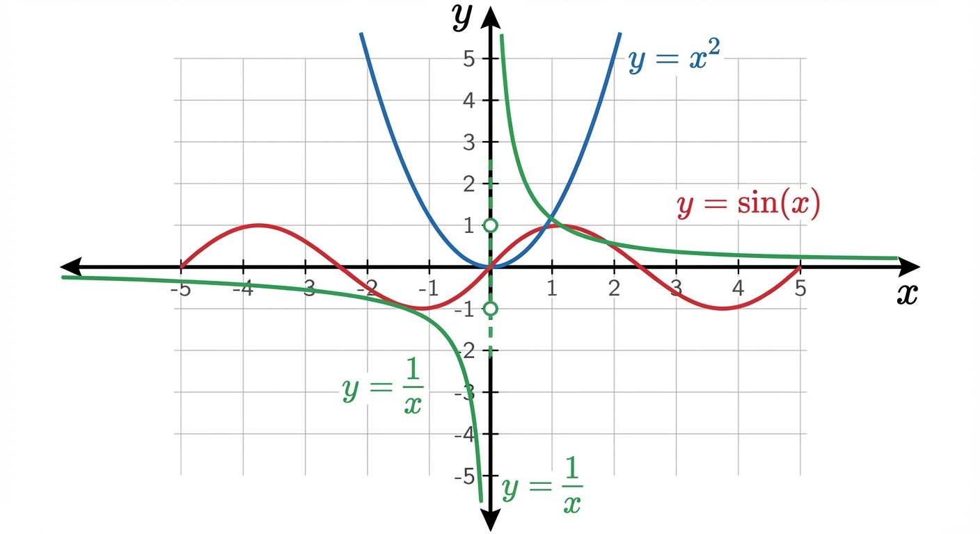
$ python graph_calc.py --functions "x**2,sin(x),1/x" --xmin -10 --xmax 10 --step 0.05
[info] plotting 3 functions
[warn] detected discontinuity candidates near x=0 for 1/x
[output] saved: outputs/graph_bundle.png
[output] legend: y=x^2, y=sin(x), y=1/x

The saved figure clearly shows centered axes, gridlines, and separate branches for 1/x.

The Core Question You Are Answering

“What does a function actually do across a domain, not at just one hand-picked input?”

Concepts You Must Understand First

1. Domain and range
   • Why plotting needs finite windows for infinite mathematical objects.
   • Book Reference: Precalculus (Stewart et al.), function chapters.
2. Sampling theory basics
   • Why step size controls visual fidelity.
   • Book Reference: Doing Math with Python, graph chapter.
3. Discontinuity behavior
   • Why connecting points blindly can create false visuals.
   • Book Reference: introductory calculus continuity sections.

Questions to Guide Your Design

1. How will you represent multiple functions safely (without arbitrary code execution risks)?
2. How will you detect and handle undefined points?
3. How will you make plots comparable across runs?

Thinking Exercise

For y = sin(10x), compare plots using step sizes 1.0, 0.2, and 0.02. Write what information each misses or captures.

The Interview Questions They Will Ask

1. “How does sampling resolution affect accuracy?”
2. “Why are asymptotes hard to plot correctly?”
3. “What makes a plotting pipeline reproducible?”
4. “How would you compare two function families visually?”

Hints in Layers

Hint 1: Starting Point Start with one polynomial and fixed domain.

Hint 2: Next Level Add function registry with predefined safe expressions.

Hint 3: Technical Details Mark NaN/inf values as breaks so lines are not connected across discontinuities.

Hint 4: Tools/Debugging Save both image and CSV of sampled points for inspection.

Books That Will Help

Topic	Book	Chapter
Graphing functions	Doing Math with Python	Ch. 2
Function behavior	Precalculus	Function and graph chapters
Plotting mechanics	Matplotlib docs	Plot and axis guides

Common Pitfalls and Debugging

Problem 1: “Graph looks jagged or wrong”

• Why: step size too coarse.
• Fix: reduce step and re-render.
• Quick test: compare outputs at two step sizes.

Problem 2: “Vertical line jumps across asymptote”

• Why: undefined points not segmented.
• Fix: break line at invalid samples.
• Quick test: plot 1/x and verify separated branches.

Definition of Done

• Tool plots at least three function types (polynomial, trig, rational).
• Discontinuities are handled without fake line bridges.
• Domain, step, and labels are configurable.
• Output is reproducible and saved with metadata.

Project 3: The Ballistics Computer (Trigonometry Simulator)

• File: P03-ballistics-simulator.md
• Main Programming Language: Python
• Alternative Programming Languages: C++, JavaScript, Lua
• Coolness Level: Level 3
• Business Potential: 1
• Difficulty: Level 2
• Knowledge Area: Trigonometry, kinematics, numerical integration
• Software or Tool: Python math library, optional Pygame
• Main Book: Program Arcade Games (Paul Craven)

What you will build: A simulator that converts launch angle and speed into x/y trajectory updates, with optional drag and wind toggles.

Why it teaches this topic: It operationalizes sine/cosine decomposition and accumulation over time.

Core challenges you will face:

• Degrees-to-radians correctness -> Concept: Geometric Modeling
• Stable time stepping (dt) -> Concept: Change, Uncertainty, and Data
• Model assumptions (drag/no drag) -> Concept: Change, Uncertainty, and Data

Real World Outcome

You can run scenarios and compare trajectories under controlled assumptions.

$ python ballistics.py --angle 45 --speed 100 --dt 0.1 --gravity 9.81
[init] vx=70.7107 m/s, vy=70.7107 m/s
[t=0.0] x=0.00 y=0.00
[t=2.0] x=141.42 y=121.80
[t=4.0] x=282.84 y=204.36
...
[event] impact detected at t=14.4
[result] range=1018.23m max_height=254.82m

The Core Question You Are Answering

“How do trig identities become a working physics model over time?”

Concepts You Must Understand First

1. Vector decomposition
   • Why vx = v cos(theta) and vy = v sin(theta).
   • Book Reference: Precalculus trig chapters.
2. Discrete-time updates
   • Why continuous motion can be approximated with small steps.
   • Book Reference: introductory numerical methods notes.
3. Model assumptions
   • What changes when drag is ignored or added.
   • Book Reference: high school mechanics chapters.

Questions to Guide Your Design

1. How small should dt be for stable yet efficient runs?
2. Will you update velocity before or after position each step?
3. How will you detect impact robustly between steps?

Thinking Exercise

Compute by hand the first three updates for vx=10, vy=10, g=1, dt=1. Compare with simulator logs.

The Interview Questions They Will Ask

1. “Why does 45 degrees maximize range in idealized launch?”
2. “What numerical error appears when dt is too large?”
3. “How would you include wind and drag terms?”
4. “What invariants can you use to validate no-drag horizontal motion?”

Hints in Layers

Hint 1: Starting Point Implement no-drag model first with fixed dt.

Hint 2: Next Level Separate state update logic from rendering/printing.

Hint 3: Technical Details Store each step in a trajectory list for later plotting and debugging.

Hint 4: Tools/Debugging Run same input with dt=0.5, 0.1, 0.01 and compare range convergence.

Books That Will Help

Topic	Book	Chapter
Trig and vectors	Precalculus	Trigonometry chapters
Simulation loops	Program Arcade Games	Motion-related chapters
Numerical stepping	Intro numerical methods text	Euler-method intro

Common Pitfalls and Debugging

Problem 1: “Trajectory clearly wrong”

• Why: radians/degrees mismatch.
• Fix: convert angle once at initialization.
• Quick test: compare 30° vs 60° ranges; they should match in no-drag model.

Problem 2: “Projectile tunnels through ground”

• Why: coarse dt misses crossing event.
• Fix: interpolate crossing between final positive and first negative y.
• Quick test: rerun with smaller dt and compare impact location.

Definition of Done

• No-drag simulation returns plausible range and max height.
• Angle unit handling is explicit and tested.
• dt sensitivity documented.
• Output includes deterministic trajectory logs for one golden scenario.

Project 4: The Chaos Game (Fractals & Complex Numbers)

• File: P04-chaos-game.md
• Main Programming Language: Python
• Alternative Programming Languages: Rust, C++, JavaScript
• Coolness Level: Level 5
• Business Potential: 1
• Difficulty: Level 3
• Knowledge Area: Complex numbers, iteration, fractal geometry
• Software or Tool: NumPy, Pillow/Matplotlib
• Main Book: Doing Math with Python

What you will build: A fractal generator (Mandelbrot-style) that maps pixel coordinates to complex plane points and colors by escape-time behavior.

Why it teaches this topic: It turns complex arithmetic and iterative dynamical systems into visual evidence.

Core challenges you will face:

• Complex-plane mapping -> Concept: Geometric Modeling
• Escape-time loop correctness -> Concept: Symbolic and Numeric Algebra
• Performance vs detail tradeoffs -> Concept: Change, Uncertainty, and Data

Real World Outcome

You produce deterministic fractal renders with configurable bounds and iteration limits.

$ python fractal.py --width 1200 --height 800 --max-iter 500 --xmin -2.5 --xmax 1 --ymin -1.2 --ymax 1.2
[info] sampling 960000 pixels
[info] max iterations: 500
[output] wrote outputs/mandelbrot_1200x800.png
[stats] bounded_points=243108 escaped_points=716892

Image output shows recognizable Mandelbrot cardioid and boundary filaments with smooth iteration-based color bands.

The Core Question You Are Answering

“How can a tiny iterative rule create high-complexity structure?”

Concepts You Must Understand First

1. Complex numbers as coordinates
   • Real axis vs imaginary axis interpretation.
   • Book Reference: Doing Math with Python, fractal chapter.
2. Iterative systems
   • Why repeated updates can converge, diverge, or orbit.
   • Book Reference: introductory chaos/fractal notes.
3. Escape criteria
   • Why magnitude threshold indicates divergence.
   • Book Reference: complex dynamics overview resources.

Questions to Guide Your Design

1. How will you map pixel grid to complex-plane bounds?
2. How will you color points based on iteration behavior?
3. What optimizations matter most before parallelization?

Thinking Exercise

Manually iterate z_{n+1} = z_n^2 + c for c=1 and c=-1 starting from z_0=0, then explain why one diverges and one stays bounded.

The Interview Questions They Will Ask

1. “Why is |z| > 2 a valid escape threshold in Mandelbrot checks?”
2. “Where is the algorithm bottleneck and why?”
3. “How would you parallelize pixel evaluation?”
4. “What numeric precision issues can appear at deep zooms?”

Hints in Layers

Hint 1: Starting Point Render low resolution first (e.g., 300x200) to validate mapping.

Hint 2: Next Level Separate coordinate mapping from iteration logic.

Hint 3: Technical Details Use squared magnitude comparison to avoid repeated square roots.

Hint 4: Tools/Debugging Log sample pixel-to-complex mappings at corners and center.

Books That Will Help

Topic	Book	Chapter
Complex numbers in Python	Doing Math with Python	Fractal/geometry chapter
Numerical iteration mindset	Think Complexity (Downey)	Iteration and complexity sections
Visualization workflows	Matplotlib/Pillow docs	Image output basics

Common Pitfalls and Debugging

Problem 1: “Image looks mirrored or shifted”

• Why: incorrect y-axis mapping between image and Cartesian coordinates.
• Fix: document and apply a single coordinate convention.
• Quick test: verify known center point maps to expected complex coordinate.

Problem 2: “Everything appears black or white”

• Why: color mapping not scaled to iteration range.
• Fix: normalize iteration counts before palette mapping.
• Quick test: print min/max iteration values for sampled pixels.

Definition of Done

• Fractal render is reproducible for fixed bounds and iterations.
• Pixel-to-complex mapping is documented and tested.
• Escape-time coloring shows meaningful structure.
• Performance baseline recorded (resolution, runtime, machine).

Project 5: The Monte Carlo Casino (Probability Simulator)

• File: P05-monte-carlo-casino.md
• Main Programming Language: Python
• Alternative Programming Languages: R, Julia, JavaScript
• Coolness Level: Level 3
• Business Potential: 3
• Difficulty: Level 1
• Knowledge Area: Probability, simulation, convergence
• Software or Tool: Python random module, NumPy optional
• Main Book: Think Stats (Allen Downey)

What you will build: A simulator that runs large numbers of trials for dice/card/coin games and compares empirical frequencies to theoretical probabilities.

Why it teaches this topic: It demonstrates variance, convergence, and the law of large numbers with observable data.

Core challenges you will face:

• Correct random-process modeling -> Concept: Change, Uncertainty, and Data
• Efficient counting over many trials -> Concept: Symbolic and Numeric Algebra
• Interpreting variance correctly -> Concept: Change, Uncertainty, and Data

Real World Outcome

You can run deterministic experiments (fixed seed) and compare convergence curves across sample sizes.

$ python monte_carlo.py --game dice7 --trials 100000 --seed 42
[setup] game=dice7, theoretical_p=0.1666667
[run] trials=100000 seed=42
[result] wins=16703 estimate=0.16703
[error] absolute_error=0.00036
[output] convergence table saved: outputs/dice7_convergence.csv

The Core Question You Are Answering

“When does random behavior become statistically predictable?”

Concepts You Must Understand First

1. Independent events
   • Why previous outcomes do not alter fair random next outcomes.
   • Book Reference: Think Stats, probability foundations.
2. Expected value and variance
   • Why two runs can differ while both are valid.
   • Book Reference: introductory probability texts.
3. Convergence diagnostics
   • Why trial count impacts reliability.
   • Book Reference: simulation method chapters.

Questions to Guide Your Design

1. Which games will have known theoretical probabilities for validation?
2. How will you store progress metrics without blowing memory?
3. How will you communicate uncertainty, not only one final number?

Thinking Exercise

Predict outcomes for 10, 100, 1,000, and 100,000 trials of a fair coin before running code. Compare intuition versus observed variance.

The Interview Questions They Will Ask

1. “What is the difference between pseudo-random and truly random?”
2. “Why do we fix seeds during testing?”
3. “How would you estimate confidence intervals for your simulation?”
4. “How do you validate simulator correctness?”

Hints in Layers

Hint 1: Starting Point Implement one simple game with known analytic probability.

Hint 2: Next Level Track cumulative estimate every fixed interval (e.g., every 1,000 trials).

Hint 3: Technical Details Use counters rather than storing every trial result.

Hint 4: Tools/Debugging Run with two different seeds and compare long-run convergence behavior.

Books That Will Help

Topic	Book	Chapter
Probability and simulation	Think Stats	Ch. 1-4
Random APIs	Python docs	random and reproducibility notes
Experimental design basics	Introduction to Probability	early chapters

Common Pitfalls and Debugging

Problem 1: “Simulation never approaches theoretical value”

• Why: biased random generation or wrong event condition.
• Fix: test small deterministic cases and inspect event logic.
• Quick test: run million-trial fair coin; estimate should be near 0.5.

Problem 2: “Different results each run break tests”

• Why: no seed control.
• Fix: expose and log seed.
• Quick test: same seed should reproduce same summary exactly.

Definition of Done

• Simulator supports at least two games with known probabilities.
• Seeded runs are reproducible.
• Convergence metrics are logged and visualizable.
• Error against theoretical baseline is reported.

Project 6: The Secret Message Encoder (Matrix Algebra)

• File: P06-matrix-encoder.md
• Main Programming Language: Python
• Alternative Programming Languages: Julia, MATLAB, Rust
• Coolness Level: Level 3
• Business Potential: 4
• Difficulty: Level 3
• Knowledge Area: Linear algebra, modular arithmetic, classical crypto
• Software or Tool: NumPy
• Main Book: Linear Algebra and Its Applications (Lay et al.)

What you will build: A Hill-cipher style encoder/decoder using matrix multiplication modulo alphabet size.

Why it teaches this topic: It operationalizes matrix transforms and invertibility constraints in a concrete communication workflow.

Core challenges you will face:

• Text/vector representation -> Concept: Symbolic and Numeric Algebra
• Matrix invertibility under modulo arithmetic -> Concept: Geometric Modeling
• Block sizing and padding rules -> Concept: Change, Uncertainty, and Data

Real World Outcome

Your tool can encode and decode short messages deterministically with a valid key matrix.

$ python matrix_cipher.py --mode encode --key "[[3,3],[2,5]]" --text "HELP"
[map] HELP -> [7,4,11,15]
[block] size=2 blocks=2
[result] encoded=DPLE

$ python matrix_cipher.py --mode decode --key "[[3,3],[2,5]]" --text "DPLE"
[result] decoded=HELP
[verify] roundtrip=pass

The Core Question You Are Answering

“How does a matrix transformation scramble information, and what makes reversal possible?”

Concepts You Must Understand First

1. Matrix multiplication rules
   • Shape compatibility and dot-product mechanics.
   • Book Reference: Linear Algebra and Its Applications, early chapters.
2. Invertibility
   • Why singular matrices cannot be reversed.
   • Book Reference: determinant/inverse chapters.
3. Modular arithmetic
   • Why arithmetic wraps around alphabet size.
   • Book Reference: elementary number theory references.

Questions to Guide Your Design

1. How will you enforce valid key matrices for modulo space?
2. What alphabet policy will you support (A-Z only or extended)?
3. How will padding be encoded and stripped safely?

Thinking Exercise

Use a 2x2 key and encode two-letter block by hand under mod 26. Then decode manually and verify exact recovery.

The Interview Questions They Will Ask

1. “Why does determinant coprime condition matter in Hill cipher?”
2. “What is the computational bottleneck in block-matrix encoding?”
3. “Why are classical ciphers insecure against modern attacks?”
4. “How would you design tests for round-trip correctness?”

Hints in Layers

Hint 1: Starting Point Support uppercase A-Z first to simplify mapping.

Hint 2: Next Level Validate key before any encode/decode operation.

Hint 3: Technical Details Separate mapping layer from matrix operation layer for clean tests.

Hint 4: Tools/Debugging Print intermediate numeric blocks for one deterministic sample.

Books That Will Help

Topic	Book	Chapter
Matrix fundamentals	Linear Algebra and Its Applications	Ch. 1-2
Applied Python matrix workflows	NumPy docs	linear algebra routines
Classical crypto perspective	Cracking Codes with Python	relevant cipher chapters

Common Pitfalls and Debugging

Problem 1: “Decode fails even with same key”

• Why: key not invertible modulo 26.
• Fix: enforce determinant coprime check.
• Quick test: run key-validation suite before encoding.

Problem 2: “Garbage characters in output”

• Why: inconsistent text mapping/padding policy.
• Fix: define one strict alphabet contract and padding rule.
• Quick test: round-trip known strings with odd/even lengths.

Definition of Done

• Encode/decode round-trips pass for reference cases.
• Invalid keys are rejected with clear diagnostics.
• Padding behavior is deterministic and documented.
• Numeric intermediate logs available for one debug mode.

Project 7: The Derivative Explorer (Calculus Visualization)

• File: P07-derivative-explorer.md
• Main Programming Language: Python
• Alternative Programming Languages: Julia, JavaScript
• Coolness Level: Level 3
• Business Potential: 2
• Difficulty: Level 2
• Knowledge Area: Differential calculus, numerical approximation
• Software or Tool: Matplotlib, NumPy
• Main Book: Calculus (James Stewart)

What you will build: A tool that estimates derivatives numerically and visualizes both original and derivative curves.

Why it teaches this topic: It exposes derivative as computable local slope and highlights approximation error.

Core challenges you will face:

• Stable finite-difference selection -> Concept: Change, Uncertainty, and Data
• Edge-point handling -> Concept: Symbolic and Numeric Algebra
• Interpretation of noisy estimates -> Concept: Change, Uncertainty, and Data

Real World Outcome

You can run derivative estimation across different step sizes and compare stability.

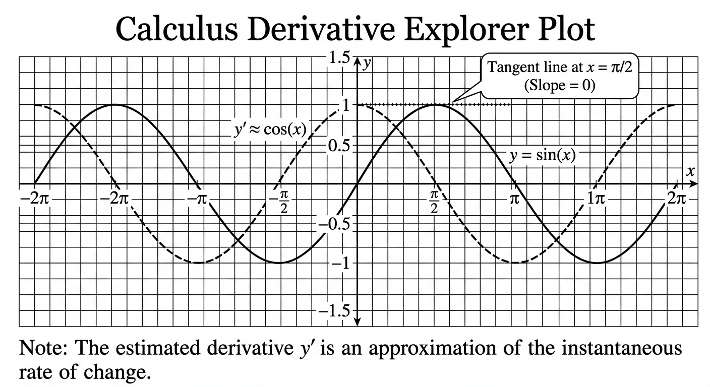
$ python derivative_explorer.py --function "sin(x)" --xmin -6.28 --xmax 6.28 --h 0.001
[info] method=central_difference h=0.001
[metric] max_abs_error_vs_known=0.0012
[output] saved plot: outputs/sin_derivative_compare.png
[output] saved table: outputs/sin_derivative_samples.csv

Plot overlays show original sin(x) and estimated derivative close to cos(x).

The Core Question You Are Answering

“How can a computer estimate instantaneous change from finite samples?”

Concepts You Must Understand First

1. Difference quotient
   • Meaning of f(x+h)-f(x) over h.
   • Book Reference: Calculus, derivative definition chapter.
2. Numerical stability
   • Why smaller h is not always better.
   • Book Reference: numerical methods intro references.
3. Error metrics
   • How to compare estimated and known derivatives.
   • Book Reference: basic error-analysis notes.

Questions to Guide Your Design

1. Will you support forward, backward, and central differences?
2. How will you handle first/last sample points?
3. What diagnostics make method quality visible?

Thinking Exercise

Estimate derivative of x^2 at x=3 with h=1, 0.1, 0.01. Record convergence trend toward true value 6.

The Interview Questions They Will Ask

1. “Why is central difference often preferred?”
2. “What causes catastrophic cancellation in derivative estimates?”
3. “How would you differentiate noisy measured data?”
4. “How do you validate derivative code beyond visual checks?”

Hints in Layers

Hint 1: Starting Point Use one known function with analytic derivative for validation.

Hint 2: Next Level Implement method switch (forward, central) via CLI option.

Hint 3: Technical Details Compute and report max and mean absolute errors.

Hint 4: Tools/Debugging Plot error vs h on logarithmic axis.

Books That Will Help

Topic	Book	Chapter
Derivative foundations	Calculus (Stewart)	Early derivative chapters
Computational math in Python	Doing Math with Python	Calculus chapter
Numeric approximation	Numerical methods primer	finite difference sections

Common Pitfalls and Debugging

Problem 1: “Derivative curve is noisy”

• Why: step size too small with float noise or input spacing issues.
• Fix: sweep h values and pick stable region.
• Quick test: error-vs-h table should show U-shaped behavior.

Problem 2: “Wrong derivative near boundaries”

• Why: using central difference without neighbors.
• Fix: use one-sided formulas at boundaries.
• Quick test: compare edge-point errors separately from interior.

Definition of Done

• Supports at least two finite-difference methods.
• Outputs derivative plot and error metrics.
• Boundary handling is explicit.
• Includes one validated known-function benchmark.

Project 8: The Area Estimator (Integral Calculus)

• File: P08-area-estimator.md
• Main Programming Language: Python
• Alternative Programming Languages: Julia, C++, MATLAB
• Coolness Level: Level 2
• Business Potential: 2
• Difficulty: Level 2
• Knowledge Area: Integral approximation, accumulation
• Software or Tool: Python + Matplotlib
• Main Book: Calculus (James Stewart)

What you will build: A numeric integration tool supporting left, right, midpoint, and trapezoid rules with error comparisons.

Why it teaches this topic: It reveals integration as controlled accumulation and estimator design.

Core challenges you will face:

• Partition strategy -> Concept: Change, Uncertainty, and Data
• Method bias comparison -> Concept: Change, Uncertainty, and Data
• Visualization of approximation geometry -> Concept: Geometric Modeling

Real World Outcome

You can compute area estimates and show improvement as partition count increases.

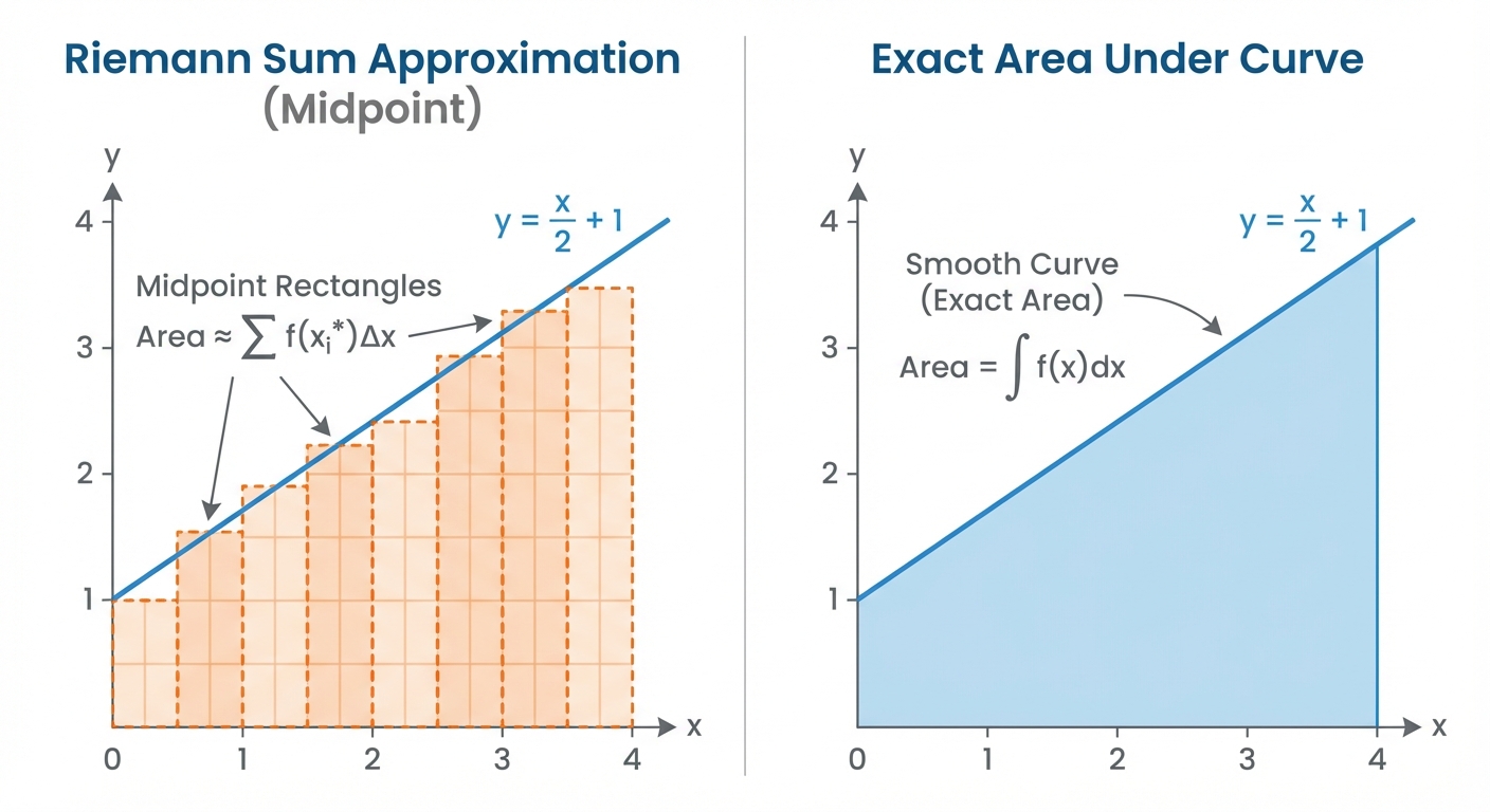
$ python area_estimator.py --function "2*x" --a 0 --b 4 --n 100 --method midpoint
[info] method=midpoint n=100 dx=0.04
[result] estimate=16.0000
[benchmark] analytic=16.0000 abs_error=0.0000
[output] bars plot saved: outputs/riemann_midpoint_100.png

The Core Question You Are Answering

“How do we turn continuous accumulation into a finite, computable process?”

Concepts You Must Understand First

1. Riemann-sum idea
   • Area as sum of many tiny slices.
   • Book Reference: Calculus, integral definition chapter.
2. Method families
   • Why midpoint/trapezoid often outperform one-sided methods.
   • Book Reference: numerical integration notes.
3. Error behavior
   • How error changes with increasing n.
   • Book Reference: basic numerical analysis texts.

Questions to Guide Your Design

1. Which methods and diagnostics will you support initially?
2. How will you compare against known analytic integrals?
3. How will you represent negative area regions?

Thinking Exercise

Estimate integral of f(x)=x on [0,2] with n=2 and n=4 using left and midpoint rules, then compare against true value.

The Interview Questions They Will Ask

1. “Why can midpoint be exact for linear functions?”
2. “How does error scale with partition count?”
3. “What if integrand is discontinuous?”
4. “How would you integrate sampled data points instead of closed-form functions?”

Hints in Layers

Hint 1: Starting Point Implement one method first (left rule), then generalize.

Hint 2: Next Level Abstract sampling point generator per method.

Hint 3: Technical Details Log n, dx, estimate, and error in a table format.

Hint 4: Tools/Debugging Compare method outputs at same n to validate expected ranking.

Books That Will Help

Topic	Book	Chapter
Integral meaning	Calculus (Stewart)	Intro integral chapters
Python numerical workflows	Doing Math with Python	Calculus chapter
Numerical integration	Intro numerical analysis text	quadrature sections

Common Pitfalls and Debugging

Problem 1: “Error does not decrease with larger n”

• Why: bug in partition indexing or method sampling point.
• Fix: test with simple linear function and hand-computed baseline.
• Quick test: midpoint on 2x over [0,4] should be exact.

Problem 2: “Negative areas reported incorrectly”

• Why: misunderstanding signed area.
• Fix: distinguish signed integral and absolute accumulated area.
• Quick test: run symmetric function over symmetric interval.

Definition of Done

• Supports at least three integration methods.
• Reports error against known integral where available.
• Shows error trend as n increases.
• Produces one visualization of geometric approximation.

Project 9: The Data Detective (Linear Regression from Scratch)

• File: P09-linear-regression.md
• Main Programming Language: Python
• Alternative Programming Languages: R, Julia, JavaScript
• Coolness Level: Level 2
• Business Potential: 5
• Difficulty: Level 3
• Knowledge Area: Statistics, optimization, predictive modeling
• Software or Tool: Python, NumPy, Matplotlib
• Main Book: Think Stats

What you will build: A from-scratch linear regression pipeline that loads data, fits y=mx+b, reports metrics, and visualizes residuals.

Why it teaches this topic: It connects algebra, statistics, and numerical evaluation in one practical model.

Core challenges you will face:

• Reliable data preprocessing -> Concept: Symbolic and Numeric Algebra
• Parameter estimation and diagnostics -> Concept: Change, Uncertainty, and Data
• Over-interpretation prevention -> Concept: Change, Uncertainty, and Data

Real World Outcome

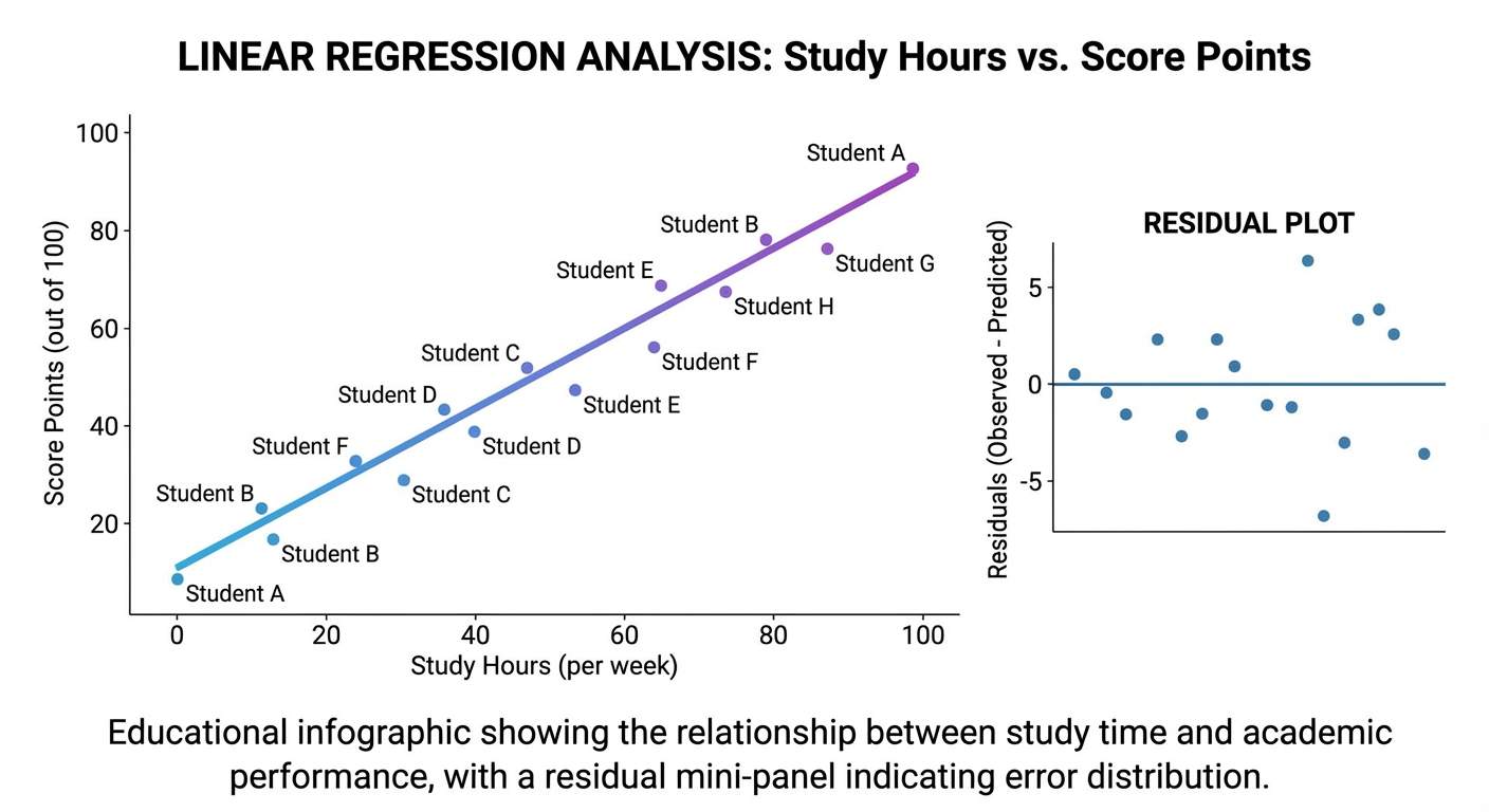
Your tool reads a dataset and produces model parameters, predictions, and diagnostics.

$ python regression.py --csv data/study_hours_vs_score.csv
[load] rows=120 features=1 target=score
[fit] slope=5.18 intercept=30.42
[metric] r2=0.84 mae=4.12
[predict] x=5 -> y=56.32
[output] saved plots: outputs/regression_line.png, outputs/residuals.png

The Core Question You Are Answering

“How do I quantify and validate a relationship in noisy real data?”

Concepts You Must Understand First

1. Mean, variance, covariance
   • Why these summaries underpin linear fit formulas.
   • Book Reference: Think Stats, descriptive statistics chapters.
2. Least-squares objective
   • Why squared residuals are minimized.
   • Book Reference: intro regression texts.
3. Model diagnostics
   • Why one metric is insufficient.
   • Book Reference: residual analysis resources.

Questions to Guide Your Design

1. How will you handle missing or malformed rows?
2. Which fit method will you implement first (closed-form vs iterative)?
3. What diagnostics are mandatory before claiming model quality?

Thinking Exercise

Given three points, compute slope/intercept by hand and compare with your implementation’s output.

The Interview Questions They Will Ask

1. “Why do we square residuals instead of absolute value by default?”
2. “What does R-squared not tell you?”
3. “How do outliers affect linear regression?”
4. “When would gradient descent be preferable to closed-form?”

Hints in Layers

Hint 1: Starting Point Implement closed-form slope/intercept for single-feature regression first.

Hint 2: Next Level Add residual plot generation to catch hidden pattern errors.

Hint 3: Technical Details Create a deterministic train/test split strategy with fixed seed.

Hint 4: Tools/Debugging Use synthetic linear data with known slope/intercept for sanity checks.

Books That Will Help

Topic	Book	Chapter
Statistical foundations	Think Stats	Ch. 2-8
Regression intuition	An Introduction to Statistical Learning	linear regression chapter
Numeric implementation	NumPy docs	array ops for vectorized stats

Common Pitfalls and Debugging

Problem 1: “Excellent metric but poor predictions on new points”

• Why: overfitting or domain extrapolation.
• Fix: evaluate on held-out data and avoid unsupported ranges.
• Quick test: compare train vs test metrics.

Problem 2: “Fit unstable with slight data change”

• Why: outlier sensitivity.
• Fix: inspect residuals and test robust alternatives.
• Quick test: remove top outlier and compare parameter shift.

Definition of Done

• Closed-form linear regression implemented from scratch.
• Metrics include at least R2 and MAE.
• Residual plot generated and interpreted.
• Data-cleaning and split policy documented.

Project 10: The 3D Renderer (Linear Algebra & Projection)

• File: P10-3d-renderer.md
• Main Programming Language: Python
• Alternative Programming Languages: C++, Rust, JavaScript
• Coolness Level: Level 5
• Business Potential: 1
• Difficulty: Level 4
• Knowledge Area: 3D geometry, matrices, projection
• Software or Tool: Pygame/Matplotlib + NumPy
• Main Book: Computer Graphics from Scratch (Gabriel Gambetta)

What you will build: A wireframe renderer that projects 3D cube vertices onto 2D screen space and supports interactive rotation.

Why it teaches this topic: It converts linear algebra and trigonometry into a direct visual system.

Core challenges you will face:

• 3D-to-2D projection math -> Concept: Geometric Modeling
• Transform order correctness -> Concept: Geometric Modeling
• Numerical stability across frames -> Concept: Change, Uncertainty, and Data

Real World Outcome

You launch a window displaying a rotating cube whose depth perception changes with camera distance and field-of-view settings.

$ python renderer3d.py --fov 90 --camera-z 5 --rotation-speed 0.02
[init] vertices=8 edges=12
[frame 001] avg_depth=5.12 projected_points=8
[frame 240] rotation_y=4.80 rad
[event] key LEFT -> rotation_y -= 0.1
[event] key RIGHT -> rotation_y += 0.1

Observed behavior: front edges appear larger than back edges; incorrect camera parameters trigger obvious distortion warnings.

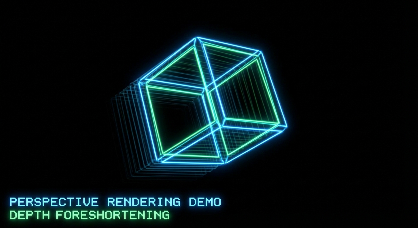
The Core Question You Are Answering

“How does linear algebra create the illusion of depth on a flat display?”

Concepts You Must Understand First

1. Coordinate frames
   • Object space, world space, view space, screen space.
   • Book Reference: Computer Graphics from Scratch, early chapters.
2. Rotation and projection matrices
   • Why matrix order affects visual output.
   • Book Reference: linear algebra transformation chapters.
3. Perspective divide
   • Why depth scales apparent size.
   • Book Reference: graphics projection materials.

Questions to Guide Your Design

1. How will you store vertices, edges, and transforms cleanly?
2. How will you prevent division by near-zero depth?
3. Which invariants verify rotation correctness?

Thinking Exercise

Project two points at equal x/y but different z values. Explain why farther point appears closer to center.

The Interview Questions They Will Ask

1. “Why are transformation pipelines usually matrix-based?”
2. “What goes wrong when transform order is reversed?”
3. “What is gimbal lock and how can it be mitigated?”
4. “How would you optimize rendering beyond wireframe?”

Hints in Layers

Hint 1: Starting Point Render static cube before adding animation.

Hint 2: Next Level Implement one-axis rotation, validate invariants, then add more axes.

Hint 3: Technical Details Normalize camera and projection parameters in one config object.

Hint 4: Tools/Debugging Log projected coordinates for one vertex across frames to detect drift.

Books That Will Help

Topic	Book	Chapter
Graphics pipeline	Computer Graphics from Scratch	Ch. 1-3
Matrix transforms	Linear Algebra and Its Applications	transform sections
Python rendering setup	Pygame docs	display and draw primitives

Common Pitfalls and Debugging

Problem 1: “Cube explodes or flips unpredictably”

• Why: transform order or coordinate-frame mix-up.
• Fix: enforce explicit pipeline order and test each stage independently.
• Quick test: rotate 90 degrees around one axis and compare expected coordinates.

Problem 2: “Massive distortion near camera”

• Why: depth close to zero in perspective divide.
• Fix: clamp near plane and reject invalid depth values.
• Quick test: move camera z and verify stable projection bounds.

Definition of Done

• Wireframe cube renders with perspective.
• Rotation controls work predictably.
• Transform order is documented and tested.
• Near-plane and invalid-depth safeguards implemented.

Project 11: The Epidemic Simulator (Exponential Growth)

• File: P11-epidemic-simulator.md
• Main Programming Language: Python
• Alternative Programming Languages: NetLogo, Julia, JavaScript
• Coolness Level: Level 2
• Business Potential: 3
• Difficulty: Level 3
• Knowledge Area: Exponential growth, compartment models, simulation
• Software or Tool: Python, Matplotlib/Pygame
• Main Book: Doing Math with Python

What you will build: A discrete-time epidemic simulator (SIR-style) with configurable transmission and recovery parameters, plus trend charts.

Why it teaches this topic: It makes exponential growth, saturation, and intervention effects visible and testable.

Core challenges you will face:

• State-transition correctness -> Concept: Change, Uncertainty, and Data
• Parameter sensitivity analysis -> Concept: Change, Uncertainty, and Data
• Visualization of multi-series dynamics -> Concept: Geometric Modeling

Real World Outcome

You can run scenarios and compare infection-curve shapes under different policies.

$ python epidemic.py --population 1000 --infected 5 --beta 0.30 --gamma 0.10 --days 120 --seed 7
[init] S=995 I=5 R=0
[day 20] S=702 I=242 R=56
[day 45] S=310 I=401 R=289
[day 80] S=188 I=95 R=717
[result] peak_infected=418 on day 42
[output] saved: outputs/sir_curves_seed7.png

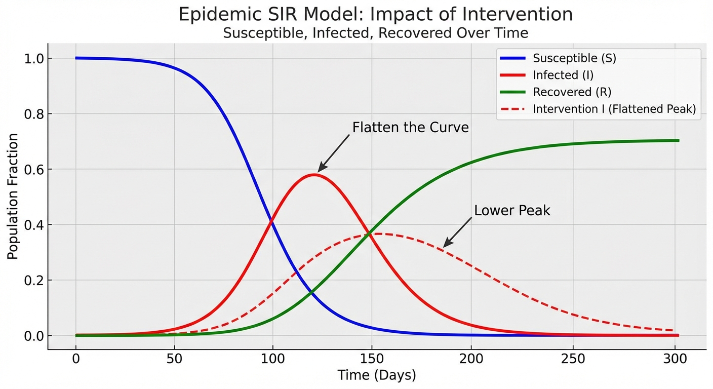
The Core Question You Are Answering

“Why can small parameter changes create dramatically different system outcomes?”

Concepts You Must Understand First

1. Exponential growth intuition
   • Why early growth looks slow and then accelerates.
   • Book Reference: exponential functions in pre-calculus text.
2. Compartment-model transitions
   • How S -> I -> R updates work per time step.
   • Book Reference: intro epidemiological modeling notes.
3. Scenario analysis
   • Why one run is not enough for interpretation.
   • Book Reference: simulation methodology resources.

Questions to Guide Your Design

1. How will you represent people/states efficiently?
2. How will you enforce deterministic runs for debugging?
3. How will you compare interventions (e.g., lowering beta) fairly?

Thinking Exercise

With fixed recovery rate, vary transmission rate across three values and predict peak timing/order before running simulation.

The Interview Questions They Will Ask

1. “What does the basic reproduction concept represent intuitively?”
2. “How do deterministic and stochastic epidemic models differ?”
3. “How would you calibrate such a model against real data?”
4. “What are major limitations of simple SIR assumptions?”

Hints in Layers

Hint 1: Starting Point Implement deterministic compartment counts before agent-level simulation.

Hint 2: Next Level Add seed-controlled stochastic transitions.

Hint 3: Technical Details Separate transition logic from plotting/output.

Hint 4: Tools/Debugging Log compartment totals each step and assert they always sum to population.

Books That Will Help

Topic	Book	Chapter
Exponential and logistic behavior	Precalculus text	growth-model sections
Python modeling practice	Doing Math with Python	calculus/modeling chapter
Intro epidemiological modeling	public-health modeling notes	SIR intro

Common Pitfalls and Debugging

Problem 1: “Population totals drift over time”

• Why: inconsistent state updates or double-counting transitions.
• Fix: use staged updates per time step.
• Quick test: assert S+I+R == N every day.

Problem 2: “Conclusions change wildly run to run”

• Why: stochastic model without seed control or replication.
• Fix: run multi-seed batches and report distribution of outcomes.
• Quick test: compare peak statistics across fixed seed set.

Definition of Done

• Simulator maintains population invariants.
• Seed control and scenario comparisons are supported.
• Outputs include peak timing and magnitude.
• At least two intervention scenarios are compared in one report.

Project Comparison Table

Project	Difficulty	Time	Depth of Understanding	Fun Factor
1. Equation Solver	Level 1	Weekend	High	★★☆☆☆
2. Graphing Calculator	Level 1-2	Weekend	Medium	★★★☆☆
3. Ballistics Simulator	Level 2	2-3 days	High	★★★★☆
4. Chaos Game	Level 3	1 week	Deep	★★★★★
5. Monte Carlo Casino	Level 1	Weekend	Medium	★★★☆☆
6. Matrix Encoder	Level 3	1 week	High	★★★★☆
7. Derivative Explorer	Level 2	2-3 days	High	★★★☆☆
8. Area Estimator	Level 2	2-3 days	High	★★★☆☆
9. Linear Regression	Level 3	1 week	High	★★★★☆
10. 3D Renderer	Level 4	2+ weeks	Deep	★★★★★
11. Epidemic Simulator	Level 3	1 week	High	★★★★☆

Recommendation

If you are new to this topic: Start with Project 1, then Project 2, then Project 5. This sequence builds parsing, graphing, and simulation confidence quickly.

If you are visually motivated: Start with Project 3 and Project 4. You will get immediate geometric feedback that makes formulas intuitive.

If you want data/AI foundations: Prioritize Project 5, Project 8, and Project 9 before anything else.

If you want the hardest path: Tackle Project 6, Project 10, and Project 11 after finishing the primer.

Final Overall Project: The PyMath Engine

The Goal: Combine Projects 1, 2, 7, 8, and 9 into a single modular engine that parses expressions, computes derivatives/integrals numerically, fits basic models, and visualizes results.

1. Build an expression pipeline (parse -> normalize -> evaluate -> verify).
2. Add analytical tools (differentiate, integrate, fit_line) with diagnostic outputs.
3. Add a visualization layer for curves, derivatives, integrals, and residual plots.
4. Add scenario runner for uncertainty experiments (seeded Monte Carlo modules).

Success Criteria: deterministic input/output contracts, validation diagnostics for every module, and one end-to-end demo notebook/report.

From Learning to Production: What Is Next

Your Project	Production Equivalent	Gap to Fill
Equation Solver	CAS tools (SymPy/Mathematica)	richer parser grammar, symbolic simplification breadth
Graphing Calculator	Scientific plotting platforms	performance, interactive UX, large-data handling
Monte Carlo Simulator	Risk engines and experimentation services	parallelization, uncertainty intervals, data pipelines
Regression Tool	ML analytics platforms	feature engineering, regularization, model governance
3D Renderer	Graphics/game engines	full rasterization pipeline, shading, asset systems

Summary

This learning path covers high school mathematics through 11 real projects that force you to model, compute, validate, and explain outcomes.

#	Project Name	Main Language	Difficulty	Time Estimate
1	Homework Destroyer	Python	Level 1	4-8h
2	Visual Graphing Calculator	Python	Level 1-2	4-8h
3	Ballistics Computer	Python	Level 2	8-16h
4	Chaos Game	Python	Level 3	10-20h
5	Monte Carlo Casino	Python	Level 1	4-8h
6	Secret Message Encoder	Python	Level 3	10-20h
7	Derivative Explorer	Python	Level 2	8-16h
8	Area Estimator	Python	Level 2	8-16h
9	Data Detective	Python	Level 3	12-24h
10	3D Renderer	Python	Level 4	20-40h
11	Epidemic Simulator	Python	Level 3	12-24h

Expected Outcomes

• You can implement core high-school math concepts as reproducible computational systems.
• You can diagnose numeric/model errors using residuals, invariants, and convergence checks.
• You can communicate assumptions, limitations, and verification evidence like an engineer.

Additional Resources and References

Standards and Specifications

• Python Language Reference
• NumPy User Guide
• Matplotlib User Guide
• SymPy Documentation

Industry and Education Signals

• U.S. Bureau of Labor Statistics: Math Occupations Outlook
• NAGB 2025 NAEP Release
• OECD PISA 2022 Results
• GitHub Octoverse 2025

Books

• Doing Math with Python by Amit Saha - practical bridge from formulas to implementation.
• Think Stats by Allen B. Downey - data and simulation mindset.
• Linear Algebra and Its Applications by Lay, Lay, and McDonald - matrix intuition for transformations.
• Calculus by James Stewart - derivative/integral foundations used in numerical approximations.
• Computer Graphics from Scratch by Gabriel Gambetta - geometric rendering pipeline from first principles.

Curriculum Alignment Addendum (2026): High School Core Completion

This append-only addendum keeps every original section intact and extends coverage to include the missing high-school-to-college bridge topics identified in the conversation:

• Formal logic and proof techniques
• Inequalities and absolute value reasoning
• Sequences and series (finite/infinite behavior intuition)
• Conic sections
• Deeper vectors and matrices foundations
• Complex numbers in rectangular and polar form
• Function theory (domain, inverse, composition, piecewise behavior)
• Mathematical modeling with units, assumptions, and error analysis
• Combinatorics and counting principles

Important scope note about Monte Carlo The original Monte Carlo project remains valuable as an enrichment project. In typical high-school curricula (U.S. and Brazil), Monte Carlo is usually optional/extension, while probability foundations are core. This addendum fills that core-first ordering without removing any existing advanced material.

Curriculum references used for alignment

• U.S. Common Core State Standards for High School Mathematics (conceptual categories N, A, F, G, S): Common Core Mathematics Standards
• Brazil BNCC (Ensino Medio, Matematica e suas Tecnologias): BNCC official document

High School Curriculum Coverage Matrix (Addendum)

Curriculum Cluster	Typical High School Scope	Where This Guide Covers It (Original + Addendum)	College Bridge Value
Algebra and Equations	Linear/quadratic systems, manipulation, identities	Projects 1, 12, 13, 17	Required for calculus, linear algebra, CS reasoning
Function Analysis	Domain/range, composition, inverse, piecewise, asymptotes	Projects 2, 19	Critical for calculus and modeling
Geometry and Trigonometry	Coordinate geometry, circles, triangles, trig ratios	Projects 3, 15, 16	Required for physics, graphics, engineering
Conic Sections	Parabola, ellipse, hyperbola forms and parameters	Project 15	Foundation for analytic geometry and multivariable math
Sequences and Series	Arithmetic/geometric sequences, sigma notation	Project 14	Direct prep for Calculus II and discrete math
Vectors	Magnitude, direction, dot product, decomposition	Projects 3, 10, 16	Needed for linear algebra and mechanics
Matrices and Systems	Matrix ops, determinants, solving linear systems	Projects 6, 10, 17	Core for linear algebra and data science
Complex Numbers	a+bi, polar form, roots, geometric view	Projects 4, 18	Essential for signals, control, advanced algebra
Counting and Probability	Permutations/combinations, probability models	Projects 5, 20	Basis for statistics, CS algorithms
Statistics and Data	Regression, uncertainty, interpretation	Projects 9, 11, 20	Foundation for data science and inference
Proof and Logic	Implication, quantifiers, induction, contradiction	Project 12	Essential for discrete math and rigorous reasoning
Modeling and Units	Assumptions, dimensional analysis, error propagation	Projects 3, 11, 20	Key for engineering and scientific computing

Theory Primer Addendum: Missing High School Foundations

Concept A: Logic and Proof Methods

Fundamentals Logic is the grammar of mathematical truth. High school often teaches answers, but college math asks for justified claims. You need statements, connectives (and, or, not, implies), and quantifiers (for all, there exists). Proof methods such as direct proof, contradiction, and induction are not optional extras; they are the mechanism that turns intuition into reliable conclusions. In programming terms, proofs are your formal test suite for general statements.

Deep Dive A strong beginner mental model is: definitions -> assumptions -> legal inference steps -> conclusion. If any link is vague, the argument is weak. Direct proof works when the conclusion structure follows naturally from known properties. Contradiction is useful when proving impossibility or uniqueness: assume the opposite, derive inconsistency, reject the assumption. Induction is a two-stage loop invariant on natural numbers: base case initializes truth; induction step preserves truth from n to n+1. Quantifiers are where most errors occur. for all x, exists y is not the same as exists y, for all x; the order changes meaning. In software design, this maps to API guarantees and constraints. Failure modes include hidden assumptions, domain mismatch (integers vs reals), and proving only examples rather than general case.

How this fits on projects Project 12 leads directly; Projects 1, 17, 19 reuse proof discipline for correctness arguments.

Definitions & key terms

• Proposition: statement with truth value.
• Predicate: statement depending on variable.
• Quantifier: scope operator (forall, exists).
• Contradiction: logical impossibility.
• Induction hypothesis: assumed truth for step proof.

Mental model diagram

[Definitions] -> [Assumptions] -> [Inference Rules] -> [Conclusion]
      ^                                                  |
      |----------------- verification loop --------------|
Failure modes: hidden assumptions | quantifier swap | domain mismatch

How it works

1. Define objects and domain precisely.
2. State what must be proved.
3. Pick proof method that matches claim structure.
4. Execute legal inference steps with no jumps.
5. Validate no domain assumptions were smuggled.

Minimal concrete example

Claim: Sum of two odd integers is even.
Let a=2k+1, b=2m+1.
a+b = 2(k+m+1), which is divisible by 2.
Therefore a+b is even.

Common misconceptions

• Checking many examples is not a proof.
• A true conclusion with invalid reasoning is still wrong mathematics.

Check-your-understanding questions

1. Why does quantifier order matter?
2. When is contradiction better than direct proof?
3. What breaks an induction proof?

Check-your-understanding answers

1. It changes who depends on whom (y may depend on x, or not).
2. When direct construction is hard but impossibility is easy to derive.
3. Missing/false base case, invalid induction transition, or wrong domain.

Real-world applications Program verification, algorithm correctness, cryptography arguments.

Where you will apply it Project 12 primary; Projects 17 and 19 secondary.

Key insight Proof is structured debugging of mathematical claims.

Summary Logic and proof methods convert symbolic manipulation into trustworthy reasoning.

Homework/Exercises

1. Prove: product of two consecutive integers is even.
2. Disprove: all prime numbers are odd.
3. Inductively prove: 1+2+...+n = n(n+1)/2.

Solutions

1. Let n and n+1; one is even, so product is even.
2. Counterexample: 2 is prime and even.
3. Base case n=1 holds; induction step adds n+1 to both sides and factors.

Concept B: Inequalities and Absolute Value

Fundamentals Inequalities describe ranges, not single points. Absolute value encodes distance from zero, making it ideal for error bounds and tolerance reasoning. High school fluency requires translating symbolic inequalities into interval notation and number-line geometry.

Deep Dive The main cognitive shift is from equation solving to set solving. For x^2 < 9, the answer is not x=3; it is the interval (-3, 3). Sign analysis becomes crucial when multiplying/dividing inequalities: multiplying by a negative flips inequality direction, a common source of mistakes. Absolute value introduces piecewise structure: |x-a| < r means distance from a is less than r, equivalent to a-r < x < a+r. For |x-a| > r, solutions split into two outer intervals. Graphical interpretation prevents algebra-only errors. In modeling, inequalities represent constraints and feasibility regions. In optimization, they define allowable design spaces. Failure modes include forgetting domain restrictions, mishandling boundary inclusion (< vs <=), and applying equation techniques mechanically to inequality systems. Python visualization helps by plotting regions and validating random points against constraints.

How this fits on projects Project 13 primary; Projects 1, 19, and 20 apply bound reasoning.

Definitions & key terms

• Feasible region: set of values satisfying all constraints.
• Interval notation: compact range representation.
• Closed/open boundary: included/excluded endpoint.
• Compound inequality: two constraints joined by and or or.

Mental model diagram

Symbolic constraint -> Interval(s) -> Number line / region view -> Validation points
      |                    |                    |                         |
      +--------------------+--------------------+-------------------------+
                      invariant: same solution set

How it works

1. Isolate expression when possible.
2. Track sign flips under multiplication/division.
3. Convert absolute value to piecewise linear constraints.
4. Express answers in intervals and graph.
5. Validate with sample points inside/outside boundaries.

Minimal concrete example

|2x-4| <= 6
-6 <= 2x-4 <= 6
-2 <= 2x <= 10
-1 <= x <= 5

Common misconceptions

• Absolute value can never be negative, but expressions inside can.
• |x| < a and |x| > a are not solved the same way.

Check-your-understanding questions

1. Why does multiplying by -1 flip inequality direction?
2. Convert |x+2| > 3 to intervals.
3. How do you represent strict vs inclusive bounds?

Check-your-understanding answers

1. Ordering reverses on the number line under sign inversion.
2. x > 1 or x < -5.
3. Parentheses for strict, brackets for inclusive.

Real-world applications Tolerance windows in manufacturing, risk limits in finance, input validation.

Where you will apply it Project 13 primary; Projects 19 and 20 secondary.

Key insight Inequalities model admissible reality, not exact equality.

Summary Absolute value and inequalities are foundational for error bounds and optimization.

Homework/Exercises

1. Solve 3-2x > 7.
2. Solve |x-1| < 4.
3. Solve system: x >= -2 and x < 5 and |x| > 1.

Solutions

1. x < -2.
2. -3 < x < 5.
3. [-2, -1) U (1, 5).

Concept C: Sequences and Series

Fundamentals Sequences describe ordered values indexed by position; series describe accumulated sums. They connect algebraic patterns to limits and recursive thinking, making them central to pre-calculus and college transition.

Deep Dive Arithmetic and geometric sequences are core. Arithmetic adds constant difference; geometric multiplies by constant ratio. Closed forms (a_n) and recursive forms (a_{n+1} from a_n) offer two reasoning modes: direct lookup and process simulation. Sigma notation compresses repetitive sums and prepares students for integral and algorithmic complexity thinking. Infinite geometric series converge only when |r| < 1, a critical bridge to limit intuition. Recursive sequences model feedback systems and compounding behavior. Failure modes include confusing term value with partial sum, misusing formulas outside assumptions, and treating divergence as failure instead of valid classification.

How this fits on projects Project 14 primary; Projects 11 and 20 reuse growth and accumulation models.

Definitions & key terms

• Sequence, nth term, recursive definition, partial sum, convergence.

Mental model diagram

Index n -> Term a_n -> Partial sums S_n -> Limit behavior (converge/diverge)

How it works

1. Identify pattern type or construct recurrence.
2. Compute/derive explicit term rule.
3. Build partial sums and trend diagnostics.
4. Classify convergence or divergence.
5. Explain implication for model stability.

Minimal concrete example

Geometric sequence: a1=3, r=2
Terms: 3,6,12,24,...
S4 = 3+6+12+24 = 45

Common misconceptions

• A sequence can diverge and still be meaningful.
• Recursive definition is not inferior to explicit formula.

Check-your-understanding questions

1. Difference between a_n and S_n?
2. When does geometric series converge?
3. Why recursion is useful in simulation?

Check-your-understanding answers

1. Term value vs cumulative sum.
2. |r| < 1.
3. Many real systems update from previous state.

Real-world applications Loan growth, depreciation, population models, iterative algorithms.

Where you will apply it Project 14 primary; Project 11 secondary.

Key insight Sequences are state evolution; series are accumulated effect.

Summary Sequences/series build the bridge from algebra to calculus and algorithms.

Homework/Exercises

1. Find explicit formula for arithmetic sequence 5,8,11,....
2. Compute S10 for same sequence.
3. Determine convergence of geometric series with r=1.2.

Solutions

1. a_n = 5 + 3(n-1).
2. S10 = 185.
3. Diverges because |r| > 1.

Concept D: Conic Sections and Coordinate Geometry

Fundamentals Conics are geometric loci defined by distance constraints. Their algebraic forms connect graph shape to parameters, giving students a high-leverage tool for analytic geometry.

Deep Dive Parabolas model equal distance from a focus and directrix, ellipses model constant sum of distances to two foci, and hyperbolas model constant difference. Standard forms make center/orientation visible, while completing the square converts general quadratic equations into interpretable forms. Translating and scaling conics develops geometric transformation thinking. Failure modes include sign mistakes in standard forms, confusion between major/minor axes, and ignoring domain/physical feasibility in applications.

How this fits on projects Project 15 primary; Projects 2 and 3 reuse shape intuition.

Definitions & key terms Focus, directrix, vertex, eccentricity, major axis, asymptotes.

Mental model diagram

General quadratic -> Complete square -> Standard form -> Geometric parameters -> Graph

How it works

1. Group x/y terms and constants.
2. Complete square by variable groups.
3. Normalize to standard conic form.
4. Extract center, radii, focal parameters.
5. Validate by sampled points and symmetry checks.

Minimal concrete example

x^2 + y^2 - 4x + 6y - 12 = 0
(x-2)^2 + (y+3)^2 = 25
Circle center (2,-3), radius 5

Common misconceptions

• Conics are not only memorization tables; they are transformable models.
• Same quadratic degree can represent different shapes depending on signs/coefs.

Check-your-understanding questions

1. What sign pattern distinguishes ellipse vs hyperbola?
2. Why complete the square?
3. How do translations affect conic graphs?

Check-your-understanding answers

1. Ellipse has same sign x^2 and y^2 terms; hyperbola opposite signs.
2. To recover geometric parameters from algebraic form.
3. Shift center, preserve intrinsic shape.

Real-world applications Orbits, optics, radio localization, projectile approximations.

Where you will apply it Project 15 primary.

Key insight Conics unify algebraic manipulation and geometric interpretation.

Summary Conic mastery builds analytic geometry fluency for calculus and physics.

Homework/Exercises

1. Convert x^2 - 6x + y^2 + 8y = 0 to standard form.
2. Classify 9x^2 + 4y^2 = 36.
3. Find asymptotes of x^2 - y^2 = 1.

Solutions

1. (x-3)^2 + (y+4)^2 = 25.
2. Ellipse.
3. y = +/-x.

Concept E: Vectors and Matrices for High School-to-College Bridge

Fundamentals Vectors represent magnitude and direction; matrices represent linear transformations and system organization. Together they form the language of modern quantitative fields.

Deep Dive In 2D/3D, vectors support displacement, velocity decomposition, and directional reasoning. Dot product links geometry and algebra: angle, projection, orthogonality. Matrices compactly encode transformations (rotation, scaling, shear) and equation systems. Determinants indicate invertibility and area/volume scaling behavior. Solving linear systems via elimination or matrix methods introduces structural thinking central to college linear algebra. Failure modes include dimension mismatch, row/column order confusion, and assuming commutativity of multiplication.

How this fits on projects Projects 16 and 17 primary; Projects 3, 6, and 10 secondary.

Definitions & key terms Vector norm, unit vector, dot product, matrix inverse, determinant, rank.

Mental model diagram

Geometry question <-> Vector representation <-> Matrix operation <-> Interpretation

How it works

1. Represent quantities as vectors/matrices with explicit dimensions.
2. Apply legal operations respecting shape constraints.
3. Interpret numeric output geometrically (angle, scale, orientation).
4. Validate via invariant checks (orthogonality, reconstruction error).

Minimal concrete example

v=(3,4) => ||v||=5
u=(1,0)
v dot u = 3 => projection of v on x-axis is 3

Common misconceptions

• Matrix multiplication order matters.
• Dot product is scalar, not vector.

Check-your-understanding questions

1. Why can AB exist while BA may not?
2. What does zero dot product indicate?
3. Why determinant zero matters?

Check-your-understanding answers

1. Dimensions may align only one way.
2. Orthogonality (for nonzero vectors).
3. Matrix is non-invertible; system may lack unique solution.

Real-world applications Graphics, robotics, optimization, statistics.

Where you will apply it Projects 16, 17 primary; 6 and 10 secondary.

Key insight Vectors/matrices are not optional add-ons; they are the computational geometry backbone.

Summary This concept cluster is the most direct bridge to college engineering math.

Homework/Exercises

1. Compute angle between (1,1) and (1,-1).
2. Solve a 2x2 system by elimination.
3. Test invertibility of [[1,2],[2,4]].

Solutions

1. 90 degrees.
2. Depends on system chosen; verify by substitution.
3. Determinant zero, not invertible.

Concept F: Complex Numbers and Polar Form

Fundamentals Complex numbers extend real numbers to solve equations like x^2 + 1 = 0. They are points/vectors in a plane, not mysterious symbols.

Deep Dive Rectangular form a+bi and polar form r(cos theta + i sin theta) provide complementary views. Rectangular is convenient for addition/subtraction; polar excels for multiplication, division, and powers. Euler’s identity links exponential and trigonometric behavior, giving a compact representation for oscillatory systems. Conjugates simplify division and magnitude computation. Failure modes include sign errors with i^2=-1, incorrect angle quadrant, and mixing degrees/radians.

How this fits on projects Project 18 primary; Project 4 secondary.

Definitions & key terms Real part, imaginary part, modulus, argument, conjugate, roots of unity.

Mental model diagram

a+bi <-> point (a,b) <-> polar (r,theta) <-> geometric operations

How it works

1. Convert between rectangular and polar forms.
2. Apply operation in the best representation.
3. Convert back if interpretation needs components.
4. Validate via modulus/argument consistency.

Minimal concrete example

z=1+i
|z|=sqrt(2), arg=45 degrees
z^2=(1+i)^2=2i

Common misconceptions

• Imaginary does not mean unreal.
• Polar form is not only for advanced math; it simplifies operations.

Check-your-understanding questions

1. Why use conjugate when dividing complex numbers?
2. What is geometric meaning of multiplying by i?
3. How do roots of unity distribute on plane?

Check-your-understanding answers

1. To remove imaginary part from denominator.
2. Rotation by 90 degrees.
3. Equally spaced points on unit circle.

Real-world applications Signal processing, AC circuits, control systems, fractals.

Where you will apply it Project 18 primary; Project 4 secondary.

Key insight Complex numbers are geometry plus algebra in one object.

Summary Polar/rectangular fluency prepares students for physics and engineering math.

Homework/Exercises

1. Convert -1 + sqrt(3)i to polar.
2. Compute (2cis30)/(cis10) in polar shorthand.
3. Find cube roots of unity.

Solutions

1. r=2, angle 120 degrees.
2. 2cis20.
3. 1, cis120, cis240.

Concept G: Function Theory and Modeling Discipline

Fundamentals Function mastery means understanding structure: domain, codomain behavior, composition, inversion conditions, piecewise definitions, asymptotic trends, and model validity.

Deep Dive Many students can compute f(3) but cannot explain where f is undefined or whether an inverse exists. College math demands that structural rigor. Domain restrictions prevent illegal operations (division by zero, invalid roots/log arguments). Composition models multi-stage systems, and inverse functions encode reversibility. Piecewise functions model rule changes across regimes, common in pricing, physics thresholds, and policy models. Modeling discipline adds units, assumptions, parameter sensitivity, and error propagation. A model is only as good as its assumptions and validation evidence. Failure modes include unit inconsistency, overfitting, extrapolation abuse, and hiding uncertainty.

How this fits on projects Projects 19 and 20 primary; Projects 2, 3, 9, and 11 secondary.

Definitions & key terms Domain, codomain, invertibility, piecewise continuity, dimensional consistency, sensitivity.

Mental model diagram

Real-world question -> assumptions -> function model -> parameter fit -> validation -> decision

How it works

1. Define measurable quantities and units.
2. Propose functional relationship and constraints.
3. Fit/estimate parameters from data.
4. Validate on holdout or sanity scenarios.
5. Communicate uncertainty and boundaries.

Minimal concrete example

Taxi fare model:
fare(d) = 4.50 + 1.20*d, for d>=0
Check units: dollars + dollars/km * km -> dollars

Common misconceptions

• Good fit on one dataset does not guarantee predictive validity.
• Inverse exists only under appropriate monotonic/injective behavior.

Check-your-understanding questions

1. Why must domain be explicit before plotting?
2. What does dimensional inconsistency reveal?
3. Why is extrapolation risky?

Check-your-understanding answers

1. Undefined regions can invalidate interpretation.
2. Model equation is physically/mathematically invalid.
3. Relationship may break outside observed range.

Real-world applications Forecasting, engineering design, economics, policy simulation.

Where you will apply it Projects 19 and 20 primary.

Key insight Function analysis plus modeling discipline turns formulas into decision tools.

Summary This concept is the practical bridge from school math to real problem solving.

Homework/Exercises

1. Define a piecewise electricity bill function.
2. Test monotonicity and invertibility intervals.
3. Compare linear vs exponential fit on sample growth data.

Solutions

1. Use bracketed usage tiers with explicit unit rates.
2. Determine intervals where derivative/sign stays consistent.
3. Select model by residual pattern and context plausibility.

Concept Summary Table (Addendum)

Concept Cluster	What You Need to Internalize
Logic and Proof	Translate intuition into valid argument structures with quantifiers and method choice.
Inequalities and Absolute Value	Solve and interpret sets of admissible values, not single-point answers.
Sequences and Series	Model indexed growth/decay and accumulation, including convergence behavior.
Conic Sections	Convert algebraic forms into geometric parameters and back.
Vectors and Matrices	Represent geometry and systems in linear-algebra form with dimensional rigor.
Complex Numbers	Use rectangular/polar forms as interchangeable computational views.
Function Theory and Modeling	Analyze domains, transformations, assumptions, and uncertainty in model decisions.
Combinatorics and Counting	Count outcomes correctly to support probability and algorithm analysis.

Project-to-Concept Map (Addendum)

Project	Concepts Applied
Project 12: Logic and Proof Lab	Logic and Proof
Project 13: Inequalities Region Analyzer	Inequalities and Absolute Value, Function Theory
Project 14: Sequences and Series Observatory	Sequences and Series, Modeling
Project 15: Conic Sections Mapper	Conic Sections, Function Theory
Project 16: Vector Geometry Toolkit	Vectors and Matrices, Geometry
Project 17: Matrix Systems Studio	Vectors and Matrices, Logic and Proof
Project 18: Complex Plane Explorer	Complex Numbers, Trigonometry
Project 19: Function Analysis Workbench	Function Theory, Inequalities, Modeling
Project 20: Modeling and Combinatorics Studio	Modeling, Combinatorics, Probability and Statistics

Deep Dive Reading by Concept (Addendum)

Concept	Book and Chapter	Why This Matters
Logic and proof	Math for Programmers (Orland), logic/proof chapters	Provides formal reasoning habits used in college math and CS.
Inequalities and functions	Practical Programming (Campbell et al.), functions/data chapters + standard precalculus text inequalities chapter	Strengthens symbolic and computational interpretation together.
Sequences and counting	Concrete Mathematics (Graham, Knuth, Patashnik), sums/recurrences/binomial chapters	Bridges school algebra to discrete and algorithmic math.
Vectors and matrices	Math for Programming (Kneusel), linear algebra foundations	Direct prep for college linear algebra and graphics/data work.
Complex numbers	Math for Programmers (Orland), complex numbers chapter	Needed for oscillation, rotation, and higher-level engineering topics.
Modeling discipline	Introduction to Computation and Programming Using Python (Guttag), modeling chapters	Teaches assumptions, calibration, and validation workflow.

Project Overview Table (Addendum)

#	Project	Difficulty	Time	Observable Outcome
12	Logic and Proof Lab	Intermediate	8-16h	Proof checker report with explicit argument steps
13	Inequalities Region Analyzer	Beginner-Intermediate	6-12h	Number-line/region outputs and interval reports
14	Sequences and Series Observatory	Intermediate	8-16h	Convergence tables and trend plots
15	Conic Sections Mapper	Intermediate	10-18h	Conic classification with parameter extraction
16	Vector Geometry Toolkit	Intermediate	10-18h	Vector operations dashboard and geometric validation
17	Matrix Systems Studio	Intermediate-Advanced	12-22h	System solver with determinant/rank diagnostics
18	Complex Plane Explorer	Intermediate	8-16h	Polar/rectangular conversion and root visualization
19	Function Analysis Workbench	Advanced	12-24h	Domain, inverse, piecewise, asymptote diagnostics
20	Modeling and Combinatorics Studio	Advanced	14-28h	End-to-end model report with counting/probability layer

Project List (Addendum: High School Core Completion)

The following projects append core high-school foundations and explicit college-bridge math readiness.

Project 12: The Logic and Proof Lab

• File: P12-logic-and-proof-lab.md
• Main Programming Language: Python
• Alternative Programming Languages: JavaScript, Haskell, Julia
• Coolness Level: Level 3
• Business Potential: 2
• Difficulty: Level 2
• Knowledge Area: Formal logic, proof structure, mathematical reasoning
• Software or Tool: Python CLI, Markdown report generator
• Main Book: Math for Programmers (Paul Orland)

What you will build: A proof assistant-style CLI that validates proposition truth tables, quantifier statements on finite domains, and proof skeleton completeness.

Why it teaches this topic: It forces explicit reasoning steps instead of intuition-only answers.

Core challenges you will face:

• Quantifier-order correctness -> Concept: Logic and Proof
• Proof method selection -> Concept: Logic and Proof
• Counterexample generation -> Concept: Logic and Proof

Real World Outcome

$ python proof_lab.py --statement "forall x in {1,2,3}: exists y in {1,2,3}: x<=y" --mode quantify
[parse] domain size: 3
[result] statement is TRUE
[witnesses] x=1->y=1, x=2->y=2, x=3->y=3

$ python proof_lab.py --statement "exists y in {1,2,3}: forall x in {1,2,3}: x<=y" --mode quantify
[result] statement is TRUE
[witness] y=3

$ python proof_lab.py --proof-file proofs/sum_two_odds_even.md --mode check
[check] structure: valid
[check] missing assumptions: none
[check] conclusion reachable: yes

The Core Question You Are Answering

“How do I know a mathematical claim is always true, not just true for examples I tried?”

Concepts You Must Understand First

1. Propositions and truth tables
   • How compound statements are evaluated.
   • Book Reference: Math for Programmers, logic foundations.
2. Quantifiers (forall, exists)
   • Why order changes meaning.
   • Book Reference: discrete math logic notes.
3. Proof methods
   • Direct, contradiction, induction.
   • Book Reference: Concrete Mathematics, introductory proof style.

Questions to Guide Your Design

1. How will you represent logical formulas as parse trees?
2. How will you show a failed statement via smallest counterexample?
3. How will you distinguish syntax errors from reasoning errors?

Thinking Exercise

Write two statements that look similar but differ by quantifier order. Predict truth values on a small finite domain before running your checker.

The Interview Questions They Will Ask

1. “What is the difference between proof and testing?”
2. “When should you use proof by contradiction?”
3. “Why does quantifier order matter in algorithm specs?”
4. “What makes a counterexample sufficient to disprove a claim?”
5. “How would you formalize assumptions in a proof-heavy system?”

Hints in Layers

Hint 1: Starting Point Start with proposition truth-table generation only.

Hint 2: Next Level Add quantifier evaluation on finite sets.

Hint 3: Technical Details Represent statements as trees and evaluate recursively.

Hint 4: Tools/Debugging Print one trace per evaluation branch to inspect failed logic paths.

Books That Will Help

Topic	Book	Chapter
Formal logic basics	Math for Programmers	logic chapters
Proof techniques	Concrete Mathematics	introductory chapters
Reasoning with recursion	The Recursive Book of Recursion	reasoning chapters

Common Pitfalls and Debugging

Problem 1: “Checker says true for obviously false claim”

• Why: quantifier loop implemented in wrong order.
• Fix: enforce exact quantifier nesting from parse tree.
• Quick test: evaluate swapped quantifier pair known to differ.

Problem 2: “Induction proofs always pass”

• Why: base case not independently checked.
• Fix: separate base-case and step-case validators.
• Quick test: intentionally break base case and verify fail.

Definition of Done

• Truth-table mode handles conjunction/disjunction/implication.
• Quantifier mode supports finite-domain evaluation.
• Proof skeleton checker validates assumptions-to-conclusion flow.
• Counterexamples are reported for false statements.

Project 13: The Inequalities and Absolute Value Region Analyzer

• File: P13-inequalities-absolute-value.md
• Main Programming Language: Python
• Alternative Programming Languages: R, JavaScript, Julia
• Coolness Level: Level 2
• Business Potential: 2
• Difficulty: Level 2
• Knowledge Area: Inequalities, interval notation, feasible regions
• Software or Tool: Python CLI + plotting library
• Main Book: Practical Programming (Campbell et al.)

What you will build: A CLI/plot tool that solves linear and absolute-value inequalities and visualizes solution intervals/2D feasible regions.

Why it teaches this topic: It trains set-based thinking and boundary correctness.

Core challenges you will face:

• Sign-flip correctness on inequality transforms -> Concept: Inequalities
• Piecewise conversion for absolute value -> Concept: Inequalities
• Boundary inclusion/exclusion rendering -> Concept: Function Theory

Real World Outcome

$ python region_analyzer.py --expr "|2x-4|<=6"
[result] x in [-1, 5]
[interval] closed endpoints at -1 and 5
[output] saved number line: outputs/abs_interval.png

$ python region_analyzer.py --system "x+y<=6; x>=1; y>=0" --plot2d
[result] feasible polygon vertices: (1,0), (1,5), (6,0)
[output] saved region plot: outputs/feasible_region.png

The Core Question You Are Answering

“How do algebraic constraints become geometric regions I can validate and reason about?”

Concepts You Must Understand First

1. Interval notation and set union/intersection
   • Book Reference: standard algebra/precalculus inequalities chapter.
2. Absolute value as distance
   • Book Reference: high school algebra absolute-value sections.
3. Boundary semantics (< vs <=)
   • Book Reference: introductory analysis/precalculus notes.

Questions to Guide Your Design

1. How will you normalize inequality input reliably?
2. How will you encode open vs closed endpoints in output data?
3. How will you verify plot-region and symbolic result agree?

Thinking Exercise

Solve |x-3|>2 by hand, then predict whether x=1, x=5, and x=3 should pass. Validate with your tool.

The Interview Questions They Will Ask

1. “What changes when multiplying an inequality by a negative number?”
2. “Why is |x-a|<r equivalent to a double inequality?”
3. “How do you represent disjoint solution regions in software?”
4. “How do strict vs inclusive boundaries affect algorithms?”
5. “How can you test solver correctness without symbolic libraries?”

Hints in Layers

Hint 1: Starting Point Implement one-variable linear inequalities first.

Hint 2: Next Level Add absolute-value parser that emits piecewise constraints.

Hint 3: Technical Details Use interval objects with explicit endpoint inclusivity flags.

Hint 4: Tools/Debugging Sample random points and compare membership checks against interval outputs.

Books That Will Help

Topic	Book	Chapter
Algebraic inequality solving	High school algebra text	inequalities chapter
Python data representations	Practical Programming	functions/data chapters
Plot diagnostics	Matplotlib docs	line/scatter and annotation guides

Common Pitfalls and Debugging

Problem 1: “Intervals reversed or empty unexpectedly”

• Why: sign flip not applied after negative multiplication.
• Fix: centralize and test sign-flip rule.
• Quick test: compare -2x > 4 expected x < -2.

Problem 2: “Boundary point wrongly included”

• Why: strict/inclusive boundary flag ignored in membership check.
• Fix: store endpoint openness explicitly.
• Quick test: evaluate endpoint values for both < and <= cases.

Definition of Done

• One-variable inequalities solved with interval output.
• Absolute-value inequalities converted and solved correctly.
• 2D linear systems produce correct feasible regions.
• Boundary inclusion behavior is tested and documented.

Project 14: The Sequences and Series Observatory

• File: P14-sequences-and-series-lab.md
• Main Programming Language: Python
• Alternative Programming Languages: Julia, R, JavaScript
• Coolness Level: Level 2
• Business Potential: 2
• Difficulty: Level 2
• Knowledge Area: Sequences, series, recurrence, convergence
• Software or Tool: Python CLI + plotting
• Main Book: Concrete Mathematics (selected sections)

What you will build: A sequence engine that generates arithmetic/geometric/recursive sequences, computes partial sums, and reports convergence diagnostics.

Why it teaches this topic: It links symbolic formulas to iterative and numerical behavior.

Core challenges you will face:

• Recursive update correctness -> Concept: Sequences
• Partial-sum accumulation stability -> Concept: Sequences
• Convergence classification criteria -> Concept: Modeling

Real World Outcome

$ python seq_observatory.py --type geometric --a1 100 --r 0.8 --n 20
[result] term_20 = 1.4412
[result] partial_sum_20 = 494.2354
[classification] convergent toward 500 (infinite sum estimate)
[output] saved plot: outputs/geometric_decay_n20.png

$ python seq_observatory.py --type recursive --rule "a[n+1]=0.5*a[n]+3" --a1 2 --n 25
[result] fixed_point_estimate = 6.0000
[diagnostic] distance_to_fixed_point decreased monotonically: true

The Core Question You Are Answering

“How do repeated simple rules create stable, unstable, or explosive long-term behavior?”

Concepts You Must Understand First

1. Arithmetic vs geometric progression.
2. Recursive definitions and fixed points.
3. Partial sums and sigma notation.

Book Reference: Concrete Mathematics, recurrence and summation sections.

Questions to Guide Your Design

1. How will users define recursive rules safely?
2. What numerical thresholds define “appears convergent”?
3. How will you distinguish term convergence vs sum convergence?

Thinking Exercise

Before running, predict whether each sequence converges: a_n=2n, a_n=(1/2)^n, a_{n+1}=1.2a_n+1.

The Interview Questions They Will Ask

1. “Difference between convergence of terms and convergence of series?”
2. “Why can geometric series diverge?”
3. “How do recurrences map to dynamical systems?”
4. “How do you test numeric convergence robustly?”
5. “When is closed-form preferable to recursion?”

Hints in Layers

Hint 1: Starting Point Implement arithmetic and geometric closed forms first.

Hint 2: Next Level Add recursive generator with state logging.

Hint 3: Technical Details Track both term sequence and cumulative sums in separate arrays.

Hint 4: Tools/Debugging Plot a_n and |a_n - L| where L is candidate limit.

Books That Will Help

Topic	Book	Chapter
Summations and recurrences	Concrete Mathematics	summation/recurrence sections
Python iteration patterns	Fluent Python	iterator/generator sections
Numerical trend visualization	Matplotlib docs	subplot and annotation guides

Common Pitfalls and Debugging

Problem 1: “Convergence classifier flips randomly”

• Why: threshold too strict for floating precision.
• Fix: use tolerance bands and trend windows.
• Quick test: rerun with known convergent geometric sequence.

Problem 2: “Recursive sequence diverges unexpectedly”

• Why: recurrence parsed with wrong operator precedence.
• Fix: print parsed expression tree for rule.
• Quick test: compare first five terms against manual computation.

Definition of Done

• Arithmetic/geometric/recursive modes implemented.
• Partial sums and term trends reported.
• Convergence diagnostics documented with thresholds.
• Plots and tabular outputs are reproducible.

Project 15: The Conic Sections Mapper

• File: P15-conic-sections-mapper.md
• Main Programming Language: Python
• Alternative Programming Languages: Julia, JavaScript, C#
• Coolness Level: Level 3
• Business Potential: 2
• Difficulty: Level 2-3
• Knowledge Area: Analytic geometry, conic transformations
• Software or Tool: Python CLI + plotting
• Main Book: Precalculus analytic geometry chapters

What you will build: A conic classifier that converts general quadratic forms into standard forms and extracts geometric parameters.

Why it teaches this topic: It closes the gap between symbolic manipulation and geometric meaning.

Core challenges you will face:

• Completing-the-square automation -> Concept: Conics
• Classification correctness -> Concept: Conics
• Parameter extraction robustness -> Concept: Function Theory

Real World Outcome

$ python conic_mapper.py --expr "x^2 + y^2 - 4x + 6y - 12 = 0"
[classification] circle
[standard_form] (x-2)^2 + (y+3)^2 = 25
[parameters] center=(2,-3), radius=5
[output] saved plot: outputs/conic_circle_01.png

$ python conic_mapper.py --expr "9x^2 + 4y^2 - 36 = 0"
[classification] ellipse
[standard_form] x^2/4 + y^2/9 = 1
[parameters] center=(0,0), semi_axes=(2,3)

The Core Question You Are Answering

“How do I transform raw quadratic equations into geometric objects with interpretable parameters?”

Concepts You Must Understand First

1. Completing the square.
2. Standard forms of circle/ellipse/hyperbola/parabola.
3. Coordinate transformations.

Book Reference: standard precalculus conics chapter.

Questions to Guide Your Design

1. How will you handle missing terms (e.g., no xy, no x)?
2. How will you detect degenerate conics?
3. How will you verify symbolic-to-plot consistency?

Thinking Exercise

Take x^2 - 6x + y^2 + 8y = 0. Convert by hand to standard form and compare with tool output.

The Interview Questions They Will Ask

1. “How does sign pattern of quadratic terms affect conic type?”
2. “Why is completing the square central here?”
3. “What are degenerate conics?”
4. “How would you extend parser for rotated conics (xy term)?”
5. “How can you test geometric parameter extraction?”

Hints in Layers

Hint 1: Starting Point Start with axis-aligned conics without xy term.

Hint 2: Next Level Build a symbolic normalization pass before classification.

Hint 3: Technical Details Represent conic as coefficient record {A,B,C,D,E,F} and derive features.

Hint 4: Tools/Debugging Sample random points satisfying standard form and validate original equation residual.

Books That Will Help

Topic	Book	Chapter
Conic definitions/forms	Precalculus text	conics chapter
Symbolic manipulation	Doing Math with Python	algebraic tools chapter
Validation plotting	Matplotlib docs	contour/implicit plotting

Common Pitfalls and Debugging

Problem 1: “Wrong conic classification”

• Why: normalization missed coefficient scaling sign.
• Fix: normalize leading terms before branching.
• Quick test: run canonical conic fixtures.

Problem 2: “Plotted curve does not match equation”

• Why: plotting range misses center or axis scales.
• Fix: auto-center plot on extracted parameters.
• Quick test: verify center point symmetry numerically.

Definition of Done

• Circle, ellipse, parabola, hyperbola are classified correctly.
• Standard form conversion is printed with parameters.
• Degenerate/unsupported cases are reported explicitly.
• Output plot aligns with symbolic diagnostics.

Project 16: The Vector Geometry Toolkit

• File: P16-vector-geometry-toolkit.md
• Main Programming Language: Python
• Alternative Programming Languages: C++, Julia, JavaScript
• Coolness Level: Level 3
• Business Potential: 2
• Difficulty: Level 2-3
• Knowledge Area: 2D/3D vectors, dot product, projections
• Software or Tool: Python CLI + plotting
• Main Book: Math for Programming (Kneusel)

What you will build: A vector operations toolkit that computes norms, unit vectors, angles, projections, and geometric decompositions.

Why it teaches this topic: It builds college-ready geometric computation habits.

Core challenges you will face:

• Dimension-safe operation design -> Concept: Vectors/Matrices
• Projection/angle numerical stability -> Concept: Vectors/Matrices
• Geometric interpretation of algebraic outputs -> Concept: Geometry

Real World Outcome

$ python vector_toolkit.py --v "3,4" --u "1,0"
[norm] ||v|| = 5.0000
[dot] v.u = 3.0000
[angle] theta = 53.1301 deg
[projection] proj_u(v) = (3.0000, 0.0000)

$ python vector_toolkit.py --v "2,1,2" --u "1,-1,0" --mode decompose
[result] parallel_component = (0.5,-0.5,0.0)
[result] orthogonal_component = (1.5,1.5,2.0)
[check] recomposition_error = 0.0

The Core Question You Are Answering

“How do vector operations encode geometry in a way that computers can verify?”

Concepts You Must Understand First

1. Vector magnitude and direction.
2. Dot product and angle relationship.
3. Orthogonality and projection.

Book Reference: Math for Programming, vectors chapter.

Questions to Guide Your Design

1. How will you prevent invalid dimension combinations?
2. What tolerance defines orthogonality checks?
3. How will you display geometric meaning with each numeric result?

Thinking Exercise

Predict whether vectors (1,2) and (2,-1) are orthogonal. Verify with toolkit and geometric sketch.

The Interview Questions They Will Ask

1. “What does dot product measure geometrically?”
2. “Why normalize vectors?”
3. “How do you detect near-orthogonality in floating arithmetic?”
4. “What is projection used for in graphics/physics?”
5. “How would you extend toolkit for cross product?”

Hints in Layers

Hint 1: Starting Point Implement norm and dot for 2D vectors first.

Hint 2: Next Level Add angle and projection with robust clamping for inverse cosine.

Hint 3: Technical Details Use a vector record with dimension metadata.

Hint 4: Tools/Debugging Print intermediate normalized vectors to debug angle/projection mismatches.

Books That Will Help

Topic	Book	Chapter
Vector basics and geometry	Math for Programming	vector chapters
Numerical robustness	Introduction to Computation and Programming Using Python	numerical methods sections
Visualization	Matplotlib docs	quiver/vector plots

Common Pitfalls and Debugging

Problem 1: “Angle returns NaN”

• Why: numeric rounding pushes cosine argument outside [-1,1].
• Fix: clamp value before inverse cosine.
• Quick test: test nearly parallel vectors.

Problem 2: “Projection magnitude is wrong”

• Why: projection target not normalized or formula swapped.
• Fix: use explicit formula with denominator u.u.
• Quick test: project onto axis vectors and verify components.

Definition of Done

• Norm, dot, angle, projection operations implemented.
• 2D and 3D inputs supported with dimension checks.
• Orthogonality and recomposition checks available.
• Example scenarios documented with expected values.

Project 17: The Matrix Systems Studio

• File: P17-matrix-systems-studio.md
• Main Programming Language: Python
• Alternative Programming Languages: Julia, MATLAB/Octave, C++
• Coolness Level: Level 3
• Business Potential: 3
• Difficulty: Level 3
• Knowledge Area: Linear systems, determinants, rank, matrix inversion
• Software or Tool: Python CLI + tabular output
• Main Book: Math for Programming (Kneusel)

What you will build: A matrix lab that solves linear systems, computes determinant/rank, and explains whether solution is unique, infinite, or impossible.

Why it teaches this topic: It bridges high-school systems to college linear algebra structure.

Core challenges you will face:

• Row-operation correctness -> Concept: Logic and Proof
• Determinant/rank interpretation -> Concept: Vectors/Matrices
• Numerical stability on near-singular systems -> Concept: Modeling

Real World Outcome

$ python matrix_studio.py --A "2,1;1,-1" --b "7,1" --mode solve
[determinant] det(A) = -3
[rank] rank(A)=2, rank([A|b])=2
[classification] unique solution
[result] x = (2.6667, 1.6667)
[verify] ||Ax-b|| = 0.0000

$ python matrix_studio.py --A "1,2;2,4" --b "3,8" --mode classify
[determinant] det(A)=0
[rank] rank(A)=1, rank([A|b])=2
[classification] inconsistent system (no solution)

The Core Question You Are Answering

“How do matrix structure and rank determine whether a system can be solved at all?”

Concepts You Must Understand First

1. Row operations and echelon form.
2. Determinant as invertibility signal.
3. Rank comparison for consistency.

Book Reference: linear algebra intro chapters.

Questions to Guide Your Design

1. How will you represent augmented matrices?
2. How will you classify near-zero pivots robustly?
3. How will you separate exact logic from floating diagnostics?

Thinking Exercise

Construct two 2x2 systems with same coefficient matrix but different b values: one solvable, one inconsistent. Predict rank outcomes.

The Interview Questions They Will Ask

1. “What does determinant zero imply?”
2. “How do rank conditions classify solution sets?”
3. “Why can elimination be numerically unstable?”
4. “What is pivoting and when do you need it?”
5. “How would you explain singular systems to non-math stakeholders?”

Hints in Layers

Hint 1: Starting Point Implement 2x2 solve path with explicit formulas.

Hint 2: Next Level Generalize to elimination for n x n.

Hint 3: Technical Details Track row operations in a log for explanation output.

Hint 4: Tools/Debugging Add residual check and condition warning for tiny pivots.

Books That Will Help

Topic	Book	Chapter
Linear systems and elimination	Math for Programming	linear algebra chapters
Numerical caveats	Introduction to Computation and Programming Using Python	numerical linear algebra sections
Matrix APIs	NumPy docs	linalg routines

Common Pitfalls and Debugging

Problem 1: “Unique solution reported for singular matrix”

• Why: determinant threshold too loose.
• Fix: use scale-aware pivot tolerance.
• Quick test: run singular matrices with known rank.

Problem 2: “Residual low but answer unstable”

• Why: ill-conditioned matrix.
• Fix: report condition indicator and sensitivity warning.
• Quick test: perturb b slightly and compare solution drift.

Definition of Done

• Solver handles 2x2 and 3x3 systems.
• Determinant and rank diagnostics are reported.
• Solution classification (unique/infinite/none) is correct.
• Residual and stability warnings are included.

Project 18: The Complex Plane Explorer (Polar Form + Euler)

• File: P18-complex-plane-explorer.md
• Main Programming Language: Python
• Alternative Programming Languages: Julia, MATLAB/Octave, JavaScript
• Coolness Level: Level 3
• Business Potential: 2
• Difficulty: Level 2-3
• Knowledge Area: Complex arithmetic, polar conversion, roots
• Software or Tool: Python CLI + plotting
• Main Book: Math for Programmers (complex chapter)

What you will build: A complex-number explorer that converts forms, performs operations, and visualizes multiplication as rotation/scaling.

Why it teaches this topic: It makes complex arithmetic geometric and intuitive.

Core challenges you will face:

• Rectangular/polar conversion correctness -> Concept: Complex Numbers
• Angle normalization and quadrant handling -> Concept: Trigonometry
• Root distribution visualization -> Concept: Complex Numbers

Real World Outcome

$ python complex_explorer.py --z "1+1i" --op polar
[result] modulus = 1.4142
[result] argument = 45.0000 deg
[result] polar = 1.4142 * cis(45.0000)

$ python complex_explorer.py --z "2cis30" --w "3cis20" --op multiply
[result] product = 6.0000 * cis(50.0000)
[rectangular] 3.8567 + 4.5963i
[output] saved plane plot: outputs/complex_multiply_rotation.png

The Core Question You Are Answering

“Why does complex multiplication behave like rotation plus scaling?”

Concepts You Must Understand First

1. Complex plane representation.
2. Modulus and argument.
3. Euler/trigonometric form (cis).

Book Reference: Math for Programmers, complex numbers section.

Questions to Guide Your Design

1. How will you parse both a+bi and rcis(theta) formats?
2. How will you normalize angles (e.g., -190 to 170)?
3. How will you verify conversion round-trips?

Thinking Exercise

Predict the result of multiplying by i repeatedly starting from 1. Compare plot path with your prediction.

The Interview Questions They Will Ask

1. “What geometric transformation does multiplication by i perform?”
2. “Why is polar form better for multiplication/division?”
3. “How do you compute nth roots of a complex number?”
4. “What are roots of unity and why do they matter?”
5. “How does Euler’s formula connect trig and exponentials?”

Hints in Layers

Hint 1: Starting Point Implement robust parser for rectangular input.

Hint 2: Next Level Add polar conversion with atan2 for quadrant correctness.

Hint 3: Technical Details Store angles internally in radians but print in degrees.

Hint 4: Tools/Debugging Round-trip test: rectangular -> polar -> rectangular should preserve value within tolerance.

Books That Will Help

Topic	Book	Chapter
Complex arithmetic	Math for Programmers	complex chapter
Numerical stability	Practical Programming	numeric computation sections
Visualization	Matplotlib docs	polar/complex plotting

Common Pitfalls and Debugging

Problem 1: “Wrong angle quadrant”

• Why: using arctangent without quadrant-aware function.
• Fix: use atan2-style logic.
• Quick test: verify points in all four quadrants.

Problem 2: “Round-trip conversion drifts heavily”

• Why: inconsistent degree/radian conversions.
• Fix: normalize one internal angle unit.
• Quick test: convert random complex values forth/back.

Definition of Done

• Rectangular and polar forms interconvert accurately.
• Multiplication/division in polar form verified against rectangular results.
• Root visualization (e.g., roots of unity) is implemented.
• Angle normalization behavior is documented.

Project 19: The Function Analysis Workbench

• File: P19-function-analysis-workbench.md
• Main Programming Language: Python
• Alternative Programming Languages: Julia, JavaScript, R
• Coolness Level: Level 3
• Business Potential: 3
• Difficulty: Level 3
• Knowledge Area: Domain/range, composition, inverse, piecewise analysis
• Software or Tool: Python CLI + plotting
• Main Book: Introduction to Computation and Programming Using Python (modeling chapters)

What you will build: A function analysis engine that reports domain restrictions, monotonic intervals, invertibility windows, composition behavior, and piecewise transition diagnostics.

Why it teaches this topic: It upgrades “plug-and-chug” function use into structural analysis.

Core challenges you will face:

• Domain detection reliability -> Concept: Function Theory
• Piecewise boundary consistency -> Concept: Inequalities
• Inverse validity checks -> Concept: Function Theory

Real World Outcome

$ python function_workbench.py --f "(x+1)/(x-2)" --analyze
[domain] all real x except x=2
[vertical_asymptote] x=2
[horizontal_asymptote] y=1
[invertible_on] (-inf,2) and (2,inf) separately
[output] saved diagnostic plot: outputs/function_rational_analysis.png

$ python function_workbench.py --f "piecewise: x<0 -> x^2; x>=0 -> x+1" --analyze
[continuity] jump at x=0
[left_limit] 0
[right_value] 1
[status] not continuous at boundary

The Core Question You Are Answering

“What structural properties of a function determine whether my conclusions and models are valid?”

Concepts You Must Understand First

1. Domain/range and undefined operations.
2. Composition and inverse function conditions.
3. Piecewise definitions and continuity at boundaries.

Book Reference: precalculus function behavior chapters.

Questions to Guide Your Design

1. How will you encode domain rules for common operators?
2. How will you numerically detect asymptotic behavior?
3. How will you test continuity around piecewise boundaries?

Thinking Exercise

Choose three functions: polynomial, rational, piecewise. Predict domain and continuity behavior, then validate.

The Interview Questions They Will Ask

1. “What conditions guarantee existence of an inverse function?”
2. “How do you detect and communicate asymptotes?”
3. “Why can a piecewise function fail continuity?”
4. “How does domain analysis prevent runtime model errors?”
5. “How would you automate monotonicity checks numerically?”

Hints in Layers

Hint 1: Starting Point Implement domain checks for rational expressions first.

Hint 2: Next Level Add piecewise parser with explicit interval conditions.

Hint 3: Technical Details Use neighborhood sampling around critical points for diagnostics.

Hint 4: Tools/Debugging Export sampled data around boundaries to inspect continuity decisions.

Books That Will Help

Topic	Book	Chapter
Function behavior	Precalculus text	function analysis chapters
Programmatic modeling	Introduction to Computation and Programming Using Python	modeling chapters
Visualization and diagnostics	Matplotlib docs	annotation/axis transforms

Common Pitfalls and Debugging

Problem 1: “Domain says valid where denominator is zero”

• Why: simplification removed critical restrictions.
• Fix: track original expression constraints before simplification.
• Quick test: test values near singularities.

Problem 2: “False continuity at piecewise boundary”

• Why: only one-sided sample used.
• Fix: evaluate left and right neighborhoods separately.
• Quick test: run known discontinuous piecewise examples.

Definition of Done

• Domain restrictions are reported and tested.
• Piecewise continuity diagnostics are correct.
• Invertibility and composition checks are implemented.
• Output includes graph + structured analysis report.

Project 20: The Modeling and Combinatorics Studio

• File: P20-modeling-and-combinatorics.md
• Main Programming Language: Python
• Alternative Programming Languages: R, Julia, JavaScript
• Coolness Level: Level 3
• Business Potential: 3
• Difficulty: Level 3
• Knowledge Area: Mathematical modeling, combinatorics, probability
• Software or Tool: Python CLI + report generator
• Main Book: Concrete Mathematics + Think Stats

What you will build: A modeling studio that starts from a real scenario, constructs assumptions and unit-consistent equations, uses combinatorics for outcome counting, and outputs uncertainty-aware forecasts.

Why it teaches this topic: It synthesizes high-school math into decision-ready analysis.

Core challenges you will face:

• Assumption-to-equation traceability -> Concept: Modeling
• Counting strategy correctness -> Concept: Combinatorics
• Uncertainty communication -> Concept: Probability/Statistics

Real World Outcome

$ python modeling_studio.py --scenario "school_club_event" --participants 120 --teams 5 --team_size 4
[model] objective: estimate team-assignment collision risk and expected no-show impact
[units] participants(person), probability(unitless), cost(usd)
[counting] combinations C(120,4)=8214570
[probability] collision_risk_estimate = 0.182
[sensitivity] no_show_rate +/-2% changes expected shortfall by +/-6 students
[output] report saved: outputs/modeling_report_school_club_event.md

The Core Question You Are Answering

“How do I turn a messy real problem into a mathematically valid model with explicit uncertainty?”

Concepts You Must Understand First

1. Counting principles (n!, permutations, combinations).
2. Unit consistency and dimensional analysis.
3. Scenario/sensitivity analysis.

Book Reference: Concrete Mathematics counting chapters; Think Stats probability chapters.

Questions to Guide Your Design

1. What assumptions are explicit, and how could they fail?
2. Which counting model fits order-sensitive vs order-insensitive cases?
3. How will you summarize uncertainty without misleading precision?

Thinking Exercise

Pick one school-related scenario (bus seating, exam scheduling, club teams). Write assumptions, units, and one uncertainty source before modeling.

The Interview Questions They Will Ask

1. “When do you use permutations vs combinations?”
2. “Why is unit analysis a first-line model sanity check?”
3. “How do sensitivity analyses improve trust in forecasts?”
4. “How do you communicate model limitations to stakeholders?”
5. “What makes a model overfit or under-specified?”

Hints in Layers

Hint 1: Starting Point Choose one scenario with clear measurable variables.

Hint 2: Next Level Encode assumptions and units before any calculation.

Hint 3: Technical Details Separate counting module, probability module, and reporting module.

Hint 4: Tools/Debugging Force a unit mismatch test to confirm validator catches it.

Books That Will Help

Topic	Book	Chapter
Counting principles	Concrete Mathematics	binomial/counting chapters
Data and uncertainty	Think Stats	probability and simulation chapters
Modeling workflow	Introduction to Computation and Programming Using Python	model-building sections

Common Pitfalls and Debugging

Problem 1: “Probabilities exceed 1”

• Why: incorrect counting denominator or overlap double-counting.
• Fix: formalize sample space and event definitions first.
• Quick test: verify all event probabilities sum to <= 1 for disjoint events.

Problem 2: “Model output numerically correct but practically wrong”

• Why: hidden assumptions unrealistic for context.
• Fix: include assumption review and scenario alternatives.
• Quick test: compare output under three plausible assumption sets.

Definition of Done

• Scenario is modeled with explicit assumptions and units.
• Counting/probability layer is mathematically consistent.
• Sensitivity analysis is included for key parameters.
• Final report communicates uncertainty and limitations clearly.

Project Comparison Table (Addendum)

Project	Difficulty	Time	Depth of Understanding	Fun Factor
12. Logic and Proof Lab	Level 2	8-16h	High	★★★☆☆
13. Inequalities Region Analyzer	Level 2	6-12h	High	★★☆☆☆
14. Sequences and Series Observatory	Level 2	8-16h	High	★★★☆☆
15. Conic Sections Mapper	Level 2-3	10-18h	High	★★★☆☆
16. Vector Geometry Toolkit	Level 2-3	10-18h	High	★★★★☆
17. Matrix Systems Studio	Level 3	12-22h	Deep	★★★★☆
18. Complex Plane Explorer	Level 2-3	8-16h	High	★★★★☆
19. Function Analysis Workbench	Level 3	12-24h	Deep	★★★☆☆
20. Modeling and Combinatorics Studio	Level 3	14-28h	Deep	★★★★☆

Recommendation (Addendum)

If you need a true high-school core completion path: do Projects 12 -> 13 -> 14 -> 15 -> 19 -> 20 first.

If your goal is college engineering/math readiness: prioritize 16 -> 17 -> 18 -> 19 -> 20 after finishing Projects 1-3.

If your goal is interview/problem-solving strength: prioritize 12 -> 17 -> 20 for proof, system reasoning, and modeling communication.

Final Overall Project (Addendum): High School Math Core Engine

The Goal: Combine Projects 12-20 into one integrated learning system that can:

1. Parse and validate logic, inequality, and function constraints.
2. Solve or classify algebraic/linear systems with diagnostics.
3. Analyze sequences/convergence and conic/complex geometry behavior.
4. Build one scenario model with counting/probability + sensitivity reporting.

Success Criteria: one unified CLI/report workflow that produces deterministic outputs, explicit assumptions, and verification traces for every module.

From Learning to Production (Addendum)

Your Project	Production Equivalent	Gap to Fill
Logic and Proof Lab	Formal verification / rule engines	richer logic language, theorem proving automation
Inequalities Analyzer	Constraint-solving tools	nonlinear optimization and solver scaling
Matrix Systems Studio	Scientific/numerical computing pipelines	sparse methods, performance tuning
Function Workbench	Model validation platforms	robust symbolic analysis and uncertainty quantification
Modeling Studio	Data-driven decision dashboards	data integration, governance, and monitoring

Additional Resources and References (Addendum)

Standards and Curriculum Frameworks

• Common Core Mathematics Standards (High School)
• BNCC - Base Nacional Comum Curricular (official)
• OECD PISA Mathematics Framework

Python and Math Tooling

• Python Language Reference
• NumPy Linear Algebra Routines
• Matplotlib User Guide

Books for the Bridge Topics

• Math for Programmers by Paul Orland - logic, linear algebra, complex-number thinking for developers.
• Concrete Mathematics by Graham, Knuth, Patashnik - sequences, summations, counting rigor.
• Math for Programming by Ronald T. Kneusel - practical linear algebra and quantitative reasoning workflows.
• Introduction to Computation and Programming Using Python by John V. Guttag - modeling discipline, assumptions, and simulation workflow.