Computer Vision - Seeing the World Through Tensors
Goal: Deeply understand the foundational principles of computer vision—from how images are represented and processed at a pixel level, through traditional feature extraction and machine learning, to the cutting-edge deep learning architectures like Convolutional Neural Networks (CNNs) and the YOLO family of object detectors. You will build practical systems that see, interpret, and understand the visual world, gaining the knowledge to develop advanced AI vision applications.
Why Computer Vision Matters
In 1966, Marvin Minsky at MIT famously assigned “The Summer Vision Project” to an undergraduate, thinking that “linking a camera to a computer and having it describe what it sees” was a task that could be solved in a few months. He was wrong. It took over 50 years to reach human-level performance.
Today, Computer Vision (CV) is the sensory system of AI. It’s the technology that allows:
- Self-driving cars to distinguish a pedestrian from a shadow.
- Medical AI to detect tumors in MRI scans with higher precision than radiologists.
- Factory robots to pick up delicate items without crushing them.
- Satellite systems to track climate change and deforestation in real-time.
Why does modern CV rely on Tensors? Because an image is just a massive 3D array. Understanding CV is understanding how to perform high-dimensional linear algebra on those arrays to extract meaning.
High-level perception           What you think happens
        ↓
    "There is a cat here"   →   Identify object
        ↓
Low-level reality               What actually happens
        ↓
    Image [224, 224, 3]     →   A 3D tensor of 150,528 numbers
    Filter [3, 3, 3]        →   A small matrix slides over the image
    Dot Product             →   Multiply, sum, repeat.
    Activation              →   Decide if a "feature" was found.
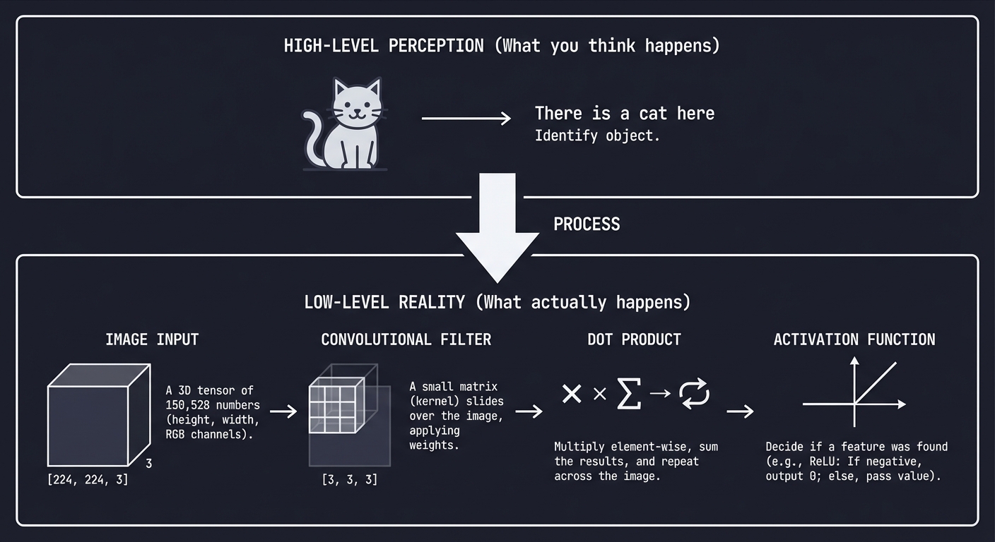
Every vision system, from a simple QR code scanner to a humanoid robot, operates on these fundamental steps.
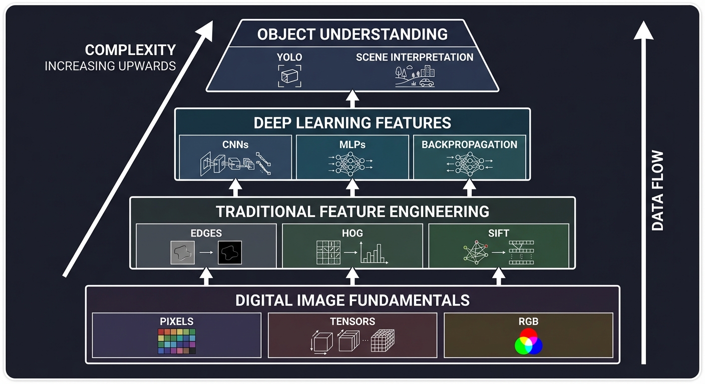
The Computer Vision Hierarchy: From Pixels to Logic
┌─────────────────────────────────────────────────────────────────┐
│              Object Understanding (Logic/Scene)                  │
│  ← "What is happening in this video?" (YOLO, Action Recognition)│
├─────────────────────────────────────────────────────────────────┤
│              Deep Learning Features (The "Black Box")            │
│  ← CNNs, MLPs, Backpropagation, Learned Filters                 │
├─────────────────────────────────────────────────────────────────┤
│              Traditional Feature Engineering                     │
│  ← HOG, SIFT, Canny Edges, Sobel Kernels                        │
├─────────────────────────────────────────────────────────────────┤
│              Digital Image Fundamentals (Raw Data)               │
│  ← Pixels, Tensors, RGB/HSV, Matrix Arithmetic                  │
└─────────────────────────────────────────────────────────────────┘
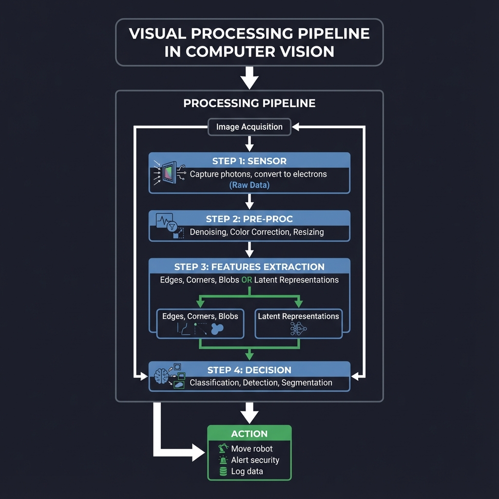
The Visual Processing Pipeline: From Pixels to Perception
┌─────────────────────────────────────────────────────────────────┐
│                       Image Acquisition                          │
│  ┌─────────┐                                                    │
│  │ Sensor  │  ← Capture photons, convert to electrons (Raw Data) │
│  └────┬────┘                                                    │
│       │                                                          │
│  ┌────┴────┐                                                    │
│  │ Pre-Proc│  ← Denoising, Color Correction, Resizing           │
│  └────┬────┘                                                    │
│       │                                                          │
│  ┌────┴────┐                                                    │
│  │ Features│  ← Edges, Corners, Blobs (Traditional) OR           │
│  │ Extraction  ← Latent Representations (Deep Learning)         │
│  └────┬────┘                                                    │
│       │                                                          │
│  ┌────┴────┐                                                    │
│  │ Decision│  ← Classification, Detection, Segmentation         │
│  └────┬────┘                                                    │
└───────┼─────────────────────────────────────────────────────────┘
        │
┌───────┴─────────────────────────────────────────────────────────┐
│       Action     ← Move robot, Alert security, Log data         │
└─────────────────────────────────────────────────────────────────┘
When you write cv2.imread(), you’re not just “opening a file”—you’re loading a digital canvas of numerical intensities into memory.
Core Concept Analysis
1. Image Representation: The Numerical Grid
At its core, a digital image is a grid of numbers. For color images, we use 3 channels: Red, Green, and Blue.
(0,0) ┌───┬───┬───┬───┐
      │R,G│R,G│R,G│...│
      │,B │,B │,B │   │
      ├───┼───┼───┼───┤
      │R,G│R,G│R,G│...│
      │,B │,B │,B │   │
      └───┴───┴───┴───┘ (Width, Height)

Each channel value is usually 8-bit (0-255).
Total Numbers = Width * Height * 3
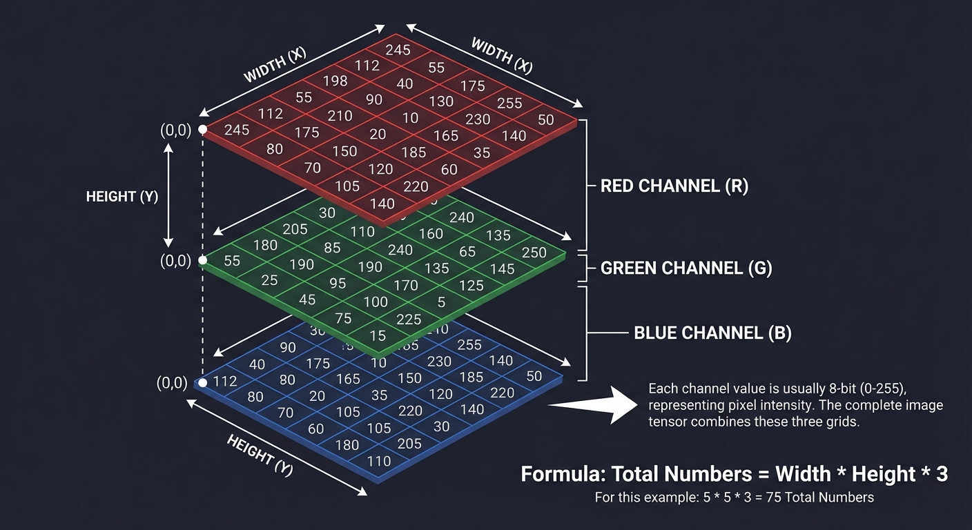
Key insight: Computers don’t see “shapes.” They see gradients (differences between numbers). A “vertical edge” is just a column of numbers where the values on the left are significantly higher than the values on the right.
2. Convolution: The Sliding Window
Convolution is the mathematical heart of vision. It involves a Kernel (a small matrix) sliding across the Input Image.
Input Image (5x5)            Kernel (3x3)           Output Map (3x3)
┌───┬───┬───┬───┬───┐        ┌───┬───┬───┐          ┌───┬───┬───┐
│ 1 │ 1 │ 1 │ 0 │ 0 │        │ 1 │ 0 │-1 │          │ 4 │ 3 │ 4 │
├───┼───┼───┼───┼───┤        ├───┼───┼───┤          ├───┼───┼───┤
│ 0 │ 1 │ 1 │ 1 │ 0 │    *   │ 1 │ 0 │-1 │    =     │ 2 │ 4 │ 3 │
├───┼───┼───┼───┼───┤        ├───┼───┼───┤          ├───┼───┼───┤
│ 0 │ 0 │ 1 │ 1 │ 1 │        │ 1 │ 0 │-1 │          │ 2 │ 3 │ 4 │
├───┼───┼───┼───┼───┤        └───┴───┴───┘          └───┴───┴───┘
│ ...
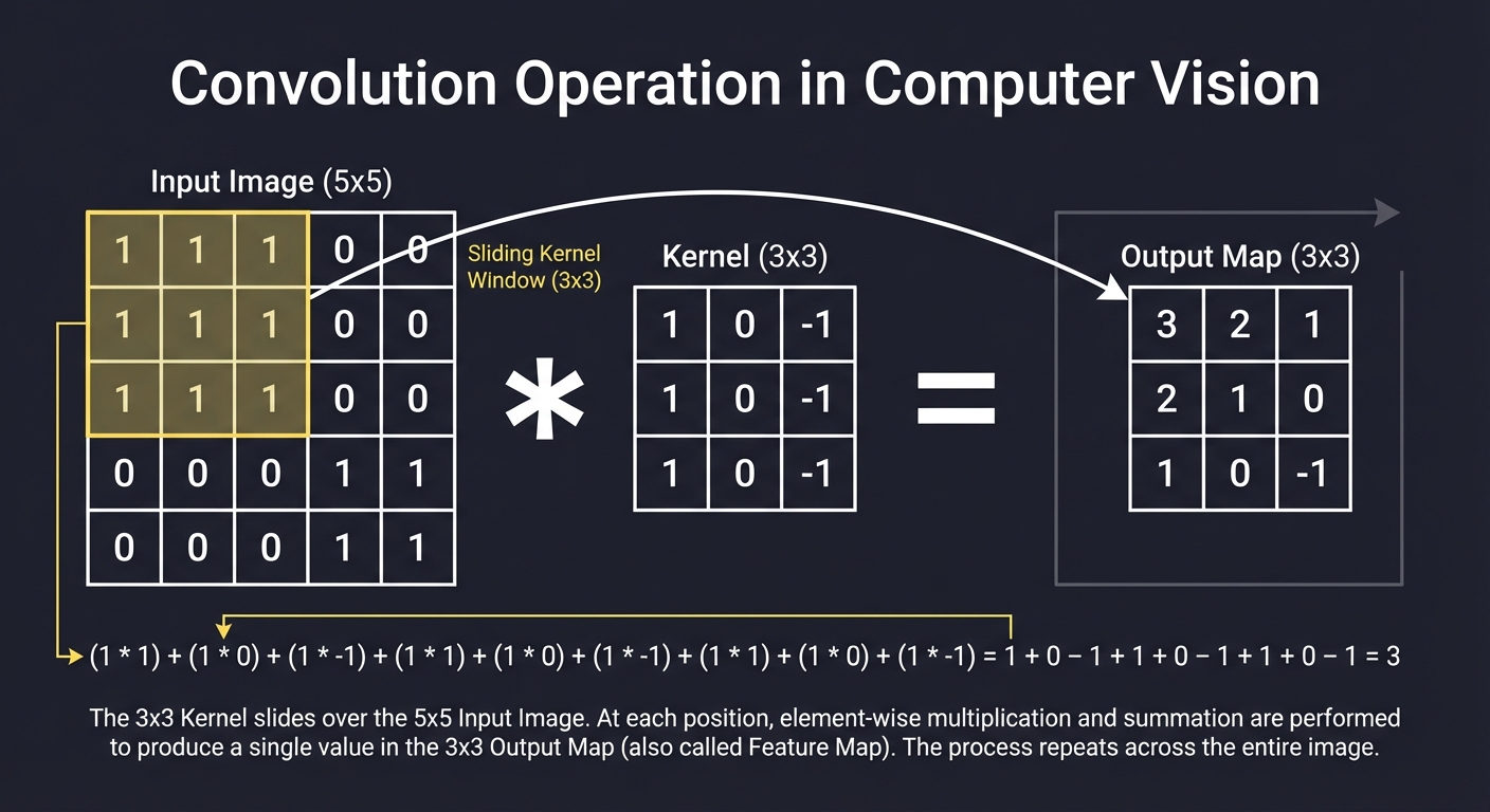
- Filters: Detect specific patterns. A Sobel filter detects edges; a Gaussian filter blurs noise.
- Padding: Adding borders (usually zeros) so the kernel can reach the edges of the image.
- Stride: How many pixels the window jumps each step.
3. Feature Extraction (Traditional vs. Deep)
Traditional (Hand-Crafted)
Engineers used math to define what a “pedestrian” looks like using:
- HOG (Histogram of Oriented Gradients): Counts occurrences of gradient orientation in localized portions of an image.
- SIFT/SURF: Finds “blobs” that don’t change when you rotate or scale the image.
Deep Learning (Learned)
CNNs (Convolutional Neural Networks) don’t wait for humans to define features. They learn the filters through backpropagation.
Layer 1: Detects raw edges (low-level)
Layer 2: Combines edges into shapes (mid-level)
Layer 3: Combines shapes into object parts (high-level)
Layer 4: Combines parts into final categories (Cat, Dog, etc.)
4. Object Detection & YOLO
Classification says “This is a cat.” Detection says “This is a cat, and it is at these coordinates (x, y, w, h).”
YOLO (You Only Look Once) radicalized detection by treating it as a single regression problem.
1. Divide image into an S x S grid.
2. Each cell predicts B bounding boxes.
3. Each box has a confidence score.
4. Each cell predicts class probabilities.
Instead of looking at thousands of “region proposals,” YOLO looks at the entire image once, making it fast enough for real-time video.
5. Non-Maximum Suppression (NMS)
When a model detects an object, it often outputs multiple boxes for the same thing.
Predicted Boxes:       After NMS:
   ┌───┐                  ┌───┐
 ┌─┼───┼─┐                │   │
 │ └───┘ │        →       │   │
 └───────┘                └───┘
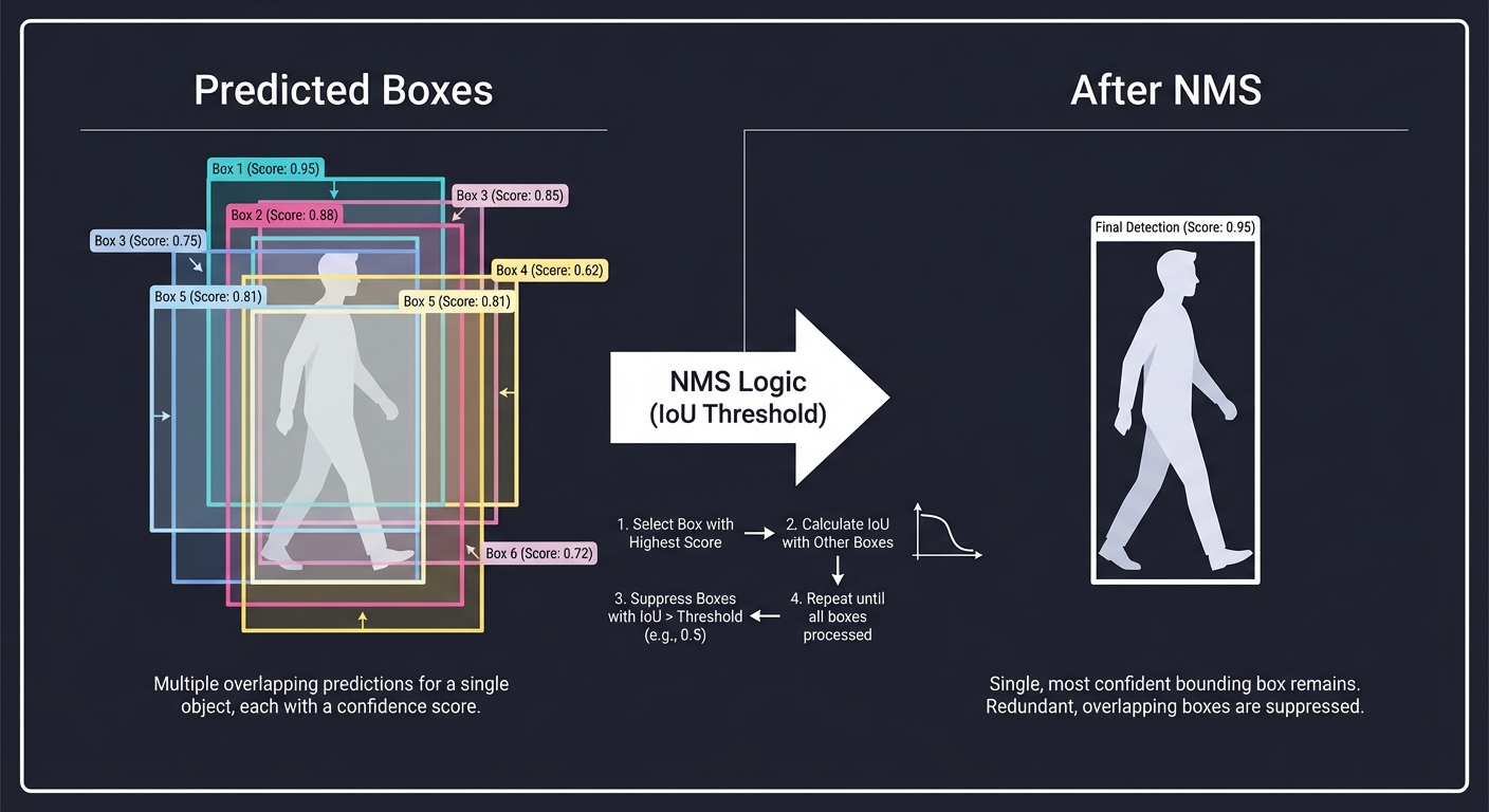
Key insight: We calculate IoU (Intersection over Union) between boxes. If two boxes overlap heavily, we keep the one with the highest confidence and “suppress” the others.
6. Neural Networks: The Learning Engine
While traditional CV uses hand-crafted filters, Deep Learning uses Backpropagation to learn the best filters for a specific task.
Input x -> [ Weights W ] -> Prediction y -> Loss(y, target)
               ↑                               |
               └-------[ Gradient Flow ]-------┘
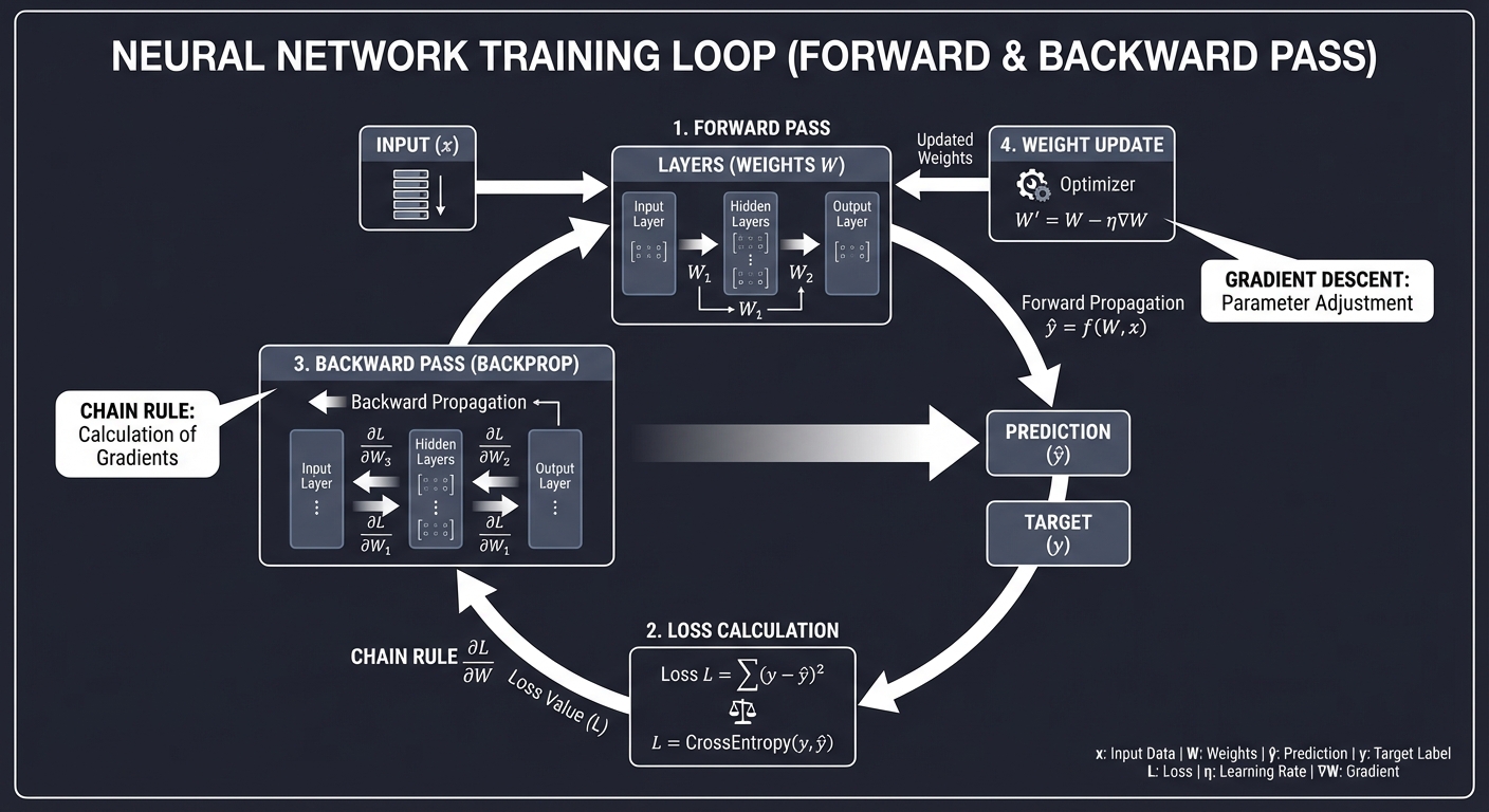
- Weights: The values inside the filters/kernels.
- Backpropagation: Calculating how much each weight contributed to the error (using the Chain Rule).
- Optimization: Nudging the weights in the opposite direction of the gradient to reduce error.
Concept Summary Table
| Concept Cluster | What You Need to Internalize |
|---|---|
| Tensors as Images | Images are multi-dimensional arrays. Shape (H, W, C) is standard. |
| Convolution Math | Element-wise multiplication followed by summation. The “sliding window” logic. |
| Gradient Flow | How pixel differences define edges and shapes. |
| Backpropagation | How a network learns to adjust its filters to minimize error. |
| Object Detection | Bounding box regression vs image classification. |
| Real-time Pipeline | Grid systems, anchors, and NMS for speed. |
| Transfer Learning | Using a model trained on ImageNet and “fine-tuning” it for your specific task. |
Deep Dive Reading by Concept
This section maps each concept from above to specific book chapters for deeper understanding. Read these before or alongside the projects to build strong mental models.
Image Fundamentals & Processing
| Concept | Book & Chapter |
|---|---|
| Digital Image Basics | Digital Image Processing (Gonzalez & Woods) — Ch. 2: “Digital Image Fundamentals” |
| Spatial Filtering & Convolution | Digital Image Processing (Gonzalez & Woods) — Ch. 3: “Intensity Transformations and Spatial Filtering” |
| Color Models (RGB, HSV, YCbCr) | Digital Image Processing (Gonzalez & Woods) — Ch. 6: “Color Image Processing” |
| Frequency Domain Processing | Digital Image Processing (Gonzalez & Woods) — Ch. 4: “Filtering in the Frequency Domain” |
Traditional Computer Vision
| Concept | Book & Chapter |
|---|---|
| Feature Detection (SIFT, HOG) | Computer Vision: Algorithms and Applications (Szeliski) — Ch. 4: “Feature detection and matching” |
| Edge Detection (Sobel, Canny) | Computer Vision: Algorithms and Applications (Szeliski) — Ch. 4.2: “Edges” |
| Image Segmentation | Computer Vision: Algorithms and Applications (Szeliski) — Ch. 5: “Segmentation” |
Deep Learning & CNNs
| Concept | Book & Chapter |
|---|---|
| Neural Network Basics | Hands-On Machine Learning (Géron) — Ch. 10: “Introduction to Artificial Neural Networks with Keras” |
| CNN Architectures | Hands-On Machine Learning (Géron) — Ch. 14: “Deep Computer Vision Using Convolutional Neural Networks” |
| Convolutional Mechanics | Deep Learning (Goodfellow) — Ch. 9: “Convolutional Networks” |
| Optimization for Training | Deep Learning (Goodfellow) — Ch. 8: “Optimization for Training Deep Models” |
Object Detection (YOLO, etc.)
| Concept | Book & Chapter |
|---|---|
| Object Detection Fundamentals | Hands-On Machine Learning (Géron) — Ch. 15: “Processing Sequences Using RNNs and CNNs” (Section on Detection) |
| YOLO Architecture | YOLOv1 Paper: “You Only Look Once: Unified, Real-Time Object Detection” (Redmon et al.) |
| Semantic Segmentation | Hands-On Machine Learning (Géron) — Ch. 14 (Section on Segmentation) |
Project 1: Raw Image Viewer and Manipulator
- Main Programming Language: Python
- Alternative Programming Languages: C++, Rust, Go
- Coolness Level: Level 2: Practical but Forgettable
- Business Potential: 1. The “Resume Gold”
- Difficulty: Level 1: Beginner
- Knowledge Area: Image Representation, Basic I/O
- Software or Tool: Pillow (PIL Fork) or OpenCV
- Main Book: “Digital Image Processing” by Gonzalez & Woods
What you’ll build: A tool that loads images (PNG/JPG), displays them, and performs pixel-level manipulations like grayscale conversion and channel extraction (R, G, or B).
Why it teaches CV: It forces you to see an image as a 2D/3D array of numbers. You’ll understand how simple arithmetic on these numbers changes what we see.
Core challenges you’ll face:
- Pixel-level access: Directly manipulating RGB channels.
- Color space conversion: Implementing the weighted RGB-to-Grayscale formula.
- NumPy integration: Learning to treat images as high-performance arrays.
Real World Outcome
You’ll have a high-performance CLI tool that processes images without using high-level filter libraries. You’ll be able to “dissect” an image into its constituent colors and intensities.
Example Output:
$ python image_tool.py --input photo.jpg --mode channel --param Red --output red_channel.png
Loading photo.jpg (1920x1080)...
Extracting RED channel...
Zeroing out GREEN and BLUE channels...
Saved: red_channel.png

$ python image_tool.py --input photo.jpg --mode grayscale --output out.png
Applying weighted average (Luminance) to 2,073,600 pixels...
Saved: out.png
The Core Question You’re Answering
“What IS a digital image? Is it a file, or is it just a big array of numbers we choose to interpret as light?”
Before you write any code, realize that every “AI” or “Vision” algorithm eventually has to look at these raw numbers. If you can’t manipulate the numbers, you can’t build the AI.
Concepts You Must Understand First
Stop and research these before coding:
- The RGB Color Model
- How are colors represented by three numbers?
- What is the bit-depth of a standard JPEG?
- Book Reference: “Digital Image Processing” Ch. 6.1
- NumPy Array Slicing
- How do you access all the “Red” values at once without a
forloop? - What is the difference between a shallow copy and a deep copy of an image?
- Book Reference: NumPy Documentation (Indexing and Slicing)
- How do you access all the “Red” values at once without a
- Luminance and Human Perception
- Why do we use
0.299R + 0.587G + 0.114Bfor grayscale instead of(R+G+B)/3? - Which color are humans most sensitive to?
- Why do we use
Questions to Guide Your Design
Before implementing, think through these:
- Memory Layout
- If an image is 100x100 pixels, how many numbers are in its RGB array? (30,000)
- Is it stored as
[R,G,B, R,G,B...]or[[R...],[G...],[B...]]?
- Overflow Handling
- If you add 10 to every pixel to make it brighter, what happens if a pixel was already at 250?
- How do you “clamp” values to the 0-255 range?
- Efficiency
- Why is iterating through pixels with a Python
forloop so slow compared to NumPy operations?
- Why is iterating through pixels with a Python
Thinking Exercise
The Weighted Average
Look at these two RGB pixels:
(200, 50, 50)- Very Red(50, 200, 50)- Very Green
If you take a simple average (R+G+B)/3, they might look the same intensity. But the human eye is much more sensitive to green than red or blue.
- Implement both methods: Simple Average vs. Luminance.
- Compare the results on a colorful photo. Which looks more “natural”?
The Interview Questions They’ll Ask
Prepare to answer these:
- “What is the shape of a 3-channel color image tensor in NumPy?”
- “Why is a grayscale image often preferred for edge detection?”
- “Explain the difference between additive (RGB) and subtractive (CMYK) color models.”
- “How would you implement a ‘brightness’ filter using only matrix arithmetic?”
Hints in Layers
Hint 1: Loading
Use Pillow’s Image.open() and then convert it to a NumPy array using img_array = np.array(img).
Hint 2: Manipulation
A 3-channel image is an array of shape (Height, Width, 3). Accessing arr[:, :, 0] gives you the Red intensity for ALL pixels at once.
Hint 3: Logic
To make the whole image Red, you would create a copy of the image and set copy_arr[:, :, 1] = 0 (Green) and copy_arr[:, :, 2] = 0 (Blue).
Books That Will Help
| Topic | Book | Chapter |
|---|---|---|
| Image Representation | “Digital Image Processing” | Ch. 2.1-2.4 |
| Color Spaces | “Digital Image Processing” | Ch. 6.1-6.2 |
| Array Manipulation | “Hands-On Machine Learning” | Appendix C (NumPy) |
| Performance in Python | “High Performance Python” | Ch. 6 (Matrix and Vector Computation) |
Project 2: Custom Convolutional Filters from Scratch
- Main Programming Language: Python
- Alternative Programming Languages: C++, Rust
- Coolness Level: Level 3: Genuinely Clever
- Business Potential: 1. The “Resume Gold”
- Difficulty: Level 2: Intermediate
- Knowledge Area: Image Processing, Linear Algebra
- Software or Tool: NumPy
- Main Book: “Digital Image Processing” by Gonzalez & Woods
What you’ll build: A program that applies convolutional kernels (Blur, Sharpen, Edge Detect) by sliding a small matrix over an image and calculating weighted sums.
Why it teaches CV: This is the absolute foundation of Convolutional Neural Networks (CNNs). Before the “Deep” part, there was just convolution.
Core challenges you’ll face:
- Implementation of sliding window: Coding the loops to move the kernel across the image.
- Padding: Deciding what to do when the kernel “falls off” the edge of the image.
- Normalization: Ensuring pixel values don’t explode past 255.
Real World Outcome
You’ll be able to blur, sharpen, and detect edges in images using your own math, not a “black box” function. This tool is effectively a manual version of a single layer in a CNN.
Example Output:
$ python convolution_tool.py --input dog.png --kernel blur_3x3 --output blurred.png
Loading 512x512 image...
Kernel:
[[0.11, 0.11, 0.11],
 [0.11, 0.11, 0.11],
 [0.11, 0.11, 0.11]]
Processing... Handling boundaries with Reflective Padding.
Saved: blurred.png

$ python convolution_tool.py --input dog.png --kernel sobel_v --output vertical_edges.png
Applying Vertical Sobel Filter...
Detected intensity gradients.
Saved: vertical_edges.png
The Core Question You’re Answering
“How can a tiny 3x3 matrix of numbers ‘understand’ the difference between a blurry background and a sharp edge?”
The magic of convolution is that it looks at a pixel in context of its neighbors. You’re moving from pixel-level thinking to neighborhood-level thinking.
Concepts You Must Understand First
Stop and research these before coding:
- The Convolution Operation
- What is a “Kernel” or “Filter”?
- How does element-wise multiplication and summation work in a sliding window?
- Book Reference: “Digital Image Processing” Ch. 3.4.1
- Padding Strategies
- What is “Zero Padding” vs. “Reflective Padding”?
- Why do we need padding to keep the output image the same size as the input?
- Spatial Frequency
- Why does a “smoothing” kernel (like Mean or Gaussian) have all positive numbers?
- Why does an “edge” kernel (like Sobel) have both positive and negative numbers?
Questions to Guide Your Design
Before implementing, think through these:
- Loop Structure
- You need nested loops for Image Width/Height and Kernel Width/Height. How can you optimize this?
- Boundary Conditions
- What happens when you try to calculate the output for the pixel at
(0,0)with a 3x3 kernel?
- What happens when you try to calculate the output for the pixel at
- Normalization
- If your kernel values sum to more than 1, the image will get brighter. If they sum to 0 (like Sobel), how do you handle negative output values? (Absolute value or clipping?)
Thinking Exercise
The Kernel’s Secret
Imagine a 3x3 kernel that is all 0s except for a 1 in the center:
[0, 0, 0]
[0, 1, 0]
[0, 0, 0]
What happens to the image when you convolve it with this kernel? (Identity transformation)
Now imagine this kernel (Mean Blur):
[1/9, 1/9, 1/9]
[1/9, 1/9, 1/9]
[1/9, 1/9, 1/9]
What visual effect does this produce? Why do we divide by 9?
The Interview Questions They’ll Ask
Prepare to answer these:
- “What is the difference between convolution and cross-correlation in image processing?”
- “Why are kernels almost always odd-sized (3x3, 5x5)?”
- “Explain how the Sobel filter approximates the first derivative of the image.”
- “What are separable filters and why do they matter for performance?”
Hints in Layers
Hint 1: The Core Loop
Iterate i from 0 to ImageHeight - KernelHeight and j from 0 to ImageWidth - KernelWidth.
Hint 2: Sub-matrix Selection
For each (i, j), extract the sub-image: sub_img = input_img[i:i+K, j:j+K]. Then use np.sum(sub_img * kernel).
Hint 3: Use np.pad
Instead of manually handling edges in the loop, use np.pad(image, pad_width=1, mode='constant') before starting the loop.
Books That Will Help
| Topic | Book | Chapter |
|---|---|---|
| Spatial Filtering | “Digital Image Processing” | Ch. 3.4-3.6 |
| Convolutions & Kernels | “Computer Vision: Algorithms and Applications” | Ch. 3.2 |
| Convolutional Layers | “Deep Learning” | Ch. 9 |
Project 3: Canny Edge Detector from Scratch
- Main Programming Language: Python
- Alternative Programming Languages: C++, Rust
- Coolness Level: Level 4: Hardcore Tech Flex
- Business Potential: 1. The “Resume Gold”
- Difficulty: Level 3: Advanced
- Knowledge Area: Feature Extraction, Algorithms
- Software or Tool: NumPy
- Main Book: “Computer Vision: Algorithms and Applications” by Szeliski
What you’ll build: A full implementation of the Canny algorithm: Noise reduction, Gradient calculation, Non-maximum suppression, and Hysteresis thresholding.
Why it teaches CV: It’s a multi-stage pipeline. You’ll learn how to transform noisy pixel data into clean, mathematical lines representing object boundaries.
Core challenges you’ll face:
- Gradient Direction: Calculating angles and mapping them to 8-connected neighbors.
- Hysteresis: Implementing the recursive logic to connect weak edges to strong ones.
- Precision: Managing floating-point gradients vs integer pixel outputs.
Real World Outcome
A tool that produces clean, 1-pixel wide line drawings (edge maps) from noisy photos. This is the first step in object recognition for many classical systems.
Example Output:
$ python canny.py --input car.jpg --low 50 --high 150 --output sketch.png
Step 1: Gaussian Blur... Done.
Step 2: Sobel Gradients (Magnitude & Direction)... Done.
Step 3: Non-Max Suppression (Thinning)... Done.
Step 4: Hysteresis Thresholding (Connecting)... Done.
Result: 42,102 edge pixels detected.
Saved: sketch.png
The Core Question You’re Answering
“In a world of noisy, blurry pixels, how can a computer decide exactly where an object starts and ends?”
Canny isn’t just one formula; it’s a decision-making process. You’ll understand why “smoothing” is the first step in almost all vision algorithms.
Concepts You Must Understand First
Stop and research these before coding:
- Gaussian Smoothing
- Why do we blur before finding edges? (To remove noise that looks like tiny edges)
- Book Reference: “Digital Image Processing” Ch. 3.5.2
- Image Gradients (Magnitude & Direction)
- How do you use
GxandGyto find the angle of an edge? - What does it mean for an edge to be at 45 degrees?
- How do you use
- Non-Maximum Suppression (NMS)
- If an edge is 3 pixels wide, how do you keep only the sharpest “peak” pixel?
- Double Thresholding & Hysteresis
- What is a “strong” edge vs. a “weak” edge?
- How do you “trace” an edge through a grid?
Questions to Guide Your Design
Before implementing, think through these:
- Angle Quantization
- Computers work in a grid. How do you map a continuous angle (e.g., 22.5 degrees) to one of the 8 neighbors?
- NMS Comparison
- For a pixel at
(x, y)with a vertical gradient, which two neighbors do you compare it against?
- For a pixel at
- Recursive Tracing
- Hysteresis requires checking neighbors of weak edges. Should you use recursion (DFS) or a queue (BFS)?
Thinking Exercise
The Thinning Problem
Draw a 5x5 grid of numbers where a “diagonal edge” is represented by a ramp of values (e.g., 0, 50, 100, 150, 200).
- Calculate the gradient magnitude at each pixel.
- Now, pick the middle pixel and its two neighbors in the direction of the gradient. Which one is the maximum?
- If you keep only the maximum, what does your grid look like now? (This is NMS in action).
The Interview Questions They’ll Ask
Prepare to answer these:
- “What are the five steps of the Canny Edge Detection algorithm?”
- “Why is Non-Maximum Suppression (NMS) necessary?”
- “Explain how Hysteresis helps in detecting weak edges.”
- “How does the ‘sigma’ parameter of the Gaussian blur affect the final edge map?”
Hints in Layers
Hint 1: Reuse Project 2 Your Canny implementation should use your convolution code from Project 2 for the Gaussian blur and Sobel steps.
Hint 2: Angle Mapping Map your angles to four groups: 0°, 45°, 90°, and 135°.
- 0°: Check Left/Right neighbors.
- 90°: Check Up/Down neighbors.
Hint 3: Hysteresis Logic Iterate through all pixels. If a pixel is “Strong” (> High Threshold), mark it as an edge. Then recursively (or using a stack) check its “Weak” neighbors (between Low and High) and mark them too.
Books That Will Help
| Topic | Book | Chapter |
|---|---|---|
| Image Gradients | “Digital Image Processing” | Ch. 10.1-10.2 |
| Canny Algorithm | “Computer Vision: Algorithms and Applications” | Ch. 4.2 |
| Feature Detection | “Introductory Techniques for 3D Computer Vision” | Ch. 4 |
Project 4: Simple Object Classifier (HOG + SVM)
- Main Programming Language: Python
- Alternative Programming Languages: C++, R
- Coolness Level: Level 3: Genuinely Clever
- Business Potential: 1. The “Resume Gold”
- Difficulty: Level 3: Advanced
- Knowledge Area: Classical Machine Learning, Feature Engineering
- Software or Tool: Scikit-learn, NumPy
- Main Book: “Computer Vision: Algorithms and Applications” by Szeliski
What you’ll build: A system that extracts “Histogram of Oriented Gradients” (HOG) features and uses a Support Vector Machine (SVM) to classify images (e.g., Pedestrian vs No Pedestrian).
Why it teaches CV: You’ll learn the difference between “raw pixels” and “features.” You’ll see how describing the shape of an object (via edge histograms) is more robust than looking at pixel colors.
Core challenges you’ll face:
- Feature Vector Construction: Flattening image summaries into a format a machine learning model can read.
- Dataset Preparation: Balancing classes and normalizing images.
- Parameter Tuning: Finding the right HOG cell size and SVM kernel.
Real World Outcome
You’ll be able to feed a new image to your script and have it correctly label it based on training data. This is how early facial recognition and pedestrian detection systems worked before CNNs.
Example Output:
$ python predict.py --model pedestrian_model.pkl --image street.jpg
Extracting HOG features (Vector size: 3780)...
Running SVM Inference...
Result: [PEDESTRIAN] (Confidence: 0.89)

$ python predict.py --model pedestrian_model.pkl --image park_bench.jpg
Result: [NO PEDESTRIAN] (Confidence: 0.95)
The Core Question You’re Answering
“How can we describe the ‘essence’ of a shape without looking at raw pixel colors, which change based on lighting?”
HOG focuses on the distribution of directions of gradients. It captures the “silhouette” of an object.
Concepts You Must Understand First
Stop and research these before coding:
- Histogram of Oriented Gradients (HOG)
- What is a “cell” and a “block” in HOG?
- How does normalization across blocks help with lighting changes?
- Book Reference: “Computer Vision” (Szeliski) Ch. 14.1.1
- Support Vector Machines (SVM)
- How does an SVM find the “widest margin” between classes?
- What is a “Hyperplane”?
- Book Reference: “Hands-On Machine Learning” Ch. 5
- Feature Vectors
- How do you turn a 2D grid of histograms into a 1D vector for a classifier?
Questions to Guide Your Design
Before implementing, think through these:
- Scale Invariance
- If a pedestrian is far away, they are smaller. How do you ensure your HOG extractor can see them? (Image pyramids or resizing).
- Gradient vs. Color
- Why would a HOG detector work even if the pedestrian is wearing a green shirt or a red shirt?
- Training Data
- How many “Negative” (non-pedestrian) images do you need to train a robust model?
Thinking Exercise
The Orientation Bin
Imagine a 8x8 patch of pixels representing the top-left corner of a box.
- The gradients are mostly pointing at 45° and 90°.
- If you have 9 “bins” (0°, 20°, 40°… 160°), which bins will have the highest values?
- How does this “histogram” represent the shape of that corner?
The Interview Questions They’ll Ask
Prepare to answer these:
- “Why use HOG instead of just feeding raw pixels into a classifier?”
- “Explain the role of ‘block normalization’ in HOG.”
- “How does a linear SVM handle non-linear data? (Hint: Kernels)”
- “What are ‘Hard Negatives’ and why are they important in object detection training?”
Hints in Layers
Hint 1: Use skimage
While you should understand the math, start with skimage.feature.hog to extract features quickly.
Hint 2: Image Pyramids For detection in a large image, resize the image at multiple scales and run your “sliding window” classifier on each scale.
Hint 3: SVM Kernel Start with a Linear kernel. If your accuracy is low, try an RBF (Radial Basis Function) kernel, but be aware of the performance cost.
Books That Will Help
| Topic | Book | Chapter |
|---|---|---|
| HOG Descriptor | “Computer Vision: Algorithms and Applications” | Ch. 14.1 |
| SVM Foundations | “Hands-On Machine Learning” | Ch. 5 |
| Feature Engineering | “The Elements of Statistical Learning” | Ch. 12 |
Project 5: MLP from Scratch (MNIST)
- Main Programming Language: Python
- Alternative Programming Languages: C++, JavaScript
- Coolness Level: Level 3: Genuinely Clever
- Business Potential: 1. The “Resume Gold”
- Difficulty: Level 2: Intermediate
- Knowledge Area: Neural Networks, Calculus
- Software or Tool: NumPy
- Main Book: “Hands-On Machine Learning” by Géron
What you’ll build: A multi-layer perceptron (neural network) that recognizes handwritten digits. You must implement the forward pass, backpropagation, and weight updates using only NumPy.
Why it teaches CV: It demystifies the “learning” part of AI. You’ll see exactly how the network adjusts its “weights” to see the difference between a 3 and an 8.
Core challenges you’ll face:
- The Chain Rule: Implementing the calculus of backpropagation manually.
- Activation Functions: Writing Sigmoid, ReLU, and Softmax from scratch.
- Matrix Dimensions: Ensuring that matrix multiplications align at every layer.
Real World Outcome
A neural network trained on 60,000 images that can accurately predict the number in a hand-drawn digit with >95% accuracy.
Example Output:
$ python train_mlp.py --epochs 10
Epoch 1: Loss: 2.30, Accuracy: 12%
...
Epoch 10: Loss: 0.15, Accuracy: 96%
Training Complete. Weights saved to model.npz

$ python test_mlp.py --image my_digit.png
Neural Network Input (28x28 flattened to 784)...
Inference...
Predicted Digit: [3] (Confidence: 0.992)
The Core Question You’re Answering
“How can a bunch of random numbers (weights) eventually learn to ‘read’ human handwriting?”
This project answers that. It’s not magic; it’s iterative optimization through calculus.
Concepts You Must Understand First
Stop and research these before coding:
- Forward Propagation
- How do inputs, weights, and biases combine to produce an output?
Z = W * X + b
- Backpropagation (The Chain Rule)
- How do you calculate the gradient of the error with respect to a weight in the first layer?
- Book Reference: “Deep Learning” (Goodfellow) Ch. 6.5
- Loss Functions (Cross-Entropy)
- Why is “Mean Squared Error” bad for classification?
- How does Cross-Entropy measure the “distance” between probability distributions?
- Stochastic Gradient Descent (SGD)
- How do you move the weights “downhill” to find the minimum error?
Questions to Guide Your Design
Before implementing, think through these:
- Weight Initialization
- If you start all weights at 0, will the network learn? (Spoiler: No). Why?
- Hidden Layer Count
- How many neurons do you need to distinguish between 10 digits?
- Softmax Output
- How do you ensure your 10 output neurons sum to 1.0?
Thinking Exercise
Trace a Single Update
Imagine a tiny network: 1 input, 1 hidden neuron (ReLU), 1 output.
- Input
x = 1.0, Targety = 0.0. - Current weights
w1 = 0.5,w2 = 0.5. - Calculate the forward pass.
- Calculate the error.
- Use a learning rate of
0.1and calculate the neww1andw2after one backprop step.
The Interview Questions They’ll Ask
Prepare to answer these:
- “Explain the Vanishing Gradient problem.”
- “Why do we use ReLU instead of Sigmoid in hidden layers?”
- “What is ‘Overfitting’ and how can you detect it during training?”
- “Describe the difference between Batch, Mini-batch, and Stochastic Gradient Descent.”
Hints in Layers
Hint 1: Matrix Shape Verification
Always print X.shape, W.shape, and b.shape before a multiplication. If (N, M) doesn’t meet (M, P), the code will crash.
Hint 2: Softmax Stability
When calculating Softmax, subtract the maximum value from your vector before exponentiating to avoid “Numerical Explosion” (inf).
Hint 3: Derivative of ReLU
The derivative is 1 if x > 0 and 0 otherwise. It’s much simpler than Sigmoid’s derivative.
Books That Will Help
| Topic | Book | Chapter |
|---|---|---|
| Neural Network Intro | “Hands-On Machine Learning” | Ch. 10 |
| Deep Learning Theory | “Deep Learning” (Goodfellow) | Ch. 6 |
| Backpropagation Math | “Calculus” (Any textbook) | Chain Rule |
| MNIST Dataset Handling | “Neural Networks and Deep Learning” | Ch. 1 |
Project 6: First CNN from Scratch
- Main Programming Language: Python
- Alternative Programming Languages: C++
- Coolness Level: Level 4: Hardcore Tech Flex
- Business Potential: 1. The “Resume Gold”
- Difficulty: Level 4: Expert
- Knowledge Area: Deep Learning, Architecture
- Software or Tool: NumPy
- Main Book: “Deep Learning” by Goodfellow
What you’ll build: A Convolutional Neural Network (Conv -> ReLU -> Pool -> FC) from scratch. You’ll implement the forward and backward passes for 4D tensors (Batch, Channel, Height, Width).
Why it teaches CV: This combines Project 2 (Convolution) with Project 5 (Learning). You’ll understand why CNNs are so much better for images than regular MLPs.
Core challenges you’ll face:
- Backprop through Convolution: This is significantly harder than backprop through linear layers.
- Max Pooling Switch: Tracking indices during the forward pass so you know where to send gradients during the backward pass.
- Dimensionality: Managing the change in image size as it moves through the layers.
Real World Outcome
A specialized neural network that achieves >98% accuracy on MNIST and can generalize to complex images like those in CIFAR-10. You will have implemented the code that powers nearly every visual AI today.
Example Output:
$ python train_cnn.py --arch "C32-P2-C64-P2-F128"
Conv Layer 1: [Batch, 32, 28, 28]
Pool Layer 1: [Batch, 32, 14, 14]
...
Epoch 5: Val Accuracy: 99.1%
The Core Question You’re Answering
“Why is a convolutional layer better for images than a ‘flat’ linear layer?”
The answer lies in Spatial Locality. CNNs assume that pixels close to each other are related. Flat layers forget where pixels were located.
Concepts You Must Understand First
Stop and research these before coding:
- The Conv2D Backward Pass
- How do gradients flow through a filter? (It’s actually another convolution!)
- Book Reference: “Deep Learning” (Goodfellow) Ch. 9.5
- Pooling (Max vs. Average)
- Why does pooling provide “Translation Invariance”?
- How do you backprop through a “Max” operation? (Only the winner gets the gradient).
- Receptive Fields
- How much of the original image does a single neuron in Layer 3 “see”?
Questions to Guide Your Design
Before implementing, think through these:
- Feature Map Count
- Why do we usually increase the number of channels (filters) as we go deeper into the network?
- Parameter Sharing
- How many parameters are in a 3x3 filter compared to a fully connected layer for a 224x224 image?
- Stride and Padding
- How do these parameters affect the “resolution” of your feature maps?
Thinking Exercise
The translation test
Imagine an image of a “1”. If you shift that “1” five pixels to the right:
- Does an MLP see the same input? (No, every pixel changed its index).
- Does a CNN see the same feature? (Yes, the filter will simply detect the “1” at a different stride step).
- Explain why this makes CNNs robust.
The Interview Questions They’ll Ask
Prepare to answer these:
- “Explain the ‘im2col’ trick for speeding up convolutions.”
- “What is a 1x1 convolution and why is it useful?”
- “Explain the difference between a Filter and a Kernel in the context of CNNs.”
- “Why do we typically use Max Pooling instead of Average Pooling for vision?”
Hints in Layers
Hint 1: Start with 1 channel Implement the forward/backward pass for a single-channel grayscale image first. Adding multiple channels is just an extra dimension in your summation.
Hint 2: Tracking Max Indices
In your forward pass for MaxPool, save a “mask” array that stores the location of the maximum value. You’ll need this to place the gradients correctly during backward.
Hint 3: Use im2col
Implementing convolution as 4 nested loops is too slow for training. Research how to turn the image into a large matrix (im2col) so you can use np.dot for the whole layer at once.
Books That Will Help
| Topic | Book | Chapter |
|---|---|---|
| CNN Architecture | “Hands-On Machine Learning” | Ch. 14 |
| Conv Net Mechanics | “Deep Learning” (Goodfellow) | Ch. 9 |
| Optimization | “Efficient Processing of Deep Neural Networks” | Ch. 3 |
Project 7: Non-Maximum Suppression (NMS)
- Main Programming Language: Python
- Alternative Programming Languages: C++, Rust, Go
- Coolness Level: Level 3: Genuinely Clever
- Business Potential: 1. The “Resume Gold”
- Difficulty: Level 2: Intermediate
- Knowledge Area: Object Detection, Geometry
- Software or Tool: NumPy
- Main Book: “Computer Vision” (Szeliski)
What you’ll build: A logic module that takes hundreds of overlapping predicted boxes and boils them down to just the best ones for each object.
Why it teaches CV: Modern detectors (like YOLO) don’t just output one box; they output thousands. Understanding how to prune them is as important as the detection itself.
Core challenges you’ll face:
- IoU Calculation: Writing the geometry code to find the intersection and union of two rectangles.
- The Greedy Algorithm: Iteratively picking the best box and suppressing neighbors.
- Edge Cases: Handling boxes with 0 area or perfect overlap.
Real World Outcome
You’ll turn a “mess” of overlapping boxes (raw model output) into a clean, professional detection output where each object has exactly one box.
Example Output:
$ python nms.py --input raw_boxes.json --iou_threshold 0.5
Processing 402 overlapping boxes...
Sorting by confidence...
Box [120, 45, 200, 300] score 0.98 -> KEEP
Suppressed 12 overlapping boxes (IoU > 0.5)
...
Final count: 3 distinct objects detected.
The Core Question You’re Answering
“When an AI sees a dog five times in the same spot with slightly different boxes, how do we get it to just show one?”
Object detectors are probabilistic. NMS is the “logical filter” that enforces the rule: one physical object = one detection.
Concepts You Must Understand First
Stop and research these before coding:
- Intersection over Union (IoU)
- How do you calculate the area of the overlapping rectangle?
IoU = Area of Overlap / Area of Union
- Confidence Scores
- Why do we prioritize boxes with the highest scores?
- Greedy Algorithms
- How does the “Pick the best, kill the rest” strategy work?
Questions to Guide Your Design
Before implementing, think through these:
- Bounding Box Formats
- Are you using
[x_min, y_min, x_max, y_max]or[center_x, center_y, width, height]? How do you convert between them?
- Are you using
- Per-Class NMS
- If a “Dog” box overlaps with a “Cat” box, should they suppress each other?
- Complexity
- What is the Big-O complexity of NMS? Can you optimize it?
Thinking Exercise
The Perfect Overlap
Take two identical squares (10x10) at the same position.
- What is the Area of Intersection? (100)
- What is the Area of Union? (100)
- What is the IoU? (1.0) Now shift one box by 5 pixels. What is the IoU now?
The Interview Questions They’ll Ask
Prepare to answer these:
- “What is IoU and why is it used as a metric in object detection?”
- “Describe the steps of the standard Non-Maximum Suppression algorithm.”
- “What are the limitations of NMS when objects are very close together (e.g., a crowd)?”
- “What is ‘Soft-NMS’ and how does it differ from standard NMS?”
Hints in Layers
Hint 1: Intersection Area
x_left = max(box1[0], box2[0]), x_right = min(box1[2], box2[2]).
If x_right < x_left, there is no overlap.
Hint 2: The While Loop While there are boxes left in your sorted list:
- Pop the first one (best).
- Calculate IoU with all others.
- Remove all boxes where
IoU > threshold.
Hint 3: Vectorize with NumPy
Use NumPy’s maximum and minimum functions to calculate IoU for one box against a whole array of boxes at once.
Books That Will Help
| Topic | Book | Chapter |
|---|---|---|
| Object Detection Evaluation | “Hands-On Machine Learning” | Ch. 15 |
| Bounding Box Geometry | “Computer Vision: Algorithms and Applications” | Ch. 14.3 |
| YOLO Implementation | “YOLOv3 Tutorial” (Redmon) | Architecture |
Project 8: YOLO Inference Engine
- Main Programming Language: Python
- Alternative Programming Languages: C++, Rust
- Coolness Level: Level 4: Hardcore Tech Flex
- Business Potential: 1. The “Resume Gold”
- Difficulty: Level 3: Advanced
- Knowledge Area: Object Detection, Tensor Decoding
- Software or Tool: NumPy, OpenCV
- Main Book: “Hands-On Machine Learning” by Géron
What you’ll build: A program that takes the raw output tensor of a YOLO-like model and “decodes” it into real-world coordinates and class names.
Why it teaches CV: You’ll learn how a single network pass can encode objectness, coordinates, and class probabilities simultaneously. You’ll stop treating YOLO as magic and start seeing it as a regression problem.
Core challenges you’ll face:
- Tensor Slicing: Extracting
(x, y, w, h, obj, c1, c2...)from a complex 3D grid. - Coordinate Transformation: Converting “cell-relative” coordinates back to “image-relative” coordinates.
- Score Thresholding: Filtering out the background “noise” before applying NMS.
Real World Outcome
You’ll take a (13, 13, 85) cube of numbers and transform it into a human-readable list of detected objects. You’ll understand the “language” of deep learning detectors.
Example Output:
$ python yolo_decode.py --weights yolov3_tiny.weights --image dog.jpg
Loading Output Tensor (Shape: 13, 13, 255)...
Decoding 169 grid cells...
Found 3 candidates > threshold 0.5
Applying NMS...
Result:
- Dog: [150, 100, 400, 500] (0.92)
- Bicycle: [50, 200, 200, 400] (0.85)
The Core Question You’re Answering
“How does a single grid of numbers encode both ‘what’ an object is and ‘where’ it is located?”
YOLO maps features to space. Every “slice” of the output tensor represents a physical area of the image.
Concepts You Must Understand First
Stop and research these before coding:
- Grid Systems
- If the output is 13x13, how many “cells” is the image divided into?
- Which cell is responsible for a dog if its center is at
(0.5, 0.5)?
- Anchor Boxes
- Why do we predict offsets from a pre-defined box shape instead of raw pixels?
- Sigmoid and Softmax
- Why is
x, ypassed through a Sigmoid? (To keep the center inside the cell).
- Why is
Questions to Guide Your Design
Before implementing, think through these:
- The 85 Channels
- In YOLOv3, what do the numbers at index
0, 1, 2, 3, 4and5-84mean?
- In YOLOv3, what do the numbers at index
- Scaling
- If your model was trained on 416x416 images, but your test image is 1920x1080, how do you map the boxes back correctly?
- Confidence Thresholding
- Why should you filter by
objectness_score * class_probability?
- Why should you filter by
Thinking Exercise
Decoding a cell
A grid cell at index (2, 2) (each cell is 32 pixels wide) predicts:
tx = 0.5, ty = 0.5.- Calculate the center pixel in the original image.
- (Hint:
x = (index + tx) * stride).
The Interview Questions They’ll Ask
Prepare to answer these:
- “Explain the ‘Single Pass’ nature of YOLO and why it is faster than Faster R-CNN.”
- “What are Anchor Boxes and how are they chosen? (Hint: K-Means)”
- “What is the loss function of YOLO? (It has three parts: objectness, box, and class).”
- “How does YOLO handle multiple objects in a single grid cell?”
Hints in Layers
Hint 1: Reshape the Tensor
The raw output is often (Channels, Height, Width). Reshape it to (Height, Width, NumAnchors, 5 + NumClasses) to make it easier to slice.
Hint 2: Coordinate Decoding
The w and h are often predicted as log offsets. The formula is box_w = anchor_w * exp(tw).
Hint 3: Visualize the Grid Draw the 13x13 grid over your image using OpenCV to see which cells are “firing” for which objects.
Books That Will Help
| Topic | Book | Chapter |
|---|---|---|
| Object Detection History | “Computer Vision: Algorithms and Applications” | Ch. 14 |
| YOLO Architecture | “Hands-On Machine Learning” | Ch. 15 |
| Regression for Vision | “Deep Learning” | Ch. 9.7 |
Project 9: Custom Real-Time Security App (YOLOv8)
- Main Programming Language: Python
- Alternative Programming Languages: N/A
- Coolness Level: Level 5: Pure Magic (Super Cool)
- Business Potential: 2. Micro-SaaS Potential
- Difficulty: Level 4: Expert
- Knowledge Area: Transfer Learning, Deployment
- Software or Tool: PyTorch, YOLOv8 (Ultralytics)
- Main Book: “Hands-On Machine Learning” by Géron
What you’ll build: A real-time security application that alerts you only when it sees a specific object (e.g., a “package” on your porch or a “person” in your garden at night). You’ll fine-tune a pre-trained YOLO model on your own data.
Why it teaches CV: This is where you apply the theory to a real-world “product.” You’ll learn about data augmentation, transfer learning, and real-time video processing.
Core challenges you’ll face:
- Dataset Annotation: Manually labeling your own photos with bounding boxes.
- Transfer Learning: Adjusting a massive model to learn your small, specific task.
- Real-time Pipeline: Efficiently capturing webcam frames and running inference without lag.
Real World Outcome
A live dashboard showing your webcam feed. When a “Person” is detected, the box turns red and an alert is logged to a database or sent via SMS. This is a functional prototype of a smart-home product.
Example Output:
$ python security_app.py --weights best.pt --source 0
Webcam started (30 FPS)...
[LOG] 14:02:01 - Person detected (Conf: 0.94)
[LOG] 14:05:45 - Package detected (Conf: 0.88) -> SMS ALERT SENT!
The Core Question You’re Answering
“How do we take a generic research model and ‘teach’ it to recognize something specific to my environment?”
Transfer learning is the superpower of modern AI. You don’t need a supercomputer to train a model; you just need to “fine-tune” what already exists.
Concepts You Must Understand First
Stop and research these before coding:
- Transfer Learning
- Why do we “freeze” the early layers of the network? (Because edges and shapes are the same for all objects).
- Book Reference: “Hands-On Machine Learning” Ch. 11
- Data Augmentation
- How can you turn 100 photos into 1000? (Rotate, flip, change brightness).
- Book Reference: “Hands-On Machine Learning” Ch. 14
- Inference Latency
- Why do we use “FP16” or “INT8” quantization for deployment?
Questions to Guide Your Design
Before implementing, think through these:
- The “False Positive” problem
- If a bush moving in the wind looks like a person, how do you fix it? (Add more “Background” images to training).
- Environmental Variance
- Does your model work at night? Does it work in the rain?
- Performance
- Can you run this at 30FPS on your laptop? If not, should you use a smaller model version (e.g., YOLOv8-Nano)?
Thinking Exercise
Designing the Dataset
You want to detect “Packages”.
- Do you just take photos of boxes on your porch?
- What about empty boxes? What about envelopes?
- List 5 “Edge Cases” that might confuse your model and how you would solve them with data.
The Interview Questions They’ll Ask
Prepare to answer these:
- “Explain the concept of Transfer Learning and why it is efficient.”
- “How do you evaluate the performance of an object detector? (mAP - Mean Average Precision).”
- “What is ‘Data Augmentation’ and give three examples used in vision.”
- “How would you handle a dataset where one class (e.g., thieves) is much rarer than another (e.g., postmen)?”
Hints in Layers
Hint 1: Use Roboflow Don’t write your own annotation tool. Use a service like Roboflow to label your images and export them in the YOLO format.
Hint 2: Start with YOLOv8-Nano It’s incredibly fast and accurate enough for most home projects. It can run on a Raspberry Pi.
Hint 3: Logic Gating To avoid spamming alerts, implement a “Confidence Buffer”. Only alert if an object is seen for 5 consecutive frames.
Books That Will Help
| Topic | Book | Chapter |
|---|---|---|
| Transfer Learning | “Hands-On Machine Learning” | Ch. 11 |
| Advanced CNNs | “Deep Learning with Python” | Ch. 5 |
| Data Preparation | “Building Machine Learning Pipelines” | Ch. 3 |
| Real-time Systems | “Programming Computer Vision with Python” | Ch. 10 |
Project Comparison Table
| Project | Difficulty | Time | Depth | Fun |
|---|---|---|---|---|
| 1. Image Tool | Beginner | Weekend | ⭐️ | ⭐️⭐️ |
| 2. Convolution | Intermediate | 1 week | ⭐️⭐️⭐️ | ⭐️⭐️⭐️ |
| 3. Canny | Advanced | 1 month | ⭐️⭐️⭐️⭐️ | ⭐️⭐️⭐️ |
| 4. HOG + SVM | Advanced | 1 month | ⭐️⭐️⭐️ | ⭐️⭐️⭐️ |
| 5. MLP Scratch | Intermediate | 2 weeks | ⭐️⭐️⭐️ | ⭐️⭐️⭐️ |
| 6. CNN Scratch | Expert | 1 month | ⭐️⭐️⭐️⭐️⭐️ | ⭐️⭐️⭐️⭐️ |
| 7. NMS Module | Intermediate | Weekend | ⭐️⭐️ | ⭐️⭐️⭐️ |
| 8. YOLO Inference | Advanced | 2 weeks | ⭐️⭐️⭐️⭐️ | ⭐️⭐️⭐️ |
| 9. Security App | Expert | 1 month | ⭐️⭐️⭐️⭐️ | ⭐️⭐️⭐️⭐️⭐️ |
Final Overall Project: The “Smart” Robot Vision System
What you’ll build: A system that combines custom object detection (Project 9) with tracking and “action” triggers. For example, a camera that not only detects your cat but also triggers a laser pointer or treats dispenser, or a system that tracks a specific player in a basketball game and generates highlights automatically.
This requires integrating your YOLO detector with a tracker (like DeepSORT) and a state machine to handle the “business logic” of what to do once an object is found.
Summary
After completing these projects, you will:
- Understand images as mathematical tensors.
- Be able to implement neural networks and CNNs from scratch.
- Master the object detection pipeline (Grid prediction -> NMS).
- Know how to train and deploy custom real-world AI vision systems.
You’ll have built 9 working projects that demonstrate deep understanding of Computer Vision from first principles.