---

categories: [algorithms-data-structures, systems-programming] —

Learning Data Structures: From First Principles

Goal: Build a memory-level understanding of data structures so you can predict performance, design trade-offs, and failure modes before you code. You will learn how structures map to cache lines, pointers, and allocation strategies, and you will see how those choices change real runtime behavior. By the end, you can choose the right structure for the workload, justify it in plain language, and implement it from scratch in C. You will also connect each structure to real systems: schedulers, databases, graphs, and caches.

---

Why Data Structures Matter (With Real-World Context)

Data structures are not just abstract math; they are the reason software feels fast or slow. Two programs can do the same task but differ by 100x because their memory access patterns are different.

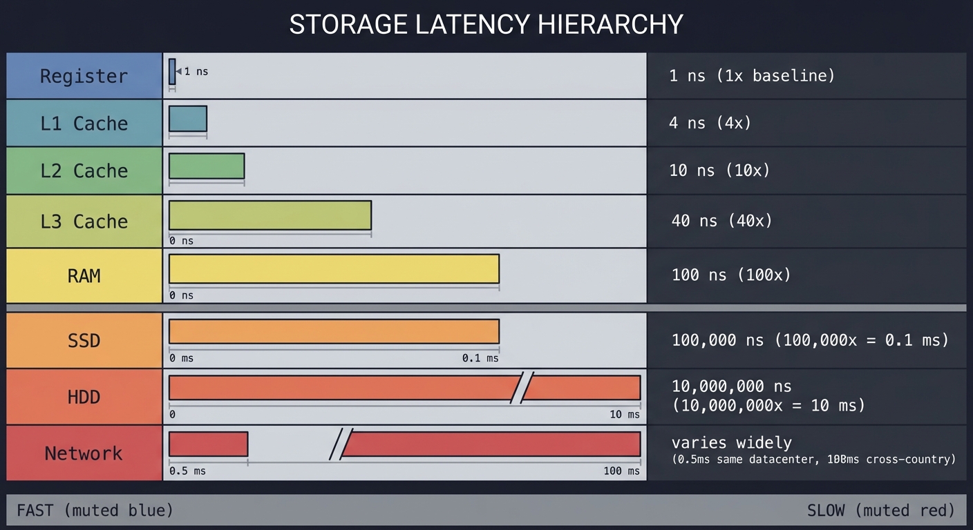
Latency ladder (approximate): Accessing L1 cache is about 0.5 ns, main memory about 100 ns, and disk about 10 ms. That is a difference of roughly 20,000,000x between cache and disk. A single bad data structure choice can push your workload from cache-friendly to memory- or disk-bound.

Source: Jeff Dean latency numbers (2012), https://gist.githubusercontent.com/jboner/2841832/raw/

Memory hierarchy mental model:

CPU registers -> L1 cache -> L2 cache -> L3 cache -> RAM -> SSD -> Disk -> Network
   fast            fast        fast        fast       slower  slower  slower  slowest

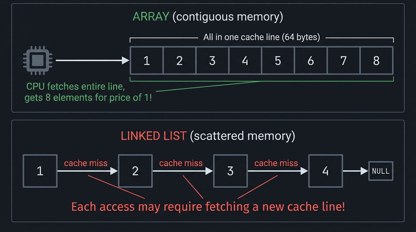
A concrete cache fact: Modern CPUs move data in fixed-size cache lines. A common size is 64 bytes, which means a contiguous array can fetch multiple elements per line, while a linked list often fetches only one useful node per line.

Source: https://en.wikipedia.org/wiki/Cache_line

History in one line: Arrays and linked lists solved early memory layout problems; trees and heaps made search and scheduling fast; hash tables made lookup near-constant; graphs model the connected world.

Practical examples:

• Search box autocomplete: tries, heaps, and arrays for top-k ranking
• Web caches: hash tables + linked lists for O(1) LRU
• Databases: B-trees for range scans, hash indexes for equality lookups
• Schedulers: heaps and queues for fairness and priority

Bottom line: Data structures decide whether your program fits in cache, scales to millions of records, or collapses under load.

Prerequisites & Background Knowledge

Essential Prerequisites (Must Have)

• C basics: structs, pointers, dynamic allocation, arrays
• Big-O notation and basic algorithm analysis
• Comfort reading and writing small C programs
• Ability to trace pointer values in a debugger

Helpful But Not Required

• Basic systems knowledge: stack vs heap memory
• Familiarity with recursion
• Some exposure to CLI tools (make, gcc/clang)
• Basic understanding of CPU caches and memory latency

Self-Assessment Questions

• Can you explain what a pointer is in one sentence?
• Can you write a function that reallocates and copies an array?
• Can you reason about O(n) vs O(log n) for a search operation?
• Can you draw a linked list and show how a delete works?
• Can you explain the difference between stack allocation and heap allocation?

Development Environment Setup

• C compiler: clang or gcc
• Debugging: gdb or lldb
• Memory checks: valgrind (Linux) or leaks (macOS)
• Optional: perf or Instruments for profiling
• Optional: hyperfine for micro-benchmarking

Time Investment

• Projects 1-2: 1 week each
• Projects 3-4: 1 week each
• Projects 5-8: 1-2 weeks each
• Project 9: 4-6 weeks
• Total path: ~12-16 weeks at 5-8 hours/week

Important Reality Check

You will debug memory issues. Expect segfaults, leaks, and off-by-one bugs. This is the real lesson, and it is exactly how you develop engineering intuition.

Core Concept Analysis

1) Invariants Are the Contract

Every data structure lives or dies by an invariant. Examples:

• Dynamic array: data is contiguous, size <= capacity
• Linked list: each node points to the next, and no cycles (unless you choose to)
• BST: left subtree < node < right subtree
• Heap: parent <= children (min-heap)

2) Time Complexity vs Real Performance

Big-O explains growth, but constants and memory locality decide practical speed.

Two O(n) loops can differ by 10x if one is cache-friendly.

Also remember: algorithmic complexity assumes uniform memory access, but real hardware is hierarchical. The same data structure can behave differently when it spills from L1 to L3 or out to RAM.

3) Memory Layout and Cache Locality

Arrays walk memory linearly; linked structures jump around.

Contiguous:  [A][B][C][D] -> 1 cache line fetch gets multiple elements
Scattered:   [A] -> [B] -> [C] -> [D] -> many cache misses

A 64-byte cache line can hold 16 integers (4 bytes each). That means iterating a contiguous array can hit 16 items per line, while a linked list might trigger a miss per node.

4) Amortized Analysis

Some operations are expensive occasionally, but cheap on average. Dynamic array growth is the classic case. Amortized analysis tells you when occasional spikes are acceptable and when they are not (e.g., real-time systems).

5) Ownership and Lifetimes

Every node you allocate must be freed. Every pointer you store must remain valid. This is the hardest part in C and also the most important for reliability.

6) Choosing the Right Structure

Ask: “What is the dominant operation?” and “What is the working set size?”

If the dominant operation is “find by key,” a hash table wins. If it is “iterate in order,” a BST or sorted array wins. If it is “find min,” a heap wins.

Concept Summary Table

Concept	What You Must Internalize	Where It Appears	Failure Mode If Wrong
Contiguous memory	Indexing and cache behavior	Project 1, 7	Cache misses, slow scans
Pointers and ownership	Lifetime and safety	Project 2, 5	Leaks, use-after-free
LIFO vs FIFO	Ordering guarantees	Project 3, 4	Incorrect behavior
Hashing	Uniform distribution and collisions	Project 5	O(n) lookup
Tree ordering	Log-time operations	Project 6	Degenerate linked list
Partial ordering	Priority systems	Project 7	Wrong priority
Graph traversal	Reachability and shortest path	Project 8	Wrong paths
On-disk structures	Paging, B-trees	Project 9	Excessive I/O

Deep Dive Reading by Concept

Concept	Book and Chapter
Arrays, pointers, memory layout	Computer Systems: A Programmer’s Perspective, Ch 2-3
Dynamic arrays, amortized analysis	Introduction to Algorithms (CLRS), Ch 17
Lists, stacks, queues	CLRS, Ch 10
Hashing	CLRS, Ch 11; Algorithms, Fourth Edition, Ch 3.4
Trees and BSTs	CLRS, Ch 12; Algorithms, Fourth Edition, Ch 3.2
Heaps and priority queues	CLRS, Ch 6
Graphs and traversal	CLRS, Ch 22-24
B-trees and storage	CLRS, Ch 18; Database Internals, Ch 1-4
C memory management	C Programming: A Modern Approach, Ch 11-12
Practical C implementations	Mastering Algorithms with C, Ch 1-5

Quick Start (First 48 Hours)

Day 1:

• Implement a bump allocator and a tiny dynamic array.
• Add debug prints that show addresses and capacity growth.
• Track how many copies are done during growth.

Day 2:

• Implement a singly linked list and visualize nodes with addresses.
• Measure iteration time vs dynamic array for 1M elements.
• Write a short README explaining the trade-off you observed.

Recommended Learning Paths

1) Systems Path (C-heavy)

• Projects 1 -> 2 -> 4 -> 5 -> 6 -> 7 -> 9
• Focus: memory layout, performance, correctness under load

2) Interview Path (theory-first)

• Projects 1 -> 2 -> 3 -> 4 -> 5 -> 6 -> 8
• Focus: explaining invariants, common questions, big-O reasoning

3) Product Path (practical impact)

• Projects 1 -> 2 -> 5 -> 7 -> 8 -> 9
• Focus: caching, scheduling, data access, real-world trade-offs

Big Picture / Mental Model

Problem -> Dominant operation -> Candidate structures -> Memory layout -> Performance

Find by key?   -> hash table, BST
Find min/max?  -> heap
Order matters? -> array, BST
Sequence?      -> array, linked list, deque
Relationships? -> graph
Disk data?     -> B-tree, log-structured

Success Metrics

• You can implement array, list, stack, queue, hash table, BST, heap, and graph from scratch.
• You can explain the invariant of each structure without notes.
• You can predict time complexity and typical constant-factor behavior.
• You can debug memory errors with a tool and fix them confidently.
• You can justify a structure choice for a real product scenario.
• You can explain how cache behavior changes the performance story.

How to Use This Guide

1. Read the concept analysis before each project.
2. Build the project and print internal states (addresses, pointers, sizes).
3. Compare real timings with theoretical complexity.
4. Answer the design questions and interview prompts.
5. Use the definition of done to verify completeness.
6. Keep a running log of bugs and fixes; that log is the real learning artifact.

Core System Walkthrough: From Problem to Cache Lines

User problem -> Operations (find, insert, delete) -> Data structure choice
-> Memory layout -> Cache behavior -> Real runtime cost

If you get the structure wrong, the CPU spends time waiting on memory instead of computing.

This is why structures that minimize pointer chasing and maximize contiguous access often win in practice.

Implementation Navigation Cheatsheet

Use consistent file naming so your future self can navigate:

• array.c/.h, list.c/.h, stack.c/.h, queue.c/.h
• hash.c/.h, bst.c/.h, heap.c/.h, graph.c/.h

Useful rg searches when debugging:

• rg "struct .*Node" to find node layouts
• rg "malloc\\(" to audit allocations
• rg "free\\(" to verify cleanup
• rg "size|capacity|count" to find size invariants
• rg "assert\\(" to find invariant checks

Debugging Toolkit

• AddressSanitizer: clang -fsanitize=address -g
• Valgrind: valgrind --leak-check=full ./your_program
• GDB: gdb ./your_program then run, bt, frame
• Perf (Linux): perf stat ./your_program
• hexdump -C to inspect binary structures

Data Structure Atlas (Core Structs and Invariants)

Structure	Core Structs	Invariant
Dynamic Array	data, size, capacity	size <= capacity, contiguous
Linked List	Node{data,next}	next is NULL at tail
Stack	items, top	top == -1 when empty
Queue	front, rear, size	size tracks elements in ring
Hash Table	buckets, Entry{key,value,next}	load factor < threshold
BST	Node{key,left,right}	left < key < right
Heap	data[]	heap property for all nodes
Graph	adj_list[]	each edge recorded consistently

Contribution Checklist (For Your Own Code)

• Each structure has unit tests for empty, single, and many elements.
• All allocations are paired with frees.
• Invariants are checked with debug asserts.
• Benchmarks are repeatable with fixed seeds.
• README explains the trade-offs and use cases.
• Benchmark results include CPU and memory profile notes.

Glossary of Data Structure Terms

• Invariant: A rule that must always hold for correctness.
• Amortized: Average cost over a sequence of operations.
• Load factor: Entries / buckets in a hash table.
• Rotation: Tree operation that preserves ordering but changes shape.
• Sentinel: Special node that simplifies edge cases.
• Adjacency list: Per-node list of edges in a graph.
• Cache line: Fixed-size block of data moved between memory and cache.
• Tombstone: A deleted slot marker in open addressing.
• Balance factor: Height difference between left and right subtrees.
• Topology: The shape of connections in a graph.

Common Failure Signatures

Problem: “Segmentation fault on delete”

• Why: Node pointers not updated correctly.
• Fix: Trace prev/next updates and validate NULL cases.
• Quick test: Delete head, tail, and middle from a 3-node list.

Problem: “Hash table becomes slow”

• Why: Load factor too high or poor hash distribution.
• Fix: Resize earlier and test with adversarial keys.
• Quick test: Insert 1M sequential keys and measure collisions.

Problem: “Heap returns wrong min”

• Why: Heapify swap logic broken or index math off-by-one.
• Fix: Validate parent/child indices and run heap invariant checks.
• Quick test: After every insert, scan array to verify parent <= children.

Problem: “BFS path length is too long”

• Why: Using DFS instead of BFS or not tracking distances.
• Fix: Use a queue and distance array.
• Quick test: Compare BFS distance to a known shortest path.

Problem: “AVL rotations corrupt tree”

• Why: Incorrect child reassignment or height update.
• Fix: Validate rotation logic with 3-node cases.
• Quick test: Insert 3 nodes that trigger each rotation case.

Reading Plan (Daily, Lightweight)

Day 1-2: Arrays, pointers, memory layout (CSAPP Ch 2-3) Day 3-4: Linked lists, stacks, queues (CLRS Ch 10) Day 5-6: Hash tables (CLRS Ch 11) Day 7-9: Trees and balancing (CLRS Ch 12-13) Day 10-12: Heaps and priority queues (CLRS Ch 6) Day 13-16: Graphs (CLRS Ch 22-24) Day 17+: B-trees and database internals (CLRS Ch 18, Database Internals Ch 1-4)

If you only have 30 minutes/day, focus on one structure per week and implement a tiny version with tests.

Part 1: Why Do Data Structures Exist?

The Fundamental Problem

Every program needs to store and organize collections of data. But here’s the critical insight:

How you organize data determines how fast your program runs.

Consider this: You have 1 million user records. How do you store them?

Operation	Unsorted Array	Sorted Array	Hash Table	Binary Search Tree
Find user by ID	O(n) = 1M checks	O(log n) = 20 checks	O(1) = 1 check	O(log n) = 20 checks
Add new user	O(1) = instant	O(n) = 1M shifts	O(1) = instant	O(log n) = 20 steps
Delete user	O(n) = 1M checks	O(n) = 1M shifts	O(1) = instant	O(log n) = 20 steps
List in order	O(n log n) = sort	O(n) = just read	O(n log n) = sort	O(n) = in-order walk

There is no perfect data structure. Every choice is a trade-off between:

• Time (how fast are operations?)
• Space (how much memory?)
• Complexity (how hard to implement correctly?)

Workload questions to ask before choosing:

• Are reads more common than writes?
• Is the access pattern random or sequential?
• Do you need ordered traversal or just lookup?
• Will the data fit in memory or spill to disk?

The Mental Model

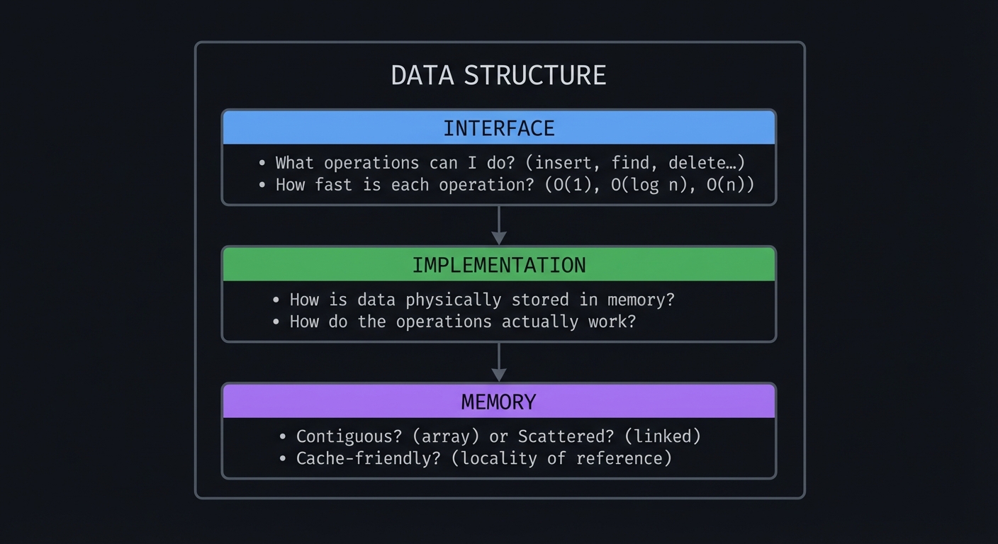
Think of data structures as containers with rules:

┌─────────────────────────────────────────────────────────────────┐
│                    DATA STRUCTURE                                │
│  ┌─────────────────────────────────────────────────────────┐    │
│  │                    INTERFACE                             │    │
│  │  - What operations can I do? (insert, find, delete...)  │    │
│  │  - How fast is each operation? (O(1), O(log n), O(n))   │    │
│  └─────────────────────────────────────────────────────────┘    │
│                              │                                   │
│                              ▼                                   │
│  ┌─────────────────────────────────────────────────────────┐    │
│  │                  IMPLEMENTATION                          │    │
│  │  - How is data physically stored in memory?             │    │
│  │  - How do the operations actually work?                 │    │
│  └─────────────────────────────────────────────────────────┘    │
│                              │                                   │
│                              ▼                                   │
│  ┌─────────────────────────────────────────────────────────┐    │
│  │                    MEMORY                                │    │
│  │  - Contiguous? (array) or Scattered? (linked)          │    │
│  │  - Cache-friendly? (locality of reference)              │    │
│  └─────────────────────────────────────────────────────────┘    │
└─────────────────────────────────────────────────────────────────┘

You can also think of them as an “operation contract”: you are paying with memory and complexity to buy specific performance guarantees.

The Data Structure Family Tree

                           Data Structures
                                 │
            ┌────────────────────┴────────────────────┐
            │                                         │
       Linear                                    Non-Linear
            │                                         │
   ┌────────┼────────┐                    ┌──────────┼──────────┐
   │        │        │                    │          │          │
 Array   Linked    Stack                Tree      Graph      Hash
         List      Queue                  │                   Table
                     │           ┌────────┼────────┐
              ┌──────┴──────┐    │        │        │
              │             │   BST     Heap    Trie
           Priority     Deque    │
            Queue              B-Tree
                              AVL/RB

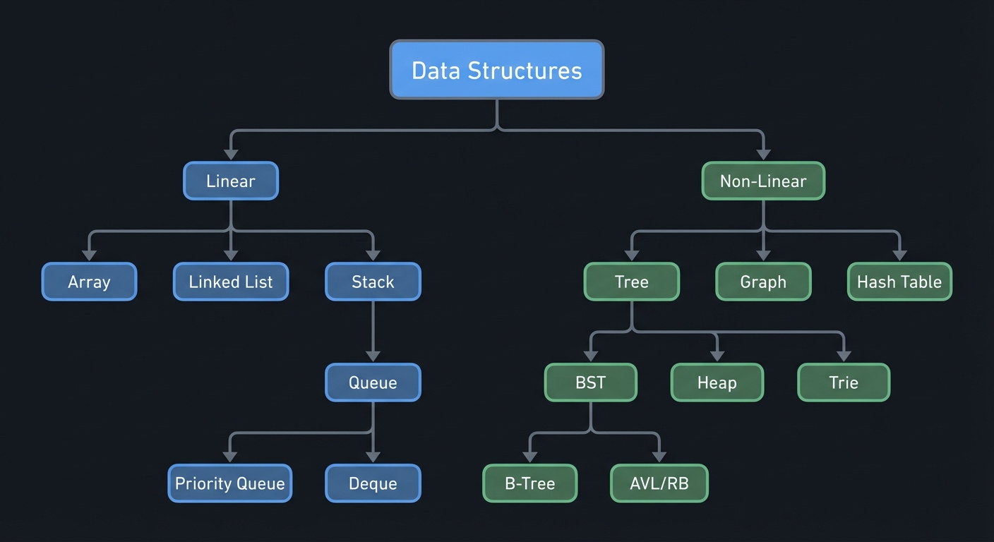
Hybrid structures are common in real systems: LRU = hash table + doubly linked list, priority queues often wrap heaps, and databases blend B-trees, hash tables, and buffer pools.

---

Part 2: The Learning Path

Phase 1: Foundations (3-4 weeks)

1. Project 1: Memory Arena & Dynamic Array
2. Project 2: Linked List Toolkit
   • Outcome: you can reason about raw memory and pointer ownership.

Phase 2: Abstract Data Types (2-3 weeks)

1. Project 3: Stack Machine (Calculator/VM)
2. Project 4: Queue Systems (Task Scheduler)
   • Outcome: you can model ordering constraints (LIFO/FIFO).

Phase 3: Fast Lookup (3-4 weeks)

1. Project 5: Hash Table (Dictionary/Cache)
2. Project 6: Binary Search Tree & Balancing
   • Outcome: you can pick between unordered speed and ordered search.

Phase 4: Specialized Structures (3-4 weeks)

1. Project 7: Heap & Priority Queue
2. Project 8: Graph Algorithms Visualizer
   • Outcome: you can schedule and reason about relationships.

Phase 5: Capstone (4-6 weeks)

1. Project 9: Mini Database Engine
   • Outcome: you can combine structures into a real system.

---

Project Comparison Table

Project	Difficulty	Time	Key Insight	Real-World Use	Core Invariant
Memory Arena & Dynamic Array	⭐⭐	1 week	Memory is just bytes	Every program uses arrays	size <= capacity
Linked List Toolkit	⭐⭐	1 week	Pointers connect scattered memory	Undo systems, playlists	tail->next == NULL
Stack Machine	⭐⭐⭐	1 week	LIFO enables recursion/backtracking	Compilers, calculators	top points to last
Queue Systems	⭐⭐⭐	1 week	FIFO enables fairness/ordering	Job schedulers, BFS	front/rear wrap
Hash Table	⭐⭐⭐⭐	2 weeks	Trade space for O(1) lookup	Databases, caches, dictionaries	load factor bounded
BST & Balancing	⭐⭐⭐⭐	2 weeks	Ordering enables fast search	Databases, file systems	left < node < right
Heap & Priority Queue	⭐⭐⭐	1 week	Partial ordering is cheaper	Schedulers, Dijkstra’s	parent <= children
Graph Visualizer	⭐⭐⭐⭐	2 weeks	Relationships are everywhere	Maps, social networks, AI	edges consistent
Mini Database	⭐⭐⭐⭐⭐	4-6 weeks	Combine everything	Real databases	page + index consistency

---

Project 1: Memory Arena & Dynamic Array

• Main Programming Language: C
• Alternative Programming Languages: Rust, Zig
• Coolness Level: Level 4: Hardcore Tech Flex
• Business Potential: 1. The “Resume Gold”
• Difficulty: Level 2: Intermediate
• Knowledge Area: Memory Management / Low-Level Programming
• Software or Tool: Custom memory allocator
• Main Book: Computer Systems: A Programmer’s Perspective by Bryant & O’Hallaron

What you’ll build

A memory arena (bump allocator) and a dynamic array (like C++’s std::vector or Python’s list) from scratch, visualizing memory layout as you add and remove elements.

Deliverables:

• arena.c/.h with allocate/reset/destroy functions
• dynarray.c/.h with push/pop/get/set and growth logic
• A demo program that prints memory addresses and capacity growth

Why it teaches data structures fundamentals

This is where everything starts. Before you can understand ANY data structure, you must understand:

• What is memory? (just a giant array of bytes)
• What is an address? (index into that array)
• What is allocation? (reserving bytes)
• What is contiguous storage? (elements side-by-side)

Most people use malloc() as a black box. By building your own allocator, you’ll see that memory is just bytes, and data structures are just ways of interpreting those bytes.

You will also see the concrete cost of growing arrays and why amortized analysis matters in practice, not just on paper.

Core challenges you’ll face

• Memory as bytes (everything is just numbers at addresses) → maps to memory model
• Pointer arithmetic (address + offset = new address) → maps to array indexing
• Reallocation (grow array when full) → maps to amortized analysis
• Memory fragmentation (holes in memory) → maps to allocator design
• Cache locality (contiguous = fast) → maps to performance
• Alignment (8/16-byte alignment) → maps to hardware efficiency
• Failure handling (out-of-memory) → maps to robust API design

Key Concepts

Concept	Resource
Memory Layout	Computer Systems: A Programmer’s Perspective Chapter 9 - Bryant & O’Hallaron
Pointer Arithmetic	C Programming: A Modern Approach Chapter 12 - K.N. King
Dynamic Arrays	Introduction to Algorithms Chapter 17.4 (Amortized Analysis) - CLRS
Cache Performance	The Lost Art of Structure Packing - Eric S. Raymond
C Allocators	Effective C, 2nd Edition Chapter 12 - Robert C. Seacord

Difficulty & Time

• Difficulty: Intermediate
• Time estimate: 1 week
• Prerequisites: Basic C, understanding of pointers
• Stretch goal: Add reserve and shrink_to_fit

Real World Outcome

$ ./memory_demo

=== Memory Arena Demo ===
Arena created: 1MB at address 0x7f1234500000

Allocating 100 bytes... got 0x7f1234500000
Allocating 200 bytes... got 0x7f1234500064  (offset: 100)
Allocating 50 bytes...  got 0x7f123450012C  (offset: 300)

Memory map:
[0x7f1234500000] ████████████████████░░░░░░░░░░░░░░░░░░░░░░░░░░░░░░░░
                 ^100 bytes    ^200 bytes  ^50 bytes     ^free space

Arena reset! All allocations freed instantly (no individual free calls needed)

=== Dynamic Array Demo ===
Creating dynamic array with initial capacity 4...

Push 1: [1, _, _, _]           capacity=4, size=1
Push 2: [1, 2, _, _]           capacity=4, size=2
Push 3: [1, 2, 3, _]           capacity=4, size=3
Push 4: [1, 2, 3, 4]           capacity=4, size=4
Push 5: [1, 2, 3, 4, 5, _, _, _]  capacity=8, size=5  ← GREW! (copied to new memory)

Memory addresses:
  Before grow: data at 0x7f1234600000
  After grow:  data at 0x7f1234700000 (new location!)

Performance test: push 1,000,000 elements
  Total time: 0.023s
  Total reallocations: 20 (log2 of 1M)
  Amortized cost per push: O(1) ✓

Random access test:
  arr[0] = 1       (0.000001ms)
  arr[500000] = ?  (0.000001ms)  ← Same speed! O(1) random access ✓

You should be able to explain why the final capacity is a power of two and why the data pointer changes after a resize.

The Core Question You’re Answering

How can I grow a contiguous array without losing data, while keeping average inserts fast and memory overhead predictable? And how do I expose this to callers without leaking memory or breaking invariants?

Concepts You Must Understand First

• Pointer arithmetic and array indexing (C Programming: A Modern Approach, Ch 12)
• Dynamic allocation and reallocation (C Programming: A Modern Approach, Ch 17)
• Amortized analysis (CLRS, Ch 17)
• Alignment and padding (Computer Systems: A Programmer’s Perspective, Ch 2)
• Cache lines and locality (see cache line source above)

Questions to Guide Your Design

• What growth factor keeps reallocation rare without wasting too much memory?
• How do you represent size vs capacity so invariants are explicit?
• What should happen when allocation fails (return NULL, abort, or recover)?
• How will you visualize memory so bugs become obvious?
• Should your API allow random inserts, or is push/pop enough for now?

Thinking Exercise

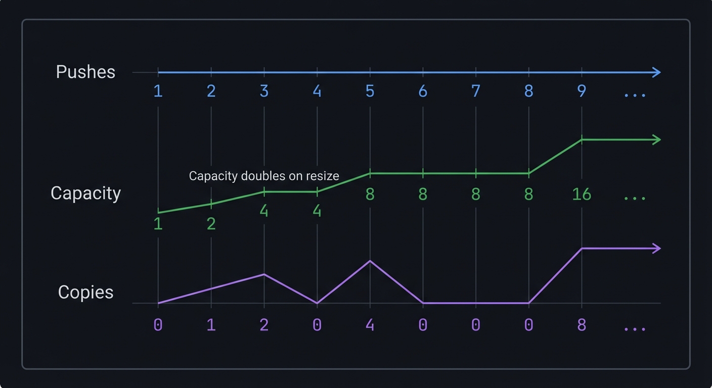
Simulate pushes into a dynamic array starting at capacity 1. For 10 inserts, write down the capacity after each push and count how many total copies occur. Then repeat with a growth factor of 1.5 and compare total copies.

The Interview Questions They’ll Ask

• Why is push_back amortized O(1) but insert in the middle O(n)?
• When do pointer or reference invalidation problems occur in vectors?
• What is the difference between malloc, calloc, and realloc?
• How does alignment affect performance on modern CPUs?
• Why is contiguous memory more cache-friendly?
• How does a ring buffer differ from a dynamic array?

Hints in Layers

1) Start with a bump allocator that never frees. It is just a base pointer and an offset. 2) For the dynamic array, store data, size, and capacity in a struct. 3) Grow only when size == capacity, then allocate new memory and copy. 4) Validate with a tiny example first, then scale. 5) Track the number of copies to verify amortized behavior.

if (arr->size == arr->capacity) {
    size_t new_cap = arr->capacity ? arr->capacity * 2 : 4;
    int* new_data = malloc(new_cap * sizeof(int));
    memcpy(new_data, arr->data, arr->size * sizeof(int));
    free(arr->data);
    arr->data = new_data;
    arr->capacity = new_cap;
}

Books That Will Help

Topic	Book	Why It Helps
Memory layout	Computer Systems: A Programmer’s Perspective, Ch 2-3	Explains how memory is addressed
Pointers	C Programming: A Modern Approach, Ch 11-12	Concrete pointer mechanics
Amortized analysis	CLRS, Ch 17	Formal reasoning for growth strategy
Allocators	C Interfaces and Implementations, Ch 2	Real allocator patterns

Common Pitfalls & Debugging

Problem: “Segfault during array growth”

• Why: realloc or malloc failed or copy used wrong size.
• Fix: Check for NULL, copy size * sizeof(T), not capacity.
• Quick test: Push 1..1000 and verify all values.

Problem: “Arena returns overlapping blocks”

• Why: Alignment or offset update is wrong.
• Fix: Align size and update offset after returning pointer.
• Quick test: Allocate three blocks and assert addresses increase.

Problem: “Memory leak after resize”

• Why: Old buffer not freed after copy.
• Fix: Free the old pointer after successful copy.
• Quick test: Run with ASan or Valgrind.

Problem: “Capacity never grows”

• Why: size not incremented or growth check uses wrong comparison.
• Fix: Increment size on successful push and check size >= capacity.
• Quick test: Push until over initial capacity and verify growth.

Definition of Done

• Arena can allocate multiple blocks and reset in O(1)
• Dynamic array grows correctly and preserves all values
• Invariants (size <= capacity) enforced with asserts
• Benchmarks show amortized O(1) push behavior
• Memory checks report zero leaks
• Growth factor and trade-offs documented in README

Learning Milestones

1. Arena allocates bytes → You understand memory is just bytes
2. Dynamic array grows → You understand reallocation and copying
3. Growth is O(1) amortized → You understand why doubling works
4. Random access is O(1) → You understand contiguous memory
5. Memory layout is visible → You can reason about cache behavior

Implementation

Memory Arena (Bump Allocator)

#include <stdio.h>
#include <stdlib.h>
#include <stdint.h>
#include <string.h>

typedef struct {
    uint8_t* base;      // Start of memory block
    size_t size;        // Total size
    size_t offset;      // Current position (bump pointer)
} Arena;

Arena* arena_create(size_t size) {
    Arena* arena = malloc(sizeof(Arena));
    arena->base = malloc(size);
    arena->size = size;
    arena->offset = 0;
    printf("Arena created: %zu bytes at %p\n", size, arena->base);
    return arena;
}

void* arena_alloc(Arena* arena, size_t size) {
    // Align to 8 bytes for performance
    size_t aligned_size = (size + 7) & ~7;

    if (arena->offset + aligned_size > arena->size) {
        printf("Arena out of memory!\n");
        return NULL;
    }

    void* ptr = arena->base + arena->offset;
    arena->offset += aligned_size;

    printf("Allocated %zu bytes at %p (offset: %zu)\n",
           size, ptr, arena->offset - aligned_size);
    return ptr;
}

void arena_reset(Arena* arena) {
    arena->offset = 0;  // Instant "free" of everything!
    printf("Arena reset! All memory available again.\n");
}

void arena_destroy(Arena* arena) {
    free(arena->base);
    free(arena);
}

// Visualize memory usage
void arena_visualize(Arena* arena) {
    printf("\nMemory map (%zu / %zu bytes used):\n[", arena->offset, arena->size);
    int blocks = 50;
    int used = (arena->offset * blocks) / arena->size;
    for (int i = 0; i < blocks; i++) {
        printf("%s", i < used ? "█" : "░");
    }
    printf("]\n\n");
}

Dynamic Array

typedef struct {
    int* data;          // Pointer to array
    size_t size;        // Number of elements
    size_t capacity;    // Allocated space
} DynArray;

DynArray* dynarray_create(size_t initial_capacity) {
    DynArray* arr = malloc(sizeof(DynArray));
    arr->data = malloc(initial_capacity * sizeof(int));
    arr->size = 0;
    arr->capacity = initial_capacity;
    printf("Created array with capacity %zu at %p\n",
           initial_capacity, arr->data);
    return arr;
}

void dynarray_push(DynArray* arr, int value) {
    // Check if we need to grow
    if (arr->size >= arr->capacity) {
        size_t new_capacity = arr->capacity * 2;  // Double!
        int* new_data = malloc(new_capacity * sizeof(int));

        // Copy old data to new location
        memcpy(new_data, arr->data, arr->size * sizeof(int));

        printf("GROW: %zu -> %zu (moved from %p to %p)\n",
               arr->capacity, new_capacity, arr->data, new_data);

        free(arr->data);
        arr->data = new_data;
        arr->capacity = new_capacity;
    }

    arr->data[arr->size++] = value;
}

int dynarray_get(DynArray* arr, size_t index) {
    if (index >= arr->size) {
        printf("Index out of bounds!\n");
        return -1;
    }
    return arr->data[index];  // O(1) - just pointer + offset!
}

void dynarray_visualize(DynArray* arr) {
    printf("[");
    for (size_t i = 0; i < arr->capacity; i++) {
        if (i < arr->size) {
            printf("%d", arr->data[i]);
        } else {
            printf("_");
        }
        if (i < arr->capacity - 1) printf(", ");
    }
    printf("]  size=%zu, capacity=%zu\n", arr->size, arr->capacity);
}

Design Notes

• Keep size and capacity in the same struct to make invariants explicit.
• Use a growth factor (2x is simplest; 1.5x is more memory efficient).
• Always check allocation results and keep the old pointer until new memory is confirmed.
• Consider alignment if you plan to store structs with stricter alignment than int.

Testing & Validation

• Push 1..N, then verify arr[i] == i+1 for all i.
• Force multiple resizes by starting at capacity 1 and pushing 1,000+ items.
• Use ASan/Valgrind to confirm no leaks or invalid accesses.

Performance Experiments

• Compare iteration time between dynamic array and linked list for 1M elements.
• Track number of reallocations and total bytes copied during growth.
• Plot time per push as array grows to visualize amortization.

Dynamic Array Growth Timeline (capacity doubles)

Pushes:   1 2 3 4 5 6 7 8 9 ...
Capacity: 1 2 4 4 8 8 8 8 16 ...
Copies:   0 1 2 0 4 0 0 0 8 ...

Why Arrays Are Cache-Friendly

ARRAY (contiguous memory):
┌───┬───┬───┬───┬───┬───┬───┬───┐
│ 1 │ 2 │ 3 │ 4 │ 5 │ 6 │ 7 │ 8 │  ← All in one cache line (64 bytes)
└───┴───┴───┴───┴───┴───┴───┴───┘
  ↑
  CPU fetches entire line, gets 8 elements for price of 1!

LINKED LIST (scattered memory):
┌───┐     ┌───┐     ┌───┐     ┌───┐
│ 1 │────►│ 2 │────►│ 3 │────►│ 4 │
└───┘     └───┘     └───┘     └───┘
  ↑ cache miss  ↑ cache miss  ↑ cache miss
  Each access may require fetching a new cache line!

The Amortization Insight

Why does doubling capacity give O(1) amortized push?

Operations to push n elements:
  n pushes (always)
  + copy 1 element (when growing from 1 to 2)
  + copy 2 elements (when growing from 2 to 4)
  + copy 4 elements (when growing from 4 to 8)
  + ...
  + copy n/2 elements (when growing from n/2 to n)

Total copies = 1 + 2 + 4 + ... + n/2 = n - 1

Total work = n pushes + (n-1) copies ≈ 2n = O(n)
Average work per push = O(n) / n = O(1) ✓

---

Project 2: Linked List Toolkit

• Main Programming Language: C
• Alternative Programming Languages: Rust, Go, Python
• Coolness Level: Level 3: Genuinely Clever
• Business Potential: 1. The “Resume Gold”
• Difficulty: Level 2: Intermediate
• Knowledge Area: Pointers / Dynamic Memory
• Software or Tool: CLI list manipulation tool
• Main Book: C Programming: A Modern Approach by K.N. King

What you’ll build

A comprehensive linked list library (singly-linked, doubly-linked, circular) with visualization, plus a practical application: an undo/redo system for a text editor.

Deliverables:

• sll.c/.h, dll.c/.h, cll.c/.h with insert/delete/search
• A list visualizer that prints node addresses and links
• Undo/redo demo with stack semantics

Why it teaches this concept

Linked lists are the opposite of arrays:

• Arrays: contiguous memory, random access, expensive insert/delete
• Linked lists: scattered memory, sequential access, cheap insert/delete

Understanding this trade-off is fundamental. You’ll also master pointers, which are essential for all complex data structures.

You also see why pointer-heavy structures often lose to arrays for iteration-heavy workloads despite better asymptotic insertion behavior.

Core challenges you’ll face

• Pointer manipulation (next, prev, head, tail) → maps to indirection
• Edge cases (empty list, one element, head/tail operations) → maps to boundary conditions
• Memory management (malloc each node, free on remove) → maps to manual memory
• Traversal (must walk from head) → maps to O(n) access
• Doubly-linked (can go backwards) → maps to trade-offs
• Sentinel nodes (optional) → maps to simplifying edge cases

Key Concepts

Concept	Resource
Pointer Fundamentals	C Programming: A Modern Approach Chapter 11 - K.N. King
Linked List Operations	Introduction to Algorithms Chapter 10.2 - CLRS
Memory Allocation	The C Programming Language Chapter 7 - K&R
Data Structures in C	Mastering Algorithms with C Chapter 3-4 - Kyle Loudon

Difficulty & Time

• Difficulty: Intermediate
• Time estimate: 1 week
• Prerequisites: Project 1 completed, comfortable with pointers
• Stretch goal: Add a list iterator API

Real World Outcome

$ ./linkedlist_demo

=== Singly Linked List ===
Insert 10 at head: [10] -> NULL
Insert 20 at head: [20] -> [10] -> NULL
Insert 30 at tail: [20] -> [10] -> [30] -> NULL
Insert 25 after 10: [20] -> [10] -> [25] -> [30] -> NULL

Memory layout:
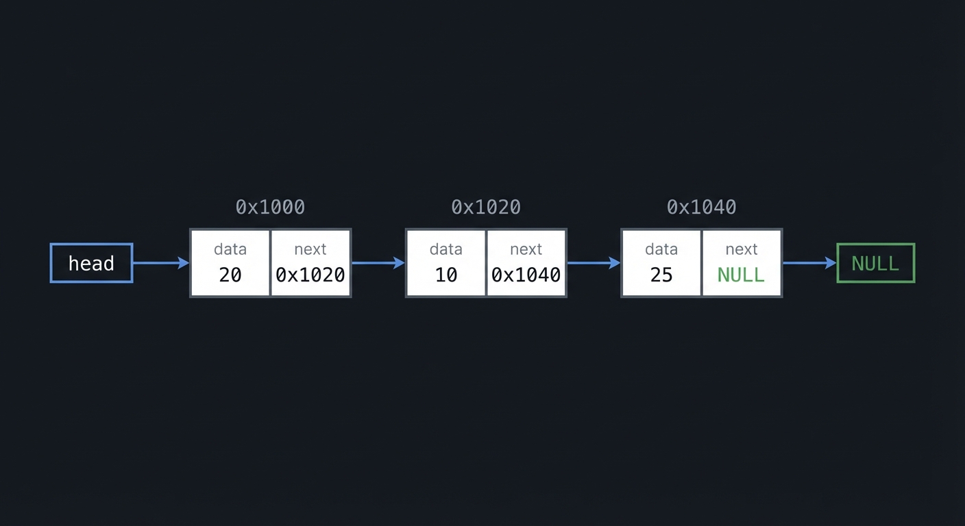
  Node@0x1000: data=20, next=0x1020
  Node@0x1020: data=10, next=0x1040
  Node@0x1040: data=25, next=0x1060
  Node@0x1060: data=30, next=NULL

Delete 10: [20] -> [25] -> [30] -> NULL
  (freed memory at 0x1020)

=== Doubly Linked List ===
[NULL <-> 20 <-> 25 <-> 30 <-> NULL]
Traverse forward:  20 -> 25 -> 30
Traverse backward: 30 -> 25 -> 20

=== Undo/Redo System Demo ===
Text: ""
> type "Hello"
Text: "Hello"                    [undo stack: "Hello"]
> type " World"
Text: "Hello World"              [undo stack: "Hello", " World"]
> undo
Text: "Hello"                    [redo stack: " World"]
> undo
Text: ""                         [redo stack: " World", "Hello"]
> redo
Text: "Hello"                    [undo stack: "Hello"]
> type "!"
Text: "Hello!"                   [redo stack cleared!]

You should be able to point to any node address and explain which pointers connect to it and why.

The Core Question You’re Answering

When data is scattered across memory, how do I connect it safely and still support fast insert and delete operations? And how do I prevent pointer bugs when the structure changes frequently?

Concepts You Must Understand First

• Pointer ownership and lifetime (C Programming: A Modern Approach, Ch 11-12)
• Dynamic allocation and freeing (C Programming: A Modern Approach, Ch 17)
• Linked list operations (CLRS, Ch 10.2)
• Big-O trade-offs for sequential access (Algorithms, Fourth Edition, Ch 1.3)
• Sentinel nodes and edge cases (Mastering Algorithms with C, Ch 3)

Questions to Guide Your Design

• What invariants make a list correct (head, tail, NULL termination)?
• How do you delete a node when you do not have a pointer to the previous node?
• When should you use a sentinel node to simplify edge cases?
• How will you prevent memory leaks in undo/redo stacks?
• How will you handle duplicate values or stable ordering?

Thinking Exercise

Draw a 3-node doubly linked list and simulate deleting the middle node. Write down which pointers change in what order. Then simulate deleting the head and tail.

The Interview Questions They’ll Ask

• Why is random access O(n) in a linked list?
• What is the difference between singly and doubly linked lists?
• How do you detect a cycle in a linked list?
• When is a linked list better than a dynamic array?
• How do you implement an LRU cache with a linked list?
• What is the memory overhead per node?

Hints in Layers

1) Start with a simple singly linked list with head and tail. 2) Add a size field to make correctness checks easy. 3) Move to a doubly linked list and implement delete-with-node-pointer. 4) Build undo/redo stacks on top of the list or stack abstraction. 5) Add a list_validate() function that checks invariants.

// Delete node in doubly linked list when you have the node pointer.
if (node->prev) node->prev->next = node->next;
else list->head = node->next;
if (node->next) node->next->prev = node->prev;
else list->tail = node->prev;
free(node);

Books That Will Help

Topic	Book	Why It Helps
Linked lists	CLRS, Ch 10.2	Formal list operations
Pointers	C Programming: A Modern Approach, Ch 11	Pointer manipulation
Memory management	The C Programming Language, Ch 7	Allocation and freeing
Practical list APIs	Mastering Algorithms with C, Ch 3	C-focused patterns

Common Pitfalls & Debugging

Problem: “List prints garbage after delete”

• Why: Forgot to update next or prev on neighbors.
• Fix: Update neighbors first, then free.
• Quick test: Delete head, tail, and middle in a 3-node list.

Problem: “Infinite loop during traversal”

• Why: Created a cycle unintentionally.
• Fix: Ensure tail->next is NULL and update pointers carefully.
• Quick test: Detect cycle with fast/slow pointers.

Problem: “Undo history leaks memory”

• Why: Actions not freed when cleared.
• Fix: Walk the stack and free each node and payload.
• Quick test: Use Valgrind after a long undo/redo session.

Problem: “Tail pointer is wrong”

• Why: Tail not updated on delete or insert at end.
• Fix: Update tail on head/tail operations.
• Quick test: Append 3 nodes, delete tail, and check tail address.

Definition of Done

• Singly, doubly, and circular lists pass unit tests
• All edge cases (empty, single, head/tail) handled
• Undo/redo behavior matches expected stack semantics
• No memory leaks under stress tests
• Runtime trade-offs documented in README
• Cycle detection test added (Floyd’s algorithm)

Learning Milestones

1. Insert/delete at head is O(1) → You understand the advantage over arrays
2. Find element is O(n) → You understand the disadvantage
3. Doubly-linked enables O(1) delete given node → You understand the trade-off
4. Undo/redo works → You understand why linked lists exist in real systems
5. Memory cleanup is correct → You understand ownership and lifetimes

Implementation

Singly Linked List

typedef struct Node {
    int data;
    struct Node* next;
} Node;

typedef struct {
    Node* head;
    Node* tail;
    size_t size;
} SinglyLinkedList;

// O(1) - just update head
void sll_push_front(SinglyLinkedList* list, int data) {
    Node* new_node = malloc(sizeof(Node));
    new_node->data = data;
    new_node->next = list->head;

    list->head = new_node;
    if (list->tail == NULL) {
        list->tail = new_node;
    }
    list->size++;
}

// O(1) - just update tail
void sll_push_back(SinglyLinkedList* list, int data) {
    Node* new_node = malloc(sizeof(Node));
    new_node->data = data;
    new_node->next = NULL;

    if (list->tail) {
        list->tail->next = new_node;
    } else {
        list->head = new_node;
    }
    list->tail = new_node;
    list->size++;
}

// O(n) - must traverse to find
Node* sll_find(SinglyLinkedList* list, int data) {
    Node* current = list->head;
    while (current) {
        if (current->data == data) {
            return current;
        }
        current = current->next;
    }
    return NULL;
}

// O(n) - must find previous node
void sll_delete(SinglyLinkedList* list, int data) {
    if (!list->head) return;

    // Special case: deleting head
    if (list->head->data == data) {
        Node* to_delete = list->head;
        list->head = list->head->next;
        if (list->tail == to_delete) {
            list->tail = NULL;
        }
        free(to_delete);
        list->size--;
        return;
    }

    // Find previous node
    Node* prev = list->head;
    while (prev->next && prev->next->data != data) {
        prev = prev->next;
    }

    if (prev->next) {
        Node* to_delete = prev->next;
        prev->next = to_delete->next;
        if (list->tail == to_delete) {
            list->tail = prev;
        }
        free(to_delete);
        list->size--;
    }
}

void sll_print(SinglyLinkedList* list) {
    Node* current = list->head;
    while (current) {
        printf("[%d]", current->data);
        if (current->next) printf(" -> ");
        current = current->next;
    }
    printf(" -> NULL\n");
}

Doubly Linked List

typedef struct DNode {
    int data;
    struct DNode* prev;
    struct DNode* next;
} DNode;

typedef struct {
    DNode* head;
    DNode* tail;
    size_t size;
} DoublyLinkedList;

// O(1) delete when you have the node pointer!
void dll_delete_node(DoublyLinkedList* list, DNode* node) {
    if (node->prev) {
        node->prev->next = node->next;
    } else {
        list->head = node->next;
    }

    if (node->next) {
        node->next->prev = node->prev;
    } else {
        list->tail = node->prev;
    }

    free(node);
    list->size--;
}

Undo/Redo System (Practical Application)

typedef struct Action {
    char* text;              // The text that was added
    struct Action* next;
} Action;

typedef struct {
    char buffer[1024];       // Current text
    Action* undo_stack;      // Stack of actions to undo
    Action* redo_stack;      // Stack of actions to redo
} TextEditor;

void editor_type(TextEditor* editor, const char* text) {
    // Add to buffer
    strcat(editor->buffer, text);

    // Push to undo stack
    Action* action = malloc(sizeof(Action));
    action->text = strdup(text);
    action->next = editor->undo_stack;
    editor->undo_stack = action;

    // Clear redo stack (can't redo after new action)
    while (editor->redo_stack) {
        Action* to_free = editor->redo_stack;
        editor->redo_stack = editor->redo_stack->next;
        free(to_free->text);
        free(to_free);
    }
}

void editor_undo(TextEditor* editor) {
    if (!editor->undo_stack) {
        printf("Nothing to undo!\n");
        return;
    }

    // Pop from undo stack
    Action* action = editor->undo_stack;
    editor->undo_stack = action->next;

    // Remove text from buffer
    size_t len = strlen(action->text);
    editor->buffer[strlen(editor->buffer) - len] = '\0';

    // Push to redo stack
    action->next = editor->redo_stack;
    editor->redo_stack = action;
}

void editor_redo(TextEditor* editor) {
    if (!editor->redo_stack) {
        printf("Nothing to redo!\n");
        return;
    }

    // Pop from redo stack
    Action* action = editor->redo_stack;
    editor->redo_stack = action->next;

    // Add text back to buffer
    strcat(editor->buffer, action->text);

    // Push to undo stack
    action->next = editor->undo_stack;
    editor->undo_stack = action;
}

Design Notes

• Store head, tail, and size to simplify invariants and reduce traversal.
• Use sentinel nodes if you want to simplify edge-case handling.
• Always update neighbors before freeing a node.
• Separate list logic from application logic (undo/redo) for clarity.

Testing & Validation

• Insert/delete head, tail, and middle nodes in lists of size 0, 1, and 3.
• Run a cycle-detection test (Floyd’s algorithm) after operations.
• Use Valgrind to confirm every node is freed.

Performance Experiments

• Compare delete-at-head vs delete-at-tail timing.
• Measure traversal time vs dynamic array for 1M elements.
• Track memory overhead per node (data + pointers).

Linked List Pointer Layout (singly linked)

head
 |
 v
[0x1000 | data=20 | next=0x1020] -> [0x1020 | data=10 | next=0x1040] -> NULL

Array vs Linked List: The Trade-off

Operation	Array	Linked List	Winner
Access by index	O(1)	O(n)	Array
Insert at beginning	O(n)	O(1)	Linked List
Insert at end	O(1) amortized	O(1) with tail	Tie
Insert in middle	O(n)	O(1) if have node	Linked List
Delete	O(n)	O(1) if have node	Linked List
Memory overhead	Low	High (pointers)	Array
Cache performance	Excellent	Poor	Array

When to use Linked Lists:

• Frequent insertions/deletions at arbitrary positions
• When you have pointers to nodes (e.g., LRU cache)
• When you need O(1) worst-case insert (not amortized)

When to use Arrays:

• Need random access
• Iterating through all elements (cache-friendly)
• Memory is tight (no pointer overhead)

---

Project 3: Stack Machine (Calculator & Mini VM)

• Main Programming Language: C
• Alternative Programming Languages: Rust, Go, Python
• Coolness Level: Level 4: Hardcore Tech Flex
• Business Potential: 1. The “Resume Gold”
• Difficulty: Level 3: Advanced
• Knowledge Area: Abstract Data Types / Language Implementation
• Software or Tool: RPN Calculator, Bytecode VM
• Main Book: Writing a C Compiler by Nora Sandler

What you’ll build

A Reverse Polish Notation (RPN) calculator and a simple stack-based virtual machine that executes bytecode—demonstrating why stacks are fundamental to computing.

Deliverables:

• stack.c/.h with push/pop/peek
• rpn.c evaluator with tokenization
• vm.c with a small bytecode instruction set

Why it teaches this concept

The stack is not just a data structure—it’s how computers work:

• Function calls use a stack (call stack)
• Expression evaluation uses a stack
• Undo operations use a stack
• Backtracking algorithms use a stack
• Your CPU has a hardware stack

Building a stack machine shows you why LIFO (Last In, First Out) is so fundamental.

You also learn to separate parsing from execution, which is core to compilers and interpreters.

Core challenges you’ll face

• LIFO semantics (last in, first out) → maps to stack discipline
• Expression parsing (infix to postfix) → maps to operator precedence
• VM execution (fetch-decode-execute) → maps to computation model
• Stack underflow/overflow → maps to error handling
• Tokenization (numbers and operators) → maps to parsing

Key Concepts

Concept	Resource
Stack ADT	Introduction to Algorithms Chapter 10.1 - CLRS
Expression Evaluation	Algorithms, Fourth Edition Chapter 1.3 - Sedgewick
Stack Machines	Writing a C Compiler Chapter 3 - Nora Sandler
Shunting Yard Algorithm	Dijkstra’s original paper or Wikipedia
Call Stack	Computer Systems: A Programmer’s Perspective Chapter 3

Difficulty & Time

• Difficulty: Intermediate-Advanced
• Time estimate: 1 week
• Prerequisites: Projects 1-2 completed
• Stretch goal: Add variables and a tiny memory model

Real World Outcome

$ ./rpn_calc
RPN Calculator (type 'quit' to exit)

> 3 4 +
Stack: [7]
Result: 7

> 5 *
Stack: [35]
Result: 35

> 2 3 4 + *
Stack: [35, 14]
  Explanation: 2 * (3 + 4) = 14
Result: 14

> clear
Stack: []

=== Infix to RPN Demo ===
Infix:   (3 + 4) * 5
Postfix: 3 4 + 5 *
Result:  35

=== Mini VM Demo ===
Bytecode: PUSH 10, PUSH 20, ADD, PUSH 5, MUL, PRINT
Executing...
  PUSH 10    Stack: [10]
  PUSH 20    Stack: [10, 20]
  ADD        Stack: [30]
  PUSH 5     Stack: [30, 5]
  MUL        Stack: [150]
  PRINT      Output: 150

You should be able to trace the exact stack contents at every step.

The Core Question You’re Answering

How does a stack enable expression evaluation and program execution, and why does LIFO make computation simple? How does this relate to the real CPU call stack?

Concepts You Must Understand First

• Stack ADT operations (CLRS, Ch 10.1)
• Operator precedence and associativity (Algorithms, Fourth Edition, Ch 1.3)
• Tokenization and parsing (Writing a C Compiler, Ch 3)
• Error handling (underflow/overflow)
• Call stack frames and function calls (CSAPP, Ch 3)

Questions to Guide Your Design

• What is the minimal instruction set for a stack VM?
• How will you represent tokens and opcodes?
• How will you report errors without crashing?
• How do you show the stack state after each step?
• How will you handle negative numbers and multi-digit tokens?

Thinking Exercise

Convert (8 - 3) * (2 + 5) to RPN by hand, then evaluate it using a stack trace. Compare the trace to a standard infix evaluation.

The Interview Questions They’ll Ask

• Why is a stack good for parsing expressions?
• What is the difference between a call stack and a data stack?
• How would you implement recursion without a call stack?
• What are common stack overflow conditions?
• How do you parse infix expressions efficiently?
• Why do many bytecode VMs use a stack instead of registers?

Hints in Layers

1) Build a fixed-size stack first, then consider a dynamic version. 2) Implement RPN evaluation with a simple token loop. 3) Add shunting-yard for infix to postfix conversion. 4) Extend to a bytecode VM with opcodes like PUSH, ADD, MUL. 5) Add DUP and SWAP opcodes to experiment with stack manipulation.

if (is_number(token)) stack_push(&s, atoi(token));
else {
    int b = stack_pop(&s);
    int a = stack_pop(&s);
    stack_push(&s, apply_op(token[0], a, b));
}

Books That Will Help

Topic	Book	Why It Helps
Stack operations	CLRS, Ch 10.1	Core ADT behavior
Expression parsing	Algorithms, Fourth Edition, Ch 1.3	Shunting-yard and stacks
VM design	Writing a C Compiler, Ch 3	Stack machines
Call stack	Computer Systems: A Programmer’s Perspective, Ch 3	How functions work

Common Pitfalls & Debugging

Problem: “Stack underflow on operator”

• Why: Missing operands or tokenization error.
• Fix: Validate token stream and check stack size before pop.
• Quick test: Evaluate 3 + and confirm clean error.

Problem: “Wrong precedence”

• Why: Shunting-yard precedence table incorrect.
• Fix: Implement a clear precedence function and unit test.
• Quick test: Compare 3 + 4 * 5 vs (3 + 4) * 5.

Problem: “VM executes garbage”

• Why: Instruction pointer or opcode mapping wrong.
• Fix: Print each instruction and stack state.
• Quick test: Run a 3-instruction program and verify output.

Problem: “Tokenizer merges numbers”

• Why: Missing whitespace handling or digit parsing.
• Fix: Use strtok or a hand-written scanner.
• Quick test: Evaluate 12 3 + and confirm result is 15.

Definition of Done

• RPN evaluator produces correct results for test cases
• Infix to postfix conversion matches known outputs
• VM can execute a small bytecode program end-to-end
• Error handling covers underflow/overflow and bad tokens
• Stack state prints after each step for visibility
• Additional opcodes (DUP, SWAP) are tested

Learning Milestones

1. RPN calculator works → You understand postfix evaluation
2. Infix to postfix conversion works → You understand the shunting-yard algorithm
3. VM executes bytecode → You understand stack machines
4. You see the call stack in action → You understand how functions work
5. Errors are handled gracefully → You understand robust execution

Implementation

Stack Data Structure

#define STACK_MAX 256

typedef struct {
    int items[STACK_MAX];
    int top;
} Stack;

void stack_init(Stack* s) {
    s->top = -1;
}

int stack_is_empty(Stack* s) {
    return s->top == -1;
}

int stack_is_full(Stack* s) {
    return s->top == STACK_MAX - 1;
}

void stack_push(Stack* s, int value) {
    if (stack_is_full(s)) {
        printf("Stack overflow!\n");
        exit(1);
    }
    s->items[++s->top] = value;
}

int stack_pop(Stack* s) {
    if (stack_is_empty(s)) {
        printf("Stack underflow!\n");
        exit(1);
    }
    return s->items[s->top--];
}

int stack_peek(Stack* s) {
    if (stack_is_empty(s)) {
        printf("Stack empty!\n");
        exit(1);
    }
    return s->items[s->top];
}

void stack_print(Stack* s) {
    printf("Stack: [");
    for (int i = 0; i <= s->top; i++) {
        printf("%d", s->items[i]);
        if (i < s->top) printf(", ");
    }
    printf("]\n");
}

RPN Calculator

int evaluate_rpn(const char* expression) {
    Stack stack;
    stack_init(&stack);

    char* expr = strdup(expression);
    char* token = strtok(expr, " ");

    while (token != NULL) {
        if (isdigit(token[0]) || (token[0] == '-' && isdigit(token[1]))) {
            // It's a number - push it
            stack_push(&stack, atoi(token));
        } else {
            // It's an operator - pop operands and compute
            int b = stack_pop(&stack);
            int a = stack_pop(&stack);
            int result;

            switch (token[0]) {
                case '+': result = a + b; break;
                case '-': result = a - b; break;
                case '*': result = a * b; break;
                case '/': result = a / b; break;
                default:
                    printf("Unknown operator: %s\n", token);
                    exit(1);
            }

            stack_push(&stack, result);
        }

        printf("  Token: %-4s  ", token);
        stack_print(&stack);

        token = strtok(NULL, " ");
    }

    free(expr);
    return stack_pop(&stack);
}

Shunting-Yard Algorithm (Infix to Postfix)

int precedence(char op) {
    switch (op) {
        case '+': case '-': return 1;
        case '*': case '/': return 2;
        default: return 0;
    }
}

void infix_to_postfix(const char* infix, char* postfix) {
    Stack op_stack;
    stack_init(&op_stack);

    int j = 0;
    for (int i = 0; infix[i]; i++) {
        char c = infix[i];

        if (isdigit(c)) {
            postfix[j++] = c;
            postfix[j++] = ' ';
        } else if (c == '(') {
            stack_push(&op_stack, c);
        } else if (c == ')') {
            while (!stack_is_empty(&op_stack) && stack_peek(&op_stack) != '(') {
                postfix[j++] = stack_pop(&op_stack);
                postfix[j++] = ' ';
            }
            stack_pop(&op_stack);  // Remove '('
        } else if (c == '+' || c == '-' || c == '*' || c == '/') {
            while (!stack_is_empty(&op_stack) &&
                   precedence(stack_peek(&op_stack)) >= precedence(c)) {
                postfix[j++] = stack_pop(&op_stack);
                postfix[j++] = ' ';
            }
            stack_push(&op_stack, c);
        }
    }

    while (!stack_is_empty(&op_stack)) {
        postfix[j++] = stack_pop(&op_stack);
        postfix[j++] = ' ';
    }

    postfix[j] = '\0';
}

Mini Stack-Based VM

typedef enum {
    OP_PUSH,
    OP_POP,
    OP_ADD,
    OP_SUB,
    OP_MUL,
    OP_DIV,
    OP_PRINT,
    OP_HALT
} OpCode;

typedef struct {
    OpCode op;
    int operand;
} Instruction;

void vm_execute(Instruction* program, int length) {
    Stack stack;
    stack_init(&stack);

    for (int ip = 0; ip < length; ip++) {
        Instruction inst = program[ip];

        switch (inst.op) {
            case OP_PUSH:
                printf("  PUSH %d\t", inst.operand);
                stack_push(&stack, inst.operand);
                break;

            case OP_ADD: {
                printf("  ADD\t\t");
                int b = stack_pop(&stack);
                int a = stack_pop(&stack);
                stack_push(&stack, a + b);
                break;
            }

            case OP_MUL: {
                printf("  MUL\t\t");
                int b = stack_pop(&stack);
                int a = stack_pop(&stack);
                stack_push(&stack, a * b);
                break;
            }

            case OP_PRINT:
                printf("  PRINT\t\t");
                printf("Output: %d\n", stack_peek(&stack));
                break;

            case OP_HALT:
                printf("  HALT\n");
                return;
        }

        stack_print(&stack);
    }
}

// Example: Compute (10 + 20) * 5
int main() {
    Instruction program[] = {
        {OP_PUSH, 10},
        {OP_PUSH, 20},
        {OP_ADD, 0},
        {OP_PUSH, 5},
        {OP_MUL, 0},
        {OP_PRINT, 0},
        {OP_HALT, 0}
    };

    printf("Executing bytecode:\n");
    vm_execute(program, sizeof(program) / sizeof(Instruction));
    return 0;
}

Design Notes

• Keep stack operations small and predictable; they are hot paths.
• Make opcode decoding explicit and traceable.
• Use a separate tokenization step so parsing errors are isolated.
• Log stack state after each instruction during debugging.

Testing & Validation

• Evaluate known RPN cases and compare to infix evaluation.
• Verify shunting-yard output matches reference conversions.
• Test VM with a minimal program and a longer program.

Performance Experiments

• Measure RPN evaluation throughput for long expressions.
• Compare dynamic stack vs fixed-size stack.
• Track error rates by fuzzing random token streams.

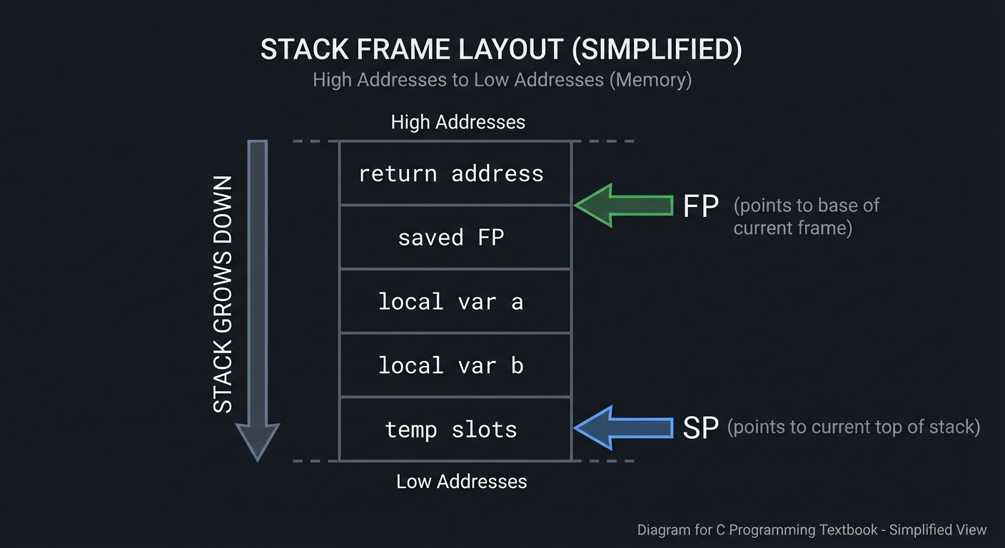
Stack Frame Layout (simplified)

High addresses
| return address |
| saved FP       |
| local var a    |
| local var b    |
| temp slots     |
SP ->            (grows down)
Low addresses

Why Stacks Are Everywhere

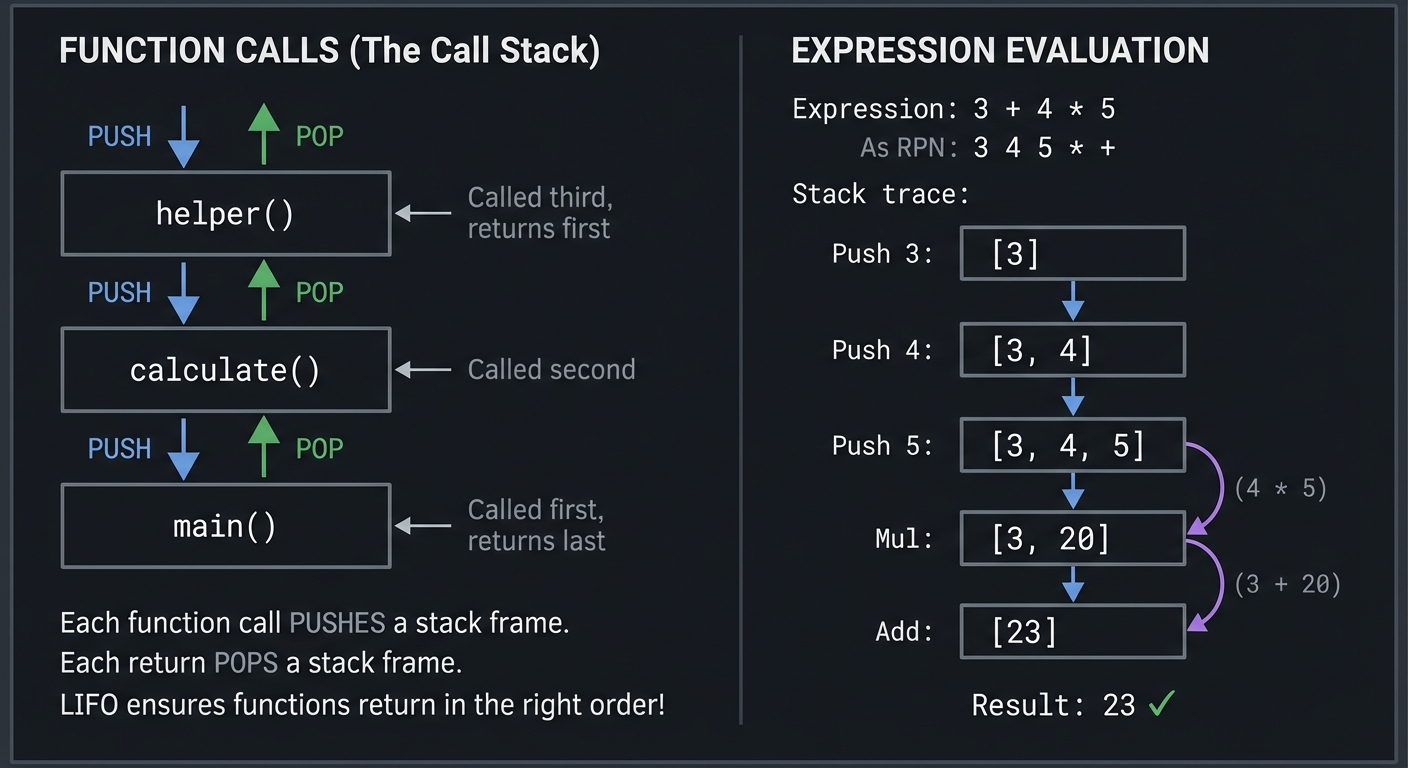
FUNCTION CALLS (The Call Stack):
┌─────────────────┐
│ main()          │ ← Called first, returns last
├─────────────────┤
│ calculate()     │ ← Called second
├─────────────────┤
│ helper()        │ ← Called third, returns first
└─────────────────┘

Each function call PUSHES a stack frame.
Each return POPS a stack frame.
LIFO ensures functions return in the right order!

EXPRESSION EVALUATION:
Expression: 3 + 4 * 5

As RPN: 3 4 5 * +

Stack trace:
  Push 3:     [3]
  Push 4:     [3, 4]
  Push 5:     [3, 4, 5]
  Mul:        [3, 20]      (4 * 5)
  Add:        [23]         (3 + 20)

Result: 23 ✓

---

Project 4: Queue Systems (Task Scheduler & BFS)

• Main Programming Language: C
• Alternative Programming Languages: Rust, Go, Python
• Coolness Level: Level 3: Genuinely Clever
• Business Potential: 2. The “Micro-SaaS / Pro Tool”
• Difficulty: Level 3: Advanced
• Knowledge Area: Abstract Data Types / Systems Programming
• Software or Tool: Job Queue, BFS Maze Solver
• Main Book: Operating Systems: Three Easy Pieces by Remzi H. Arpaci-Dusseau

What you’ll build

A multi-priority task scheduler using queues, plus a visual maze solver using BFS—demonstrating why FIFO (First In, First Out) enables fairness and level-order processing.

Deliverables:

• queue.c/.h with circular buffer implementation
• Multi-level scheduler simulation with time slices
• BFS maze solver with path reconstruction

Why it teaches this concept

Queues are about fairness and ordering:

• First come, first served (FIFO)
• Level-by-level processing (BFS)
• Buffering between producer and consumer

Understanding queues is essential for:

• Operating system schedulers
• Network packet handling
• Message queues (Kafka, RabbitMQ)
• Breadth-first search

Queues are the default structure whenever order and fairness matter.

Core challenges you’ll face

• FIFO semantics (first in, first out) → maps to fairness
• Circular buffer (efficient array-based queue) → maps to memory efficiency
• Priority queues (not FIFO - will connect to heaps) → maps to scheduling
• Producer-consumer (handling different speeds) → maps to buffering
• Fairness vs throughput → maps to system trade-offs

Key Concepts

Concept	Resource
Queue ADT	Introduction to Algorithms Chapter 10.1 - CLRS
Circular Buffers	The Linux Programming Interface Chapter 44 - Kerrisk
BFS Algorithm	Introduction to Algorithms Chapter 22.2 - CLRS
Process Scheduling	Operating Systems: Three Easy Pieces Chapter 7 - OSTEP
Producer/Consumer	Operating Systems: Three Easy Pieces Chapter 30 - OSTEP

Difficulty & Time

• Difficulty: Intermediate
• Time estimate: 1 week
• Prerequisites: Projects 1-3 completed
• Stretch goal: Add a deque and implement 0-1 BFS

Real World Outcome

$ ./task_scheduler

=== Task Scheduler with Multiple Queues ===

Adding tasks:
  [HIGH]   Task: "Handle interrupt"      -> High priority queue
  [MEDIUM] Task: "Process user input"    -> Medium priority queue
  [LOW]    Task: "Background sync"       -> Low priority queue
  [HIGH]   Task: "Memory page fault"     -> High priority queue
  [MEDIUM] Task: "Render frame"          -> Medium priority queue

Processing (high priority first, then FIFO within each level):
  [1] HIGH:   "Handle interrupt"
  [2] HIGH:   "Memory page fault"
  [3] MEDIUM: "Process user input"
  [4] MEDIUM: "Render frame"
  [5] LOW:    "Background sync"

=== BFS Maze Solver ===

Maze:
█████████████
█S    █     █
███ ███ █████
█   █   █   █
█ █████ █ █ █
█       █   █
█████████ ███
█         █E█
█████████████

Solving with BFS...
Step 1: Exploring (1,1) - Added neighbors to queue
Step 2: Exploring (1,2) - Added neighbors to queue
...

Solution found! Path length: 24 steps
█████████████
█S....█.....█
███.███.█████
█...█...█...█
█.█████.█.█.█
█.......█...█
█████████.███
█.........█E█
█████████████

Why BFS finds shortest path: It explores level-by-level!
  Level 0: Start (1,1)
  Level 1: All cells 1 step away
  Level 2: All cells 2 steps away
  ...
  First time we reach End = shortest path!

You should be able to justify why FIFO guarantees the first time you reach a node is the shortest path.

The Core Question You’re Answering

How does FIFO ordering create fairness and shortest-path guarantees, and how do queues model real scheduling systems? What trade-offs appear when you add priorities?

Concepts You Must Understand First

• Queue ADT operations (CLRS, Ch 10.1)
• Circular buffer logic (The Linux Programming Interface, Ch 44)
• BFS and level-order traversal (CLRS, Ch 22.2)
• Scheduling basics (Operating Systems: Three Easy Pieces, Ch 7)
• Producer-consumer queues (Operating Systems: Three Easy Pieces, Ch 30)

Questions to Guide Your Design

• How do you avoid O(n) shifts when dequeuing?
• What does “full” mean in a ring buffer?
• How do you represent multiple priority levels cleanly?
• How do you reconstruct the BFS path?
• How will you avoid starvation in the priority scheduler?

Thinking Exercise

Draw a ring buffer of size 8. Enqueue 6 items, dequeue 4, enqueue 3 more. Track front, rear, and size. Now repeat without using size and see where you get stuck.

The Interview Questions They’ll Ask

• Why does BFS find the shortest path in unweighted graphs?
• How do you implement a queue with two stacks?
• What is the difference between a queue and a deque?
• How would you build a multilevel feedback queue?
• Why is a circular buffer more efficient than shifting an array?
• How would you handle backpressure between producer and consumer?

Hints in Layers

1) Implement a fixed-size queue with front, rear, and size. 2) Add modulo arithmetic for wrap-around. 3) Build multiple queues for priority scheduling. 4) For BFS, track parents to reconstruct the path. 5) Add a simple aging mechanism to avoid starvation.

q->rear = (q->rear + 1) % QUEUE_CAPACITY;
q->front = (q->front + 1) % QUEUE_CAPACITY;

Books That Will Help

Topic	Book	Why It Helps
Queue ADT	CLRS, Ch 10.1	Formal operations
Circular buffers	The Linux Programming Interface, Ch 44	Practical ring buffers
BFS	CLRS, Ch 22.2	Correctness of BFS
Scheduling	Operating Systems: Three Easy Pieces, Ch 7	Real systems context
Concurrency	Operating Systems: Three Easy Pieces, Ch 30	Producer/consumer patterns

Common Pitfalls & Debugging

Problem: “Queue appears full when it is not”

• Why: front and rear wrap incorrectly.
• Fix: Track size explicitly or keep one empty slot.
• Quick test: Enqueue/dequeue in a loop of 1000 ops.

Problem: “BFS path is wrong”

• Why: Parent pointers not set for every visited node.
• Fix: Set parent when enqueuing, not when dequeuing.
• Quick test: Compare path length with distance array.

Problem: “Priority queue starves low tasks”

• Why: Strict priority scheduling without aging.
• Fix: Add aging or round-robin per priority.
• Quick test: Run 100 high tasks and ensure low tasks eventually run.

Problem: “BFS revisits nodes”

• Why: Visited set not updated on enqueue.
• Fix: Mark visited as soon as you enqueue.
• Quick test: Run BFS on a cyclic graph and verify no infinite loop.

Definition of Done

• Circular buffer queue passes wrap-around tests
• Task scheduler respects priority and FIFO within levels
• BFS finds shortest path and prints it
• Queue invariants checked after each op
• Stress tests run without overflow or underflow errors
• Starvation avoidance tested with aging

Learning Milestones

1. Basic queue works → You understand FIFO
2. Circular buffer is efficient → You understand wrapping
3. Priority scheduler works → You understand scheduling
4. BFS finds shortest path → You understand level-order processing
5. Fairness is visible → You can reason about starvation

Implementation

Queue with Circular Buffer

#define QUEUE_CAPACITY 100

typedef struct {
    int items[QUEUE_CAPACITY];
    int front;      // Index to dequeue from
    int rear;       // Index to enqueue to
    int size;
} Queue;

void queue_init(Queue* q) {
    q->front = 0;
    q->rear = 0;
    q->size = 0;
}

int queue_is_empty(Queue* q) {
    return q->size == 0;
}

int queue_is_full(Queue* q) {
    return q->size == QUEUE_CAPACITY;
}

void queue_enqueue(Queue* q, int value) {
    if (queue_is_full(q)) {
        printf("Queue overflow!\n");
        return;
    }
    q->items[q->rear] = value;
    q->rear = (q->rear + 1) % QUEUE_CAPACITY;  // Wrap around!
    q->size++;
}

int queue_dequeue(Queue* q) {
    if (queue_is_empty(q)) {
        printf("Queue underflow!\n");
        return -1;
    }
    int value = q->items[q->front];
    q->front = (q->front + 1) % QUEUE_CAPACITY;  // Wrap around!
    q->size--;
    return value;
}

// Visualize circular buffer
void queue_visualize(Queue* q) {
    printf("Queue (front=%d, rear=%d, size=%d):\n[", q->front, q->rear, q->size);
    for (int i = 0; i < QUEUE_CAPACITY && i < 20; i++) {
        if (i >= q->front && i < q->front + q->size) {
            printf("%d", q->items[i % QUEUE_CAPACITY]);
        } else {
            printf("_");
        }
        if (i < 19) printf(",");
    }
    printf("...]\n");
}

Multi-Level Priority Scheduler

typedef enum { HIGH, MEDIUM, LOW, NUM_PRIORITIES } Priority;

typedef struct {
    char name[64];
    Priority priority;
} Task;

typedef struct {
    Queue queues[NUM_PRIORITIES];
    Task tasks[1000];  // Task storage
    int task_count;
} Scheduler;

void scheduler_add_task(Scheduler* s, const char* name, Priority priority) {
    Task* task = &s->tasks[s->task_count];
    strcpy(task->name, name);
    task->priority = priority;

    // Add task index to appropriate queue
    queue_enqueue(&s->queues[priority], s->task_count);
    s->task_count++;

    const char* priority_names[] = {"HIGH", "MEDIUM", "LOW"};
    printf("Added [%s] task: \"%s\"\n", priority_names[priority], name);
}

Task* scheduler_get_next(Scheduler* s) {
    // Check high priority first, then medium, then low
    for (int p = HIGH; p < NUM_PRIORITIES; p++) {
        if (!queue_is_empty(&s->queues[p])) {
            int task_idx = queue_dequeue(&s->queues[p]);
            return &s->tasks[task_idx];
        }
    }
    return NULL;  // No tasks
}

BFS Maze Solver

#define MAZE_SIZE 13

typedef struct {
    int row, col;
    int distance;
} Cell;

int bfs_solve_maze(char maze[MAZE_SIZE][MAZE_SIZE],
                   int start_row, int start_col,
                   int end_row, int end_col) {

    // Queue for BFS
    Cell queue[MAZE_SIZE * MAZE_SIZE];
    int front = 0, rear = 0;

    // Visited array
    int visited[MAZE_SIZE][MAZE_SIZE] = {0};

    // Parent tracking for path reconstruction
    int parent_row[MAZE_SIZE][MAZE_SIZE];
    int parent_col[MAZE_SIZE][MAZE_SIZE];

    // Start BFS
    queue[rear++] = (Cell){start_row, start_col, 0};
    visited[start_row][start_col] = 1;

    int directions[4][2] = {{-1, 0}, {1, 0}, {0, -1}, {0, 1}};

    while (front < rear) {
        Cell current = queue[front++];

        // Found the end!
        if (current.row == end_row && current.col == end_col) {
            // Reconstruct path
            int r = end_row, c = end_col;
            while (r != start_row || c != start_col) {
                maze[r][c] = '.';
                int pr = parent_row[r][c];
                int pc = parent_col[r][c];
                r = pr;
                c = pc;
            }
            maze[start_row][start_col] = 'S';
            maze[end_row][end_col] = 'E';
            return current.distance;
        }

        // Explore neighbors
        for (int d = 0; d < 4; d++) {
            int nr = current.row + directions[d][0];
            int nc = current.col + directions[d][1];

            if (nr >= 0 && nr < MAZE_SIZE && nc >= 0 && nc < MAZE_SIZE &&
                maze[nr][nc] != '#' && !visited[nr][nc]) {

                visited[nr][nc] = 1;
                parent_row[nr][nc] = current.row;
                parent_col[nr][nc] = current.col;
                queue[rear++] = (Cell){nr, nc, current.distance + 1};
            }
        }
    }

    return -1;  // No path found
}

Design Notes

• Use a ring buffer to keep enqueue/dequeue O(1).
• Track size explicitly to disambiguate full vs empty.
• For BFS, mark nodes visited when enqueued, not when dequeued.
• Keep scheduler queues separate to enforce strict priority.

Testing & Validation

• Enqueue/dequeue in a loop of 10,000 ops and verify order.
• Verify BFS path length against a known shortest path.
• Test scheduler fairness with mixed priority loads.

Performance Experiments

• Compare array-shift queue vs ring buffer for 100k ops.
• Measure BFS runtime on sparse vs dense grids.
• Measure scheduler throughput with high-priority spikes.

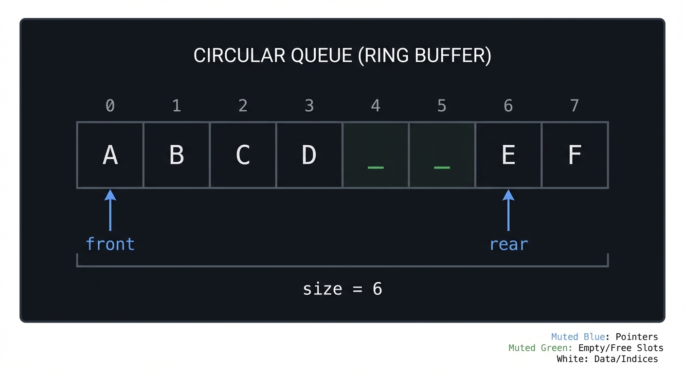
Queue Ring Buffer (capacity=8)

index: 0 1 2 3 4 5 6 7
data:  A B C D _ _ E F
front -> 0
rear  -> 6 (next insert)
size  -> 6

Stack vs Queue: When to Use Each

Use Case	Stack (LIFO)	Queue (FIFO)
Undo/Redo	✓
Function calls	✓
DFS traversal	✓
Expression evaluation	✓
Task scheduling		✓
BFS traversal		✓
Print queue		✓
Message buffering		✓

Key insight:

• Stack: When most recent is most important
• Queue: When order of arrival matters (fairness)

---

Project 5: Hash Table (Dictionary & Cache)

• Main Programming Language: C
• Alternative Programming Languages: Rust, Python, Go
• Coolness Level: Level 4: Hardcore Tech Flex
• Business Potential: 4. The “Open Core” Infrastructure
• Difficulty: Level 4: Expert
• Knowledge Area: Data Structures / Algorithms
• Software or Tool: Key-Value Store, LRU Cache
• Main Book: Introduction to Algorithms by CLRS

What you’ll build

A complete hash table implementation with multiple collision resolution strategies (chaining, open addressing), plus a practical LRU (Least Recently Used) cache.

Deliverables:

• hash_chaining.c and hash_open.c
• Benchmark script comparing probe lengths and collisions
• lru_cache.c with O(1) get/put

Why it teaches this concept

Hash tables are the most practically important data structure:

• O(1) average lookup, insert, delete
• Backbone of databases, caches, dictionaries
• Used everywhere: Python dicts, JavaScript objects, database indexes

Understanding hash tables means understanding:

• Hash functions (turning keys into indices)
• Collision resolution (when two keys hash to same index)
• Load factor and resizing
• Trade-offs between time and space

This project also teaches you why “average O(1)” depends on your hash quality and resize policy.

Core challenges you’ll face

• Hash function design (distribute keys uniformly) → maps to hashing theory
• Collision handling (chaining vs open addressing) → maps to trade-offs
• Load factor (when to resize) → maps to performance tuning
• LRU eviction (combining hash table with linked list) → maps to real caches
• Probe clustering (open addressing) → maps to performance degradation

Resources for Key Challenges

• Real-world Applications of Hash Tables - Practical use cases
• GeeksforGeeks: Real-life Applications of DSA - Hash tables in databases, caching

Key Concepts

Concept	Resource
Hash Functions	Introduction to Algorithms Chapter 11 - CLRS
Collision Resolution	Algorithms, Fourth Edition Chapter 3.4 - Sedgewick
Universal Hashing	Introduction to Algorithms Chapter 11.3.3 - CLRS
LRU Cache Design	LeetCode Problem 146 explanation
Hash tables in C	Mastering Algorithms with C Chapter 8

Difficulty & Time

• Difficulty: Advanced
• Time estimate: 2 weeks
• Prerequisites: Projects 1-2 completed, understanding of modular arithmetic
• Stretch goal: Add robin hood hashing

Real World Outcome

$ ./hashtable_demo

=== Hash Table with Chaining ===
Initial capacity: 16, load factor threshold: 0.75

put("apple", 5)   -> hash("apple") = 7, bucket 7
put("banana", 3)  -> hash("banana") = 2, bucket 2
put("cherry", 8)  -> hash("cherry") = 7, bucket 7 (collision with apple!)

Bucket visualization:
[0]: empty
[1]: empty
[2]: ["banana" -> 3]
...
[7]: ["apple" -> 5] -> ["cherry" -> 8]  ← Chained!
...

get("cherry") = 8  (found in bucket 7, 2nd in chain)
get("mango") = NOT FOUND

=== Open Addressing (Linear Probing) ===
put("apple", 5)   -> hash = 7, slot 7
put("cherry", 8)  -> hash = 7, collision! probe slot 8

Table visualization:
[0]: empty
...
[7]: ("apple", 5)
[8]: ("cherry", 8)  ← Probed here!
...

=== Resize Demo ===
Adding 12 items... load factor = 0.75
RESIZE triggered! 16 -> 32 buckets
All items rehashed to new positions

=== LRU Cache (capacity=3) ===
put(1, "one")    Cache: [1]
put(2, "two")    Cache: [2, 1]
put(3, "three")  Cache: [3, 2, 1]
get(1)           Cache: [1, 3, 2]  ← 1 moved to front (recently used)
put(4, "four")   Cache: [4, 1, 3]  ← 2 evicted (least recently used)!
get(2)           MISS! (was evicted)

You should be able to print average probe lengths and show how they change with load factor.

The Core Question You’re Answering

How do you turn arbitrary keys into near-constant-time lookup, and what do you do when keys collide? How do you choose a resizing strategy that stays fast under load?

Concepts You Must Understand First

• Hash function basics (CLRS, Ch 11)
• Collision resolution strategies (Algorithms, Fourth Edition, Ch 3.4)
• Load factor and resizing (CLRS, Ch 11.5)
• Doubly linked list for LRU (CLRS, Ch 10)
• Tombstones and deletions in open addressing (Algorithms, Fourth Edition, Ch 3.4)

Questions to Guide Your Design

• What makes a hash function “good” for your key type?
• How will you trigger resize and rehashing?
• Do you want chaining or open addressing, and why?
• How will you track recency for LRU in O(1)?
• How will you measure and report collision rates?

Thinking Exercise

Pick 10 strings and compute their hash buckets for a 16-slot table. Count collisions and think about how to reduce them. Repeat with a different hash function and compare.

The Interview Questions They’ll Ask

• Why are hash tables O(1) on average but O(n) worst case?
• What is a load factor and how does it affect performance?
• What are the trade-offs between chaining and open addressing?
• How do you design an LRU cache with O(1) operations?
• What happens if you use a poor hash function?
• Why are hash tables hard to make thread-safe?

Hints in Layers

1) Implement a simple chaining hash table first. 2) Add load factor checks and resize by doubling capacity. 3) Implement open addressing with linear probing as a second mode. 4) Combine hash table + doubly linked list for LRU. 5) Log average probe length as you insert many keys.

float load = (float)ht->size / ht->capacity;
if (load > ht->max_load_factor) ht_resize(ht, ht->capacity * 2);

Books That Will Help

Topic	Book	Why It Helps
Hashing	CLRS, Ch 11	Theory and practice
Open addressing	Algorithms, Fourth Edition, Ch 3.4	Implementation details
LRU design	Mastering Algorithms with C, Ch 10	Cache patterns
Practical hashing	Algorithms in C, Parts 1-4	C-specific patterns

Common Pitfalls & Debugging

Problem: “Hash table gets slower over time”

• Why: Resize never happens or load factor too high.
• Fix: Resize earlier and test with large input sets.
• Quick test: Insert 1M keys and track average probe length.

Problem: “Keys disappear after resize”

• Why: Rehash step missing or incorrect.
• Fix: Re-insert every entry into new buckets.
• Quick test: Insert N keys, resize, then verify all N lookups.

Problem: “LRU ordering is wrong”

• Why: List links not updated on access.
• Fix: Move node to head on every get and put.
• Quick test: Access a key and ensure it becomes most recent.

Problem: “Open addressing never finds key”

• Why: Tombstones not handled correctly.
• Fix: Treat DELETED slots as occupied for search, free for insert.
• Quick test: Insert, delete, and re-insert same key.

Definition of Done

• Chaining and open addressing implementations both work
• Resize keeps load factor under threshold
• LRU cache supports get/put in O(1)
• Collision counts and probe lengths are tracked
• All operations pass randomized tests
• Hash distribution test shows near-uniform buckets

Learning Milestones

1. Hash function distributes evenly → You understand hashing
2. Chaining handles collisions → You understand linked lists in practice
3. Open addressing works → You understand the alternative trade-off
4. Resize maintains O(1) amortized → You understand load factors
5. LRU cache works → You understand combining data structures
6. Probe statistics make sense → You understand clustering

Implementation

Hash Function

// DJB2 hash - simple and effective
uint32_t hash_string(const char* str) {
    uint32_t hash = 5381;
    int c;
    while ((c = *str++)) {
        hash = ((hash << 5) + hash) + c;  // hash * 33 + c
    }
    return hash;
}

// For integer keys
uint32_t hash_int(int key) {
    // Knuth's multiplicative hash
    return key * 2654435761u;
}

Hash Table with Chaining

typedef struct Entry {
    char* key;
    int value;
    struct Entry* next;  // For chaining
} Entry;

typedef struct {
    Entry** buckets;     // Array of linked lists
    size_t capacity;
    size_t size;
    float max_load_factor;
} HashTable;

HashTable* ht_create(size_t capacity) {
    HashTable* ht = malloc(sizeof(HashTable));
    ht->buckets = calloc(capacity, sizeof(Entry*));
    ht->capacity = capacity;
    ht->size = 0;
    ht->max_load_factor = 0.75;
    return ht;
}

void ht_put(HashTable* ht, const char* key, int value) {
    // Check load factor
    float load = (float)ht->size / ht->capacity;
    if (load > ht->max_load_factor) {
        ht_resize(ht, ht->capacity * 2);
    }

    uint32_t hash = hash_string(key);
    size_t index = hash % ht->capacity;

    // Check if key exists
    Entry* entry = ht->buckets[index];
    while (entry) {
        if (strcmp(entry->key, key) == 0) {
            entry->value = value;  // Update
            return;
        }
        entry = entry->next;
    }

    // Insert new entry at head of chain
    Entry* new_entry = malloc(sizeof(Entry));
    new_entry->key = strdup(key);
    new_entry->value = value;
    new_entry->next = ht->buckets[index];
    ht->buckets[index] = new_entry;
    ht->size++;
}

int ht_get(HashTable* ht, const char* key, int* found) {
    uint32_t hash = hash_string(key);
    size_t index = hash % ht->capacity;

    Entry* entry = ht->buckets[index];
    while (entry) {
        if (strcmp(entry->key, key) == 0) {
            *found = 1;
            return entry->value;
        }
        entry = entry->next;
    }

    *found = 0;
    return 0;
}

void ht_resize(HashTable* ht, size_t new_capacity) {
    Entry** old_buckets = ht->buckets;
    size_t old_capacity = ht->capacity;

    ht->buckets = calloc(new_capacity, sizeof(Entry*));
    ht->capacity = new_capacity;
    ht->size = 0;

    // Rehash all entries
    for (size_t i = 0; i < old_capacity; i++) {
        Entry* entry = old_buckets[i];
        while (entry) {
            Entry* next = entry->next;
            ht_put(ht, entry->key, entry->value);
            free(entry->key);
            free(entry);
            entry = next;
        }
    }

    free(old_buckets);
    printf("Resized: %zu -> %zu buckets\n", old_capacity, new_capacity);
}

Hash Table with Open Addressing (Linear Probing)

typedef enum { EMPTY, OCCUPIED, DELETED } SlotState;

typedef struct {
    char* key;
    int value;
    SlotState state;
} Slot;

typedef struct {
    Slot* slots;
    size_t capacity;
    size_t size;
} OpenHashTable;

void oht_put(OpenHashTable* ht, const char* key, int value) {
    uint32_t hash = hash_string(key);
    size_t index = hash % ht->capacity;

    // Linear probing
    size_t start = index;
    do {
        if (ht->slots[index].state == EMPTY ||
            ht->slots[index].state == DELETED) {
            // Found empty slot
            ht->slots[index].key = strdup(key);
            ht->slots[index].value = value;
            ht->slots[index].state = OCCUPIED;
            ht->size++;
            return;
        }

        if (ht->slots[index].state == OCCUPIED &&
            strcmp(ht->slots[index].key, key) == 0) {
            // Key exists - update
            ht->slots[index].value = value;
            return;
        }

        index = (index + 1) % ht->capacity;  // Probe next slot
    } while (index != start);

    printf("Hash table full!\n");
}

LRU Cache (Hash Table + Doubly Linked List)

typedef struct LRUNode {
    int key;
    int value;
    struct LRUNode* prev;
    struct LRUNode* next;
} LRUNode;

typedef struct {
    int capacity;
    int size;
    LRUNode* head;          // Most recently used
    LRUNode* tail;          // Least recently used
    LRUNode** hash_table;   // For O(1) lookup
    int table_size;
} LRUCache;

void lru_move_to_front(LRUCache* cache, LRUNode* node) {
    if (node == cache->head) return;

    // Remove from current position
    if (node->prev) node->prev->next = node->next;
    if (node->next) node->next->prev = node->prev;
    if (node == cache->tail) cache->tail = node->prev;

    // Insert at head
    node->prev = NULL;
    node->next = cache->head;
    if (cache->head) cache->head->prev = node;
    cache->head = node;
    if (!cache->tail) cache->tail = node;
}

int lru_get(LRUCache* cache, int key) {
    int index = key % cache->table_size;
    LRUNode* node = cache->hash_table[index];

    // Find in chain
    while (node && node->key != key) {
        node = node->next;  // Actually need separate chaining here
    }

    if (!node) return -1;  // Not found

    // Move to front (mark as recently used)
    lru_move_to_front(cache, node);
    return node->value;
}

void lru_put(LRUCache* cache, int key, int value) {
    // Check if exists
    int index = key % cache->table_size;
    LRUNode* existing = cache->hash_table[index];

    if (existing) {
        existing->value = value;
        lru_move_to_front(cache, existing);
        return;
    }

    // Check if at capacity
    if (cache->size >= cache->capacity) {
        // Evict LRU (tail)
        LRUNode* victim = cache->tail;
        printf("Evicting key %d (LRU)\n", victim->key);

        // Remove from hash table
        int victim_index = victim->key % cache->table_size;
        cache->hash_table[victim_index] = NULL;

        // Remove from list
        cache->tail = victim->prev;
        if (cache->tail) cache->tail->next = NULL;
        free(victim);
        cache->size--;
    }

    // Add new node
    LRUNode* node = malloc(sizeof(LRUNode));
    node->key = key;
    node->value = value;
    node->prev = NULL;
    node->next = cache->head;

    if (cache->head) cache->head->prev = node;
    cache->head = node;
    if (!cache->tail) cache->tail = node;

    cache->hash_table[index] = node;
    cache->size++;
}

Design Notes

• Choose a hash function appropriate for key types (strings vs ints).
• Keep load factor thresholds conservative for open addressing.
• For LRU, use a hash table for lookup and a doubly linked list for order.
• Consider storing hash values to avoid recomputation in chains.

Testing & Validation

• Insert N keys, then verify all lookups succeed after resize.
• Delete and reinsert keys to validate tombstone handling.
• Verify LRU order after repeated access patterns.

Performance Experiments

• Track average chain length or probe length vs load factor.
• Benchmark chaining vs linear probing for random vs clustered keys.
• Measure LRU hit ratio under skewed access distributions.

Collision Strategies (bucket 7)

Chaining:
[7] -> ("apple") -> ("cherry") -> NULL

Open Addressing (linear probing):
index 7: ("apple")
index 8: ("cherry")
index 9: empty

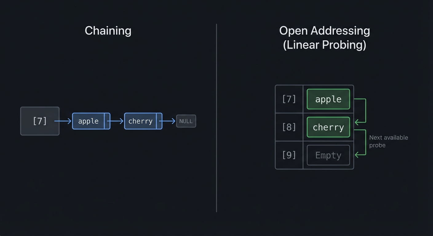
Chaining vs Open Addressing

Aspect	Chaining	Open Addressing
Memory	Pointer overhead per entry	No extra pointers
Cache	Poor (linked list traversal)	Good (contiguous probing)
Load factor	Can exceed 1.0	Must stay below ~0.7
Deletion	Simple (unlink node)	Complex (tombstones)
Implementation	Easier	Harder
Clustering	No	Yes (performance degrades)

---

Project 6: Binary Search Tree & Balancing

• Main Programming Language: C
• Alternative Programming Languages: Rust, Go, Java
• Coolness Level: Level 4: Hardcore Tech Flex
• Business Potential: 1. The “Resume Gold”
• Difficulty: Level 4: Expert
• Knowledge Area: Trees / Self-Balancing
• Software or Tool: BST with visualization, AVL Tree
• Main Book: Introduction to Algorithms by CLRS

What you’ll build

A binary search tree with visualization, then extend it to a self-balancing AVL tree, demonstrating why balancing is crucial for performance.

Deliverables:

• bst.c/.h with insert/search/delete/traverse
• avl.c/.h with rotations and height tracking
• Tree visualization utility

Why it teaches this concept

Trees enable O(log n) operations when balanced:

• Searching
• Insertion
• Deletion
• Range queries
• Ordered traversal

But an unbalanced tree degrades to O(n)—essentially a linked list. Understanding balancing is crucial for:

• Database indexes (B-trees)
• File systems
• Memory allocators (red-black trees in Linux kernel)
• Priority scheduling

Balanced trees are the bridge between array-like speed and linked-list flexibility.

Core challenges you’ll face

• BST property (left < node < right) → maps to binary search
• Tree traversal (in-order, pre-order, post-order) → maps to recursive thinking
• Deletion (three cases: leaf, one child, two children) → maps to pointer manipulation
• Balancing (rotations to maintain height) → maps to self-balancing
• Height maintenance (update on every insert/delete) → maps to invariants

Key Concepts

Concept	Resource
BST Operations	Introduction to Algorithms Chapter 12 - CLRS
Tree Traversals	Algorithms, Fourth Edition Chapter 3.2 - Sedgewick
AVL Trees	Introduction to Algorithms Chapter 13 (similar to RB trees) - CLRS
Rotations	Visualgo.net BST visualization
Tree invariants	Mastering Algorithms with C Chapter 4

Difficulty & Time

• Difficulty: Advanced
• Time estimate: 2 weeks
• Prerequisites: Projects 1-4 completed, recursion comfort
• Stretch goal: Add a red-black tree variant

Real World Outcome

$ ./bst_demo

=== Binary Search Tree Demo ===
Inserting: 50, 30, 70, 20, 40, 60, 80

Tree visualization:
         50
        /  \
      30    70
     /  \  /  \
   20  40 60  80

In-order traversal (sorted!): 20 30 40 50 60 70 80
Tree height: 3
Is balanced: YES

=== Unbalanced Insertion Demo ===
Inserting sorted: 10, 20, 30, 40, 50, 60, 70

Tree visualization:
10
  \
   20
     \
      30
        \
         40
           \
            50 ... (degenerates to linked list!)

Height: 7 (should be 3 for balanced)
Is balanced: NO
Search for 70: 7 comparisons (should be 3!)

=== AVL Tree (Self-Balancing) ===
Same insertions: 10, 20, 30, 40, 50, 60, 70

After each insert, rebalance:
Insert 10:     10
Insert 20:     10-20
Insert 30:     10-20-30 -> ROTATE LEFT
                 20
                /  \
              10   30
Insert 40:       20
                /  \
              10   30-40
Insert 50:       20           30
                /  \    ->   /  \
              10   30-40-50  20  40
                            /     \
                          10      50
...

Final AVL tree:
         40
        /  \
      20    60
     /  \  /  \
   10  30 50  70

Height: 3 (optimal!)
All operations: O(log n) guaranteed!

You should be able to show that the AVL height stays within a small constant factor of log2(n).

The Core Question You’re Answering

How do you keep ordered data fast to search, and why does balancing prevent worst-case slowdown? What rotations restore invariants after updates?

Concepts You Must Understand First

• BST property and traversal orders (CLRS, Ch 12)
• Tree height and balance (CLRS, Ch 13)
• Rotations and invariants (CLRS, Ch 13)
• Recursion and stack frames (The Recursive Book of Recursion, Ch 1-3)
• Binary tree representation in memory (Mastering Algorithms with C, Ch 4)

Questions to Guide Your Design

• How will you handle duplicate keys?
• What is the exact rotation logic for all four AVL cases?
• How do you compute and update node heights correctly?
• How will you visualize the tree after each insertion?
• How will you test that traversal results are always sorted?

Thinking Exercise

Insert the sequence 30, 20, 10 into a BST. Draw the tree and then show how a right rotation restores balance. Repeat for 10, 30, 20 (left-right case).

The Interview Questions They’ll Ask

• Why can a BST degrade to O(n)?
• What is the difference between AVL and red-black trees?
• How does in-order traversal produce sorted output?
• What are the three BST delete cases?
• Why are B-trees used on disk instead of BSTs?
• How do you implement range queries efficiently?

Hints in Layers

1) Implement a plain BST insert/search first. 2) Add a height field and compute balance factor. 3) Implement rotations and test them in isolation. 4) Plug rotations into insert and verify balance after each insert. 5) Add unit tests that insert sorted data and check height.

int balance = get_balance(root);
if (balance > 1 && key < root->left->key) return rotate_right(root);
if (balance < -1 && key > root->right->key) return rotate_left(root);

Books That Will Help

Topic	Book	Why It Helps
BSTs	CLRS, Ch 12	Core operations
Balancing	CLRS, Ch 13	Rotations and invariants
Trees in C	Mastering Algorithms with C, Ch 4-5	Practical C details
Recursion intuition	The Recursive Book of Recursion, Ch 1-3	Tree traversal reasoning

Common Pitfalls & Debugging

Problem: “Tree becomes unbalanced after insert”

• Why: Height updates happen before rotation or on wrong node.
• Fix: Update heights bottom-up after insertion.
• Quick test: Insert ascending keys and check height.

Problem: “Delete loses subtrees”

• Why: Incorrect successor replacement.
• Fix: Use in-order successor and reattach children carefully.
• Quick test: Delete root in a 7-node tree and verify all nodes remain.

Problem: “Traversal prints wrong order”

• Why: In-order traversal implemented incorrectly.
• Fix: Always do left, root, right.
• Quick test: Insert 1..5 and ensure output is sorted.

Problem: “Heights drift over time”

• Why: Height updates only on inserts, not deletes.
• Fix: Update height on every modification.
• Quick test: Insert then delete and validate heights.

Definition of Done

• BST insert/search/delete pass unit tests
• AVL insert keeps height within 1 for all nodes
• Tree visualizer prints correct structure
• Range queries and in-order traversal produce correct order
• Performance is O(log n) on random inserts
• Rotation tests cover LL, RR, LR, RL cases

Learning Milestones

1. BST insertion/search works → You understand the BST property
2. In-order traversal is sorted → You understand tree ordering
3. Unbalanced tree is slow → You understand why balancing matters
4. AVL rotations fix balance → You understand self-balancing
5. Delete preserves invariants → You understand complex edge cases

Implementation

Basic BST

typedef struct TreeNode {
    int key;
    struct TreeNode* left;
    struct TreeNode* right;
    int height;  // For AVL
} TreeNode;

TreeNode* create_node(int key) {
    TreeNode* node = malloc(sizeof(TreeNode));
    node->key = key;
    node->left = NULL;
    node->right = NULL;
    node->height = 1;
    return node;
}

// O(h) where h is height
TreeNode* bst_insert(TreeNode* root, int key) {
    if (root == NULL) {
        return create_node(key);
    }

    if (key < root->key) {
        root->left = bst_insert(root->left, key);
    } else if (key > root->key) {
        root->right = bst_insert(root->right, key);
    }
    // If equal, ignore (no duplicates)

    return root;
}

// O(h) where h is height
TreeNode* bst_search(TreeNode* root, int key, int* comparisons) {
    (*comparisons)++;

    if (root == NULL || root->key == key) {
        return root;
    }

    if (key < root->key) {
        return bst_search(root->left, key, comparisons);
    } else {
        return bst_search(root->right, key, comparisons);
    }
}

// In-order: Left, Root, Right -> Sorted order!
void inorder_traversal(TreeNode* root) {
    if (root == NULL) return;
    inorder_traversal(root->left);
    printf("%d ", root->key);
    inorder_traversal(root->right);
}

// Find minimum (leftmost node)
TreeNode* find_min(TreeNode* root) {
    while (root->left) {
        root = root->left;
    }
    return root;
}

// Deletion (the tricky one!)
TreeNode* bst_delete(TreeNode* root, int key) {
    if (root == NULL) return NULL;

    if (key < root->key) {
        root->left = bst_delete(root->left, key);
    } else if (key > root->key) {
        root->right = bst_delete(root->right, key);
    } else {
        // Found the node to delete

        // Case 1: Leaf node
        if (!root->left && !root->right) {
            free(root);
            return NULL;
        }

        // Case 2: One child
        if (!root->left) {
            TreeNode* temp = root->right;
            free(root);
            return temp;
        }
        if (!root->right) {
            TreeNode* temp = root->left;
            free(root);
            return temp;
        }

        // Case 3: Two children
        // Find in-order successor (smallest in right subtree)
        TreeNode* successor = find_min(root->right);
        root->key = successor->key;
        root->right = bst_delete(root->right, successor->key);
    }

    return root;
}

Tree Visualization

void print_tree_helper(TreeNode* root, int space, int height) {
    if (root == NULL) return;

    space += height;

    print_tree_helper(root->right, space, height);

    printf("\n");
    for (int i = height; i < space; i++) {
        printf(" ");
    }
    printf("%d\n", root->key);

    print_tree_helper(root->left, space, height);
}

void print_tree(TreeNode* root) {
    print_tree_helper(root, 0, 5);
}

int tree_height(TreeNode* root) {
    if (root == NULL) return 0;
    int left_h = tree_height(root->left);
    int right_h = tree_height(root->right);
    return 1 + (left_h > right_h ? left_h : right_h);
}

int is_balanced(TreeNode* root) {
    if (root == NULL) return 1;

    int left_h = tree_height(root->left);
    int right_h = tree_height(root->right);

    if (abs(left_h - right_h) > 1) return 0;

    return is_balanced(root->left) && is_balanced(root->right);
}

AVL Tree (Self-Balancing)

int get_height(TreeNode* node) {
    return node ? node->height : 0;
}

int get_balance(TreeNode* node) {
    return node ? get_height(node->left) - get_height(node->right) : 0;
}

void update_height(TreeNode* node) {
    int left_h = get_height(node->left);
    int right_h = get_height(node->right);
    node->height = 1 + (left_h > right_h ? left_h : right_h);
}

// Right rotation
//       y                x
//      / \              / \
//     x   C    ->      A   y
//    / \                  / \
//   A   B                B   C
TreeNode* rotate_right(TreeNode* y) {
    TreeNode* x = y->left;
    TreeNode* B = x->right;

    x->right = y;
    y->left = B;

    update_height(y);
    update_height(x);

    return x;
}

// Left rotation
TreeNode* rotate_left(TreeNode* x) {
    TreeNode* y = x->right;
    TreeNode* B = y->left;

    y->left = x;
    x->right = B;

    update_height(x);
    update_height(y);

    return y;
}

TreeNode* avl_insert(TreeNode* root, int key) {
    // Standard BST insert
    if (root == NULL) {
        return create_node(key);
    }

    if (key < root->key) {
        root->left = avl_insert(root->left, key);
    } else if (key > root->key) {
        root->right = avl_insert(root->right, key);
    } else {
        return root;  // No duplicates
    }

    // Update height
    update_height(root);

    // Check balance
    int balance = get_balance(root);

    // Left Left Case
    if (balance > 1 && key < root->left->key) {
        printf("Left-Left case: rotating right\n");
        return rotate_right(root);
    }

    // Right Right Case
    if (balance < -1 && key > root->right->key) {
        printf("Right-Right case: rotating left\n");
        return rotate_left(root);
    }

    // Left Right Case
    if (balance > 1 && key > root->left->key) {
        printf("Left-Right case: double rotation\n");
        root->left = rotate_left(root->left);
        return rotate_right(root);
    }

    // Right Left Case
    if (balance < -1 && key < root->right->key) {
        printf("Right-Left case: double rotation\n");
        root->right = rotate_right(root->right);
        return rotate_left(root);
    }

    return root;
}

Design Notes

• Keep rotation helpers small and testable in isolation.
• Update heights after every structural change.
• Decide a policy for duplicates early (ignore, count, or store list).
• Provide traversal helpers for debugging and validation.

Testing & Validation

• Insert sorted input and verify height remains O(log n).
• Trigger each rotation case (LL, RR, LR, RL) with small sequences.
• Validate in-order traversal output after every insert/delete.

Performance Experiments

• Compare search times for balanced vs unbalanced trees.
• Measure rotation counts for random vs sorted insertions.
• Benchmark range queries on BST vs hash table.

AVL Rotation Cases (schematic)

LL:        y            x
          / \          / \
         x   C  ->    A   y
        / \              / \
       A   B            B   C

RR:        y            x
          / \          / \
         A   x  ->    y   C
            / \      / \
           B   C    A   B

BST vs Hash Table

Operation	Hash Table	BST (balanced)	BST (unbalanced)
Search	O(1) avg	O(log n)	O(n)
Insert	O(1) avg	O(log n)	O(n)
Delete	O(1) avg	O(log n)	O(n)
Ordered traversal	O(n log n) sort	O(n)	O(n)
Range query	O(n)	O(log n + k)	O(n)
Min/Max	O(n)	O(log n)	O(n)

Use BST when:

• You need ordered data
• Range queries are common
• You need min/max quickly

Use Hash Table when:

• Order doesn’t matter
• Just need fast lookup by key

---

Project 7: Heap & Priority Queue

• Main Programming Language: C
• Alternative Programming Languages: Rust, Python, Go
• Coolness Level: Level 3: Genuinely Clever
• Business Potential: 2. The “Micro-SaaS / Pro Tool”
• Difficulty: Level 3: Advanced
• Knowledge Area: Heaps / Priority Queues
• Software or Tool: Task scheduler, Heapsort visualizer
• Main Book: Introduction to Algorithms by CLRS

What you’ll build

A binary heap (min and max), priority queue, and heapsort implementation with visualization—plus a practical task scheduler that always runs the highest-priority task.

Deliverables:

• heap.c/.h with insert, extract, build
• heapsort.c benchmark
• Priority queue scheduler demo

Why it teaches this concept

Heaps answer the question: What if I only care about the minimum (or maximum)?

A BST gives O(log n) for everything, but requires balancing. A heap gives:

• O(1) find-min
• O(log n) insert
• O(log n) extract-min

And it’s simpler to implement (just an array!). Heaps are used in:

• Priority scheduling (OS, network packets)
• Dijkstra’s algorithm (shortest path)
• Heap sort (in-place O(n log n))
• Merge k sorted lists

Heaps teach you how partial ordering is often enough.

Core challenges you’ll face

• Heap property (parent ≤ children for min-heap) → maps to partial ordering
• Array representation (implicit tree structure) → maps to memory efficiency
• Heapify (restore heap property) → maps to bubble up/down
• Build heap (O(n) from array) → maps to amortization
• Index arithmetic → maps to array-tree mapping

Key Concepts

Concept	Resource
Heap Operations	Introduction to Algorithms Chapter 6 - CLRS
Heapsort	Algorithms, Fourth Edition Chapter 2.4 - Sedgewick
Priority Queues	Introduction to Algorithms Chapter 6.5 - CLRS
Heap variants	Algorithms in C, Parts 1-4	Practical alternatives

Difficulty & Time

• Difficulty: Intermediate-Advanced
• Time estimate: 1 week
• Prerequisites: Projects 1-4 completed, understanding of trees
• Stretch goal: Implement a d-ary heap

Real World Outcome

$ ./heap_demo

=== Min Heap Demo ===
Inserting: 50, 30, 70, 20, 40, 60, 80

Heap as array: [20, 30, 60, 50, 40, 70, 80]

Heap as tree:
        20
       /  \
     30    60
    /  \  /  \
   50 40 70  80

Extract min: 20
After extract: [30, 40, 60, 50, 80, 70]

        30
       /  \
     40    60
    /  \  /
   50 80 70

=== Priority Queue Scheduler ===
Adding tasks:
  [Priority 5] "Low: check emails"
  [Priority 1] "URGENT: server down!"
  [Priority 3] "Medium: review PR"
  [Priority 2] "High: fix bug"

Processing (highest priority = lowest number):
  1. [Priority 1] "URGENT: server down!"
  2. [Priority 2] "High: fix bug"
  3. [Priority 3] "Medium: review PR"
  4. [Priority 5] "Low: check emails"

=== Heapsort Demo ===
Input:  [64, 34, 25, 12, 22, 11, 90]
Sorting...
  Build heap: [90, 34, 64, 12, 22, 11, 25]
  Extract 90: [64, 34, 25, 12, 22, 11 | 90]
  Extract 64: [34, 22, 25, 12, 11 | 64, 90]
  ...
Output: [11, 12, 22, 25, 34, 64, 90]

Heapsort: O(n log n), in-place, not stable

You should be able to explain why heapsort is in-place but not stable.

The Core Question You’re Answering

How can you always get the min or max quickly without fully sorting all data? And why is a partial ordering often the right compromise?

Concepts You Must Understand First

• Heap property and array indexing (CLRS, Ch 6)
• Build-heap vs repeated insert (CLRS, Ch 6.3)
• Priority queue semantics (CLRS, Ch 6.5)
• Dijkstra and priority usage (CLRS, Ch 24.3)
• In-place sorting behavior (Algorithms, Fourth Edition, Ch 2.4)

Questions to Guide Your Design

• Do you need a min-heap or a max-heap?
• How will you store the heap in a contiguous array?
• How do you implement heapify_up and heapify_down correctly?
• How will you visualize the heap to debug it?
• How will you support decrease-key (useful for Dijkstra)?

Thinking Exercise

Given the array [5, 3, 8, 1, 2], perform the build-heap process by hand and write the resulting heap array. Then perform one extract-min.

The Interview Questions They’ll Ask

• Why is build-heap O(n) and not O(n log n)?
• What is the difference between a heap and a BST?
• How does a priority queue support scheduling?
• Why is heapsort not stable?
• How do you implement a heap in-place?
• What is the complexity of decrease-key?

Hints in Layers

1) Implement a min-heap with array storage and helper index math. 2) Add insert (bubble up) and extract-min (bubble down). 3) Implement build-heap from an existing array. 4) Use the same heap code to implement heapsort. 5) Add a decrease-key API and test with Dijkstra.

int parent(int i) { return (i - 1) / 2; }
int left(int i) { return 2 * i + 1; }
int right(int i) { return 2 * i + 2; }

Books That Will Help

Topic	Book	Why It Helps
Heaps	CLRS, Ch 6	Formal heap operations
Heapsort	Algorithms, Fourth Edition, Ch 2.4	Sorting details
Priority queues	CLRS, Ch 6.5	Real use cases
C implementation	Algorithms in C, Parts 1-4	Array-based patterns

Common Pitfalls & Debugging

Problem: “Extract-min returns wrong value”

• Why: Heapify-down logic or child index calculation is wrong.
• Fix: Verify left/right indices and compare against correct child.
• Quick test: Insert 1..10 and extract all; should be sorted.

Problem: “Heapify causes out-of-bounds”

• Why: Not checking child index against size.
• Fix: Guard left/right checks with if (left < size).
• Quick test: Extract from a heap of size 1 and 2.

Problem: “Heapsort output not sorted”

• Why: Using min-heap for ascending sort without reversing.
• Fix: Use max-heap for ascending order.
• Quick test: Sort a small array and compare to expected.

Problem: “Decrease-key breaks heap”

• Why: Only updating the key without bubbling up.
• Fix: Re-heapify upward from the updated index.
• Quick test: Decrease a middle node and validate heap property.

Definition of Done

• Min-heap and max-heap implementations both work
• Build-heap produces correct structure from random arrays
• Heapsort matches qsort output for random inputs
• Priority queue scheduler processes tasks in correct order
• Heap invariants verified after each operation
• Decrease-key works and is tested

Learning Milestones

1. Heap property maintained after insert → You understand bubble-up
2. Extract-min works → You understand bubble-down
3. Build-heap is O(n) → You understand the clever analysis
4. Heapsort works in-place → You understand the algorithm
5. Priority scheduling is correct → You understand practical use

Implementation

Binary Heap (Array-based)

typedef struct {
    int* data;
    int size;
    int capacity;
    int is_min_heap;  // 1 for min-heap, 0 for max-heap
} Heap;

// Parent and child indices (0-indexed)
int parent(int i) { return (i - 1) / 2; }
int left_child(int i) { return 2 * i + 1; }
int right_child(int i) { return 2 * i + 2; }

Heap* heap_create(int capacity, int is_min_heap) {
    Heap* h = malloc(sizeof(Heap));
    h->data = malloc(capacity * sizeof(int));
    h->size = 0;
    h->capacity = capacity;
    h->is_min_heap = is_min_heap;
    return h;
}

int compare(Heap* h, int a, int b) {
    // Returns true if a should be above b
    return h->is_min_heap ? (a < b) : (a > b);
}

void swap(int* a, int* b) {
    int temp = *a;
    *a = *b;
    *b = temp;
}

// O(log n) - bubble up
void heap_insert(Heap* h, int value) {
    if (h->size >= h->capacity) {
        h->capacity *= 2;
        h->data = realloc(h->data, h->capacity * sizeof(int));
    }

    // Insert at end
    int i = h->size++;
    h->data[i] = value;

    // Bubble up
    while (i > 0 && compare(h, h->data[i], h->data[parent(i)])) {
        swap(&h->data[i], &h->data[parent(i)]);
        i = parent(i);
    }
}

// O(log n) - bubble down
void heapify_down(Heap* h, int i) {
    int best = i;
    int left = left_child(i);
    int right = right_child(i);

    if (left < h->size && compare(h, h->data[left], h->data[best])) {
        best = left;
    }
    if (right < h->size && compare(h, h->data[right], h->data[best])) {
        best = right;
    }

    if (best != i) {
        swap(&h->data[i], &h->data[best]);
        heapify_down(h, best);
    }
}

// O(1)
int heap_peek(Heap* h) {
    if (h->size == 0) {
        printf("Heap is empty!\n");
        return -1;
    }
    return h->data[0];
}

// O(log n)
int heap_extract(Heap* h) {
    if (h->size == 0) {
        printf("Heap is empty!\n");
        return -1;
    }

    int root = h->data[0];
    h->data[0] = h->data[--h->size];
    heapify_down(h, 0);

    return root;
}

// O(n) - not O(n log n)!
void build_heap(Heap* h, int* arr, int n) {
    h->size = n;
    for (int i = 0; i < n; i++) {
        h->data[i] = arr[i];
    }

    // Start from last non-leaf and heapify down
    for (int i = n / 2 - 1; i >= 0; i--) {
        heapify_down(h, i);
    }
}

Heap Visualization

void heap_print_tree(Heap* h) {
    if (h->size == 0) {
        printf("(empty)\n");
        return;
    }

    int levels = 0;
    int temp = h->size;
    while (temp > 0) {
        levels++;
        temp /= 2;
    }

    int index = 0;
    for (int level = 0; level < levels; level++) {
        int nodes_in_level = 1 << level;
        int spaces = (1 << (levels - level)) - 1;

        // Print leading spaces
        for (int s = 0; s < spaces; s++) printf("  ");

        // Print nodes
        for (int n = 0; n < nodes_in_level && index < h->size; n++) {
            printf("%2d", h->data[index++]);
            // Print spaces between nodes
            for (int s = 0; s < 2 * spaces + 1; s++) printf("  ");
        }
        printf("\n");
    }
}

Heapsort

void heapsort(int* arr, int n) {
    // Build max-heap
    Heap h;
    h.data = arr;
    h.size = n;
    h.capacity = n;
    h.is_min_heap = 0;  // Max heap for ascending sort

    // Build heap: O(n)
    for (int i = n / 2 - 1; i >= 0; i--) {
        heapify_down(&h, i);
    }

    // Extract max n times: O(n log n)
    for (int i = n - 1; i > 0; i--) {
        swap(&arr[0], &arr[i]);
        h.size--;
        heapify_down(&h, 0);
    }
}

Priority Queue Task Scheduler

typedef struct {
    int priority;
    char description[128];
} Task;

typedef struct {
    Task* tasks;
    int size;
    int capacity;
} PriorityQueue;

void pq_insert(PriorityQueue* pq, int priority, const char* desc) {
    if (pq->size >= pq->capacity) {
        pq->capacity *= 2;
        pq->tasks = realloc(pq->tasks, pq->capacity * sizeof(Task));
    }

    int i = pq->size++;
    pq->tasks[i].priority = priority;
    strcpy(pq->tasks[i].description, desc);

    // Bubble up (lower number = higher priority)
    while (i > 0 && pq->tasks[i].priority < pq->tasks[(i-1)/2].priority) {
        Task temp = pq->tasks[i];
        pq->tasks[i] = pq->tasks[(i-1)/2];
        pq->tasks[(i-1)/2] = temp;
        i = (i - 1) / 2;
    }
}

Task pq_extract(PriorityQueue* pq) {
    Task highest = pq->tasks[0];
    pq->tasks[0] = pq->tasks[--pq->size];

    // Bubble down
    int i = 0;
    while (1) {
        int best = i;
        int left = 2 * i + 1;
        int right = 2 * i + 2;

        if (left < pq->size &&
            pq->tasks[left].priority < pq->tasks[best].priority) {
            best = left;
        }
        if (right < pq->size &&
            pq->tasks[right].priority < pq->tasks[best].priority) {
            best = right;
        }

        if (best == i) break;

        Task temp = pq->tasks[i];
        pq->tasks[i] = pq->tasks[best];
        pq->tasks[best] = temp;
        i = best;
    }

    return highest;
}

Design Notes

• Store heap in a flat array for cache-friendly access.
• Keep index math helpers and reuse them everywhere.
• For a priority queue, define whether lower number = higher priority.
• Consider a separate map if you need decrease-key by id.

Testing & Validation

• Insert random priorities and verify extract order.
• Validate heap property after each insert/extract.
• Compare heapsort output with qsort.

Performance Experiments

• Measure build-heap O(n) vs repeated insert O(n log n).
• Compare binary heap vs 4-ary heap for Dijkstra workloads.
• Track extraction latency under large heap sizes.

Heap Array Mapping

index: 0 1 2 3 4 5 6
value: 20 30 60 50 40 70 80

Tree view:
        20
       /  \
     30    60
    / \   / \
  50 40 70 80

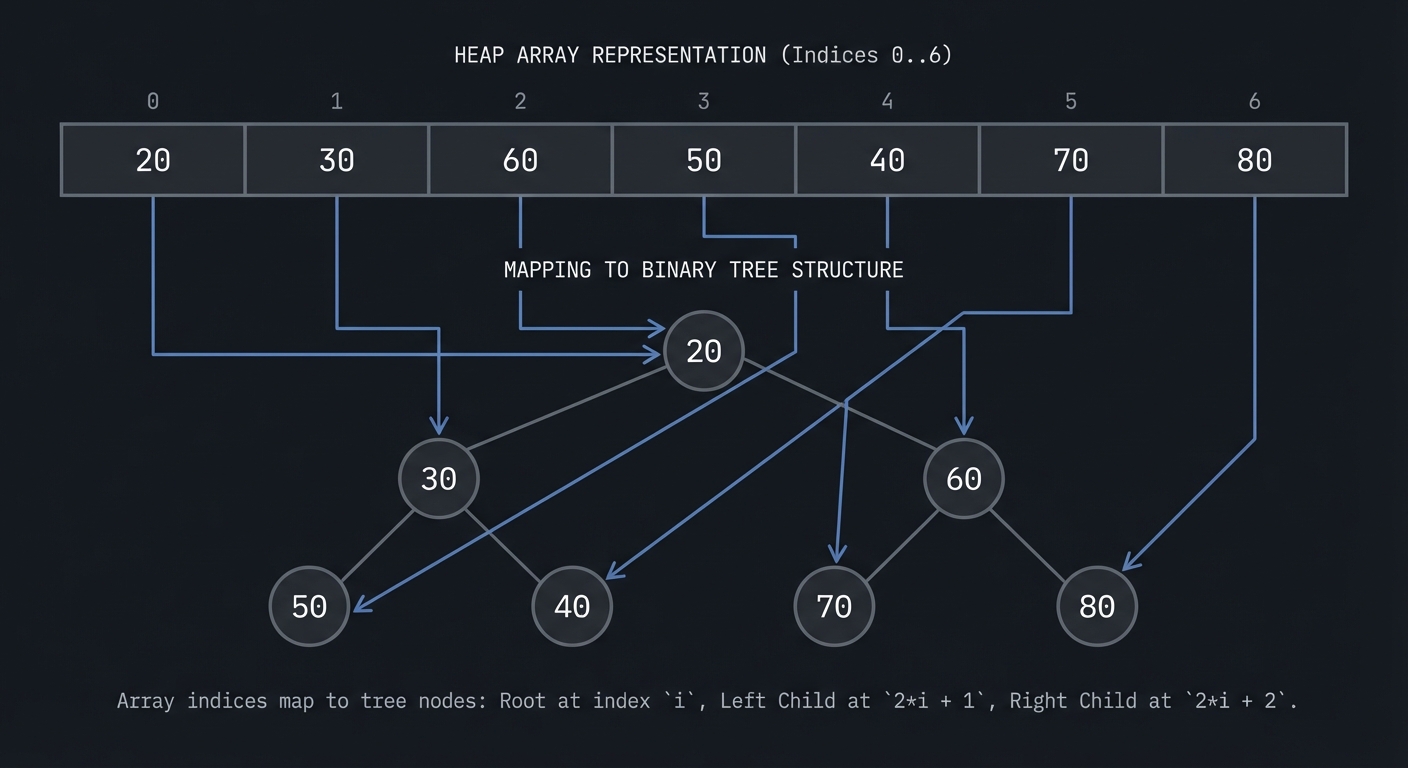
Heap vs BST vs Sorted Array

Operation	Heap	BST (balanced)	Sorted Array
Find min/max	O(1)	O(log n)	O(1)
Insert	O(log n)	O(log n)	O(n)
Extract min/max	O(log n)	O(log n)	O(1) or O(n)
Build from array	O(n)	O(n log n)	O(n log n)
Find arbitrary	O(n)	O(log n)	O(log n)
Memory	Minimal (array)	Pointers overhead	Minimal

Use Heap when:

• You only need min or max, not both
• Priority queue operations
• Heapsort (in-place)

---

Project 8: Graph Algorithms Visualizer

• Main Programming Language: C
• Alternative Programming Languages: Rust, Python, JavaScript
• Coolness Level: Level 5: Pure Magic (Super Cool)
• Business Potential: 1. The “Resume Gold”
• Difficulty: Level 4: Expert
• Knowledge Area: Graphs / Algorithms
• Software or Tool: Terminal/ncurses visualizer
• Main Book: Introduction to Algorithms by CLRS

What you’ll build

A graph library with visualization that demonstrates BFS, DFS, Dijkstra’s shortest path, and topological sort—showing how graphs model real-world relationships.

Deliverables:

• graph.c/.h with adjacency list/matrix support
• BFS/DFS/Dijkstra/topo sort demos
• Visualization output for small graphs

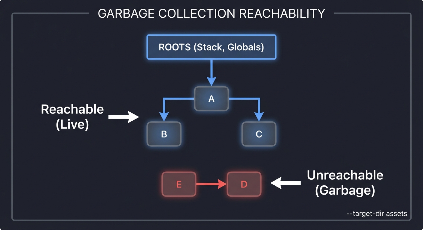
Why it teaches this concept

Graphs are everywhere:

• Social networks (people and friendships)
• Maps (cities and roads)
• The internet (pages and links)
• Dependencies (packages, tasks)
• Neural networks

Understanding graphs unlocks:

• Shortest path (GPS navigation)
• Social network analysis
• Dependency resolution (npm, cargo)
• Web crawling
• Recommendation systems

Graphs are the most general structure: many problems become graph problems once you model relationships.

Core challenges you’ll face

• Graph representation (adjacency list vs matrix) → maps to space/time trade-off
• BFS (shortest path in unweighted graphs) → maps to level-order
• DFS (explore deeply, backtrack) → maps to stack/recursion
• Dijkstra’s (shortest path with weights) → maps to greedy + heap
• Topological sort (ordering with dependencies) → maps to DAGs
• Edge weighting (positive weights only for Dijkstra) → maps to constraints

Resources for Key Challenges

• GeeksforGeeks: Real-life Applications of DSA - Graphs in maps, networks
• FreeCodeCamp: Real-world data structures - Graph applications

Key Concepts

Concept	Resource
Graph Representations	Introduction to Algorithms Chapter 22 - CLRS
BFS/DFS	Introduction to Algorithms Chapter 22.2-22.3 - CLRS
Dijkstra’s Algorithm	Introduction to Algorithms Chapter 24.3 - CLRS
Topological Sort	Introduction to Algorithms Chapter 22.4 - CLRS
Graph APIs in C	Algorithms in C, Parts 1-4

Difficulty & Time

• Difficulty: Advanced
• Time estimate: 2 weeks
• Prerequisites: Projects 1-7 completed, especially heap
• Stretch goal: Add A* pathfinding

Real World Outcome

$ ./graph_demo

=== Graph Representation ===
Creating a city road network...

Adjacency List:
  NYC -> [Boston(215), Philadelphia(97)]
  Boston -> [NYC(215), Portland(108)]
  Philadelphia -> [NYC(97), DC(140)]
  DC -> [Philadelphia(140), Richmond(109)]
  Portland -> [Boston(108)]
  Richmond -> [DC(109)]

Adjacency Matrix:
           NYC  BOS  PHL  DC   PRT  RCH
    NYC     0   215   97   0    0    0
    BOS   215    0    0    0   108   0
    PHL    97    0    0   140   0    0
    DC      0    0   140   0    0   109
    PRT     0   108   0    0    0    0
    RCH     0    0    0   109   0    0

=== BFS: Shortest Path (unweighted) ===
From NYC, how many hops to each city?

         NYC
         /  \
      BOS   PHL
       |      \
     PRT      DC
               |
             RCH

Distances: NYC(0) BOS(1) PHL(1) DC(2) PRT(2) RCH(3)

=== DFS: Explore Deeply ===
Starting from NYC...
Visit order: NYC -> Boston -> Portland -> (backtrack) ->
             Philadelphia -> DC -> Richmond

=== Dijkstra: Shortest Path (weighted) ===
Shortest path from NYC to Richmond:

Step 1: Process NYC, update neighbors
  Boston: ∞ -> 215, Philadelphia: ∞ -> 97
Step 2: Process Philadelphia (closest), update neighbors
  DC: ∞ -> 237
Step 3: Process Boston, update neighbors
  Portland: ∞ -> 323
Step 4: Process DC, update neighbors
  Richmond: ∞ -> 346
Step 5: Process Portland (no new paths)
Step 6: Process Richmond (destination!)

Shortest path NYC -> Richmond: 346 miles
Route: NYC -> Philadelphia -> DC -> Richmond

=== Topological Sort: Task Dependencies ===
Build system dependencies:
  main.c depends on: utils.h, config.h
  utils.c depends on: utils.h
  config.c depends on: config.h
  program depends on: main.o, utils.o, config.o

Valid build order:
  1. config.h
  2. utils.h
  3. config.c -> config.o
  4. utils.c -> utils.o
  5. main.c -> main.o
  6. program

You should be able to explain why adjacency lists are better for sparse graphs.

The Core Question You’re Answering

How do you model relationships between entities and compute reachability, shortest paths, and valid execution order? Which graph representation makes your operations fastest?

Concepts You Must Understand First

• Graph representations (CLRS, Ch 22)
• BFS and DFS correctness (CLRS, Ch 22.2-22.3)
• Dijkstra’s algorithm (CLRS, Ch 24.3)
• Topological sorting (CLRS, Ch 22.4)
• Priority queues for shortest path (CLRS, Ch 6.5)

Questions to Guide Your Design

• Should you use adjacency lists or matrices for your graph size?
• How will you store edge weights and directionality?
• How will you visualize traversal to debug it?
• How will you detect cycles for topological sort?
• How will you represent disconnected components?

Thinking Exercise

Draw a small directed graph of 5 nodes with a cycle. Try to topologically sort it and observe why it fails. Now remove one edge and try again.

The Interview Questions They’ll Ask

• When is BFS preferred over DFS?
• Why does Dijkstra fail with negative weights?
• How do you detect cycles in a graph?
• What is the complexity of adjacency list vs matrix?
• How do you store a sparse graph efficiently?
• What is the difference between DAG and tree?

Hints in Layers

1) Implement adjacency list for sparse graphs. 2) Build BFS and DFS with explicit visited tracking. 3) Add Dijkstra with a priority queue for performance. 4) Implement Kahn’s algorithm for topological sort. 5) Add a graph_validate() function that checks edge consistency.

visited[start] = 1;
queue[rear++] = start;
while (front < rear) {
    int v = queue[front++];
    // explore neighbors
}

Books That Will Help

Topic	Book	Why It Helps
Graph basics	CLRS, Ch 22	Core algorithms
Shortest path	CLRS, Ch 24	Dijkstra details
Graphs in C	Algorithms in C, Parts 1-4	Implementation patterns
Visual intuition	Graph Algorithms the Fun Way	Step-by-step reasoning

Common Pitfalls & Debugging

Problem: “DFS misses nodes”

• Why: Visited not tracked or reset.
• Fix: Initialize visited array and set on entry.
• Quick test: Run DFS on disconnected graph and confirm all components.

Problem: “Dijkstra gives wrong path”

• Why: Priority queue not updated or negative edge weight used.
• Fix: Reject negative weights and update distances properly.
• Quick test: Compare against known shortest path on a small graph.

Problem: “Topological sort outputs fewer nodes”

• Why: Cycle exists or in-degree updates are wrong.
• Fix: Validate in-degree updates and detect cycles.
• Quick test: Run on a DAG and a cyclic graph.

Problem: “Adjacency matrix wastes memory”

• Why: Using matrix for sparse graph.
• Fix: Switch to adjacency list for large, sparse graphs.
• Quick test: Compare memory usage for V=10,000.

Definition of Done

• Graph supports both directed and undirected edges
• BFS and DFS produce correct visitation order
• Dijkstra returns correct shortest path and distance
• Topological sort detects cycles and orders DAGs
• Visualization makes traversal steps obvious
• Complexity notes included in README

Learning Milestones

1. Can create graphs both ways → You understand representation trade-offs
2. BFS finds shortest unweighted path → You understand level-order
3. DFS explores deeply → You understand backtracking
4. Dijkstra’s with heap works → You understand greedy algorithms
5. Topological sort orders dependencies → You understand DAGs
6. Complexities match theory → You can reason about O(V+E)

Implementation

Graph Representation

// Adjacency List (better for sparse graphs)
typedef struct Edge {
    int destination;
    int weight;
    struct Edge* next;
} Edge;

typedef struct {
    Edge** adj_list;  // Array of linked lists
    int num_vertices;
    int is_directed;
} Graph;

Graph* graph_create(int vertices, int is_directed) {
    Graph* g = malloc(sizeof(Graph));
    g->num_vertices = vertices;
    g->is_directed = is_directed;
    g->adj_list = calloc(vertices, sizeof(Edge*));
    return g;
}

void graph_add_edge(Graph* g, int src, int dest, int weight) {
    Edge* edge = malloc(sizeof(Edge));
    edge->destination = dest;
    edge->weight = weight;
    edge->next = g->adj_list[src];
    g->adj_list[src] = edge;

    if (!g->is_directed) {
        Edge* reverse = malloc(sizeof(Edge));
        reverse->destination = src;
        reverse->weight = weight;
        reverse->next = g->adj_list[dest];
        g->adj_list[dest] = reverse;
    }
}

BFS (Breadth-First Search)

void bfs(Graph* g, int start) {
    int* visited = calloc(g->num_vertices, sizeof(int));
    int* distance = malloc(g->num_vertices * sizeof(int));
    for (int i = 0; i < g->num_vertices; i++) {
        distance[i] = -1;
    }

    // Queue
    int* queue = malloc(g->num_vertices * sizeof(int));
    int front = 0, rear = 0;

    visited[start] = 1;
    distance[start] = 0;
    queue[rear++] = start;

    printf("BFS from vertex %d:\n", start);

    while (front < rear) {
        int current = queue[front++];
        printf("  Visit %d (distance %d)\n", current, distance[current]);

        Edge* edge = g->adj_list[current];
        while (edge) {
            if (!visited[edge->destination]) {
                visited[edge->destination] = 1;
                distance[edge->destination] = distance[current] + 1;
                queue[rear++] = edge->destination;
            }
            edge = edge->next;
        }
    }

    free(visited);
    free(distance);
    free(queue);
}

DFS (Depth-First Search)

void dfs_helper(Graph* g, int vertex, int* visited) {
    visited[vertex] = 1;
    printf("  Visit %d\n", vertex);

    Edge* edge = g->adj_list[vertex];
    while (edge) {
        if (!visited[edge->destination]) {
            dfs_helper(g, edge->destination, visited);
        }
        edge = edge->next;
    }

    printf("  Backtrack from %d\n", vertex);
}

void dfs(Graph* g, int start) {
    int* visited = calloc(g->num_vertices, sizeof(int));
    printf("DFS from vertex %d:\n", start);
    dfs_helper(g, start, visited);
    free(visited);
}

Dijkstra’s Algorithm (with Min-Heap)

typedef struct {
    int vertex;
    int distance;
} HeapNode;

void dijkstra(Graph* g, int start, int* dist, int* prev) {
    // Initialize distances
    for (int i = 0; i < g->num_vertices; i++) {
        dist[i] = INT_MAX;
        prev[i] = -1;
    }
    dist[start] = 0;

    // Min-heap priority queue
    HeapNode* heap = malloc(g->num_vertices * sizeof(HeapNode));
    int heap_size = 0;

    // Insert start
    heap[heap_size++] = (HeapNode){start, 0};

    int* processed = calloc(g->num_vertices, sizeof(int));

    while (heap_size > 0) {
        // Extract min (simplified - should use proper heap)
        int min_idx = 0;
        for (int i = 1; i < heap_size; i++) {
            if (heap[i].distance < heap[min_idx].distance) {
                min_idx = i;
            }
        }

        HeapNode current = heap[min_idx];
        heap[min_idx] = heap[--heap_size];

        if (processed[current.vertex]) continue;
        processed[current.vertex] = 1;

        printf("Process vertex %d (distance %d)\n",
               current.vertex, current.distance);

        // Update neighbors
        Edge* edge = g->adj_list[current.vertex];
        while (edge) {
            int new_dist = dist[current.vertex] + edge->weight;
            if (new_dist < dist[edge->destination]) {
                dist[edge->destination] = new_dist;
                prev[edge->destination] = current.vertex;
                heap[heap_size++] = (HeapNode){edge->destination, new_dist};
                printf("  Update %d: distance = %d\n",
                       edge->destination, new_dist);
            }
            edge = edge->next;
        }
    }

    free(heap);
    free(processed);
}

void print_path(int* prev, int dest) {
    if (prev[dest] != -1) {
        print_path(prev, prev[dest]);
        printf(" -> ");
    }
    printf("%d", dest);
}

Topological Sort (Kahn’s Algorithm)

void topological_sort(Graph* g) {
    int* in_degree = calloc(g->num_vertices, sizeof(int));

    // Calculate in-degrees
    for (int v = 0; v < g->num_vertices; v++) {
        Edge* edge = g->adj_list[v];
        while (edge) {
            in_degree[edge->destination]++;
            edge = edge->next;
        }
    }

    // Queue of vertices with in-degree 0
    int* queue = malloc(g->num_vertices * sizeof(int));
    int front = 0, rear = 0;

    for (int v = 0; v < g->num_vertices; v++) {
        if (in_degree[v] == 0) {
            queue[rear++] = v;
        }
    }

    printf("Topological order: ");
    int count = 0;

    while (front < rear) {
        int current = queue[front++];
        printf("%d ", current);
        count++;

        Edge* edge = g->adj_list[current];
        while (edge) {
            in_degree[edge->destination]--;
            if (in_degree[edge->destination] == 0) {
                queue[rear++] = edge->destination;
            }
            edge = edge->next;
        }
    }

    if (count != g->num_vertices) {
        printf("\nCycle detected! Not a DAG.\n");
    }
    printf("\n");

    free(in_degree);
    free(queue);
}

Design Notes

• Use adjacency lists for sparse graphs and matrices for dense graphs.
• Keep graph directed/undirected as a flag in the graph struct.
• Always validate vertex bounds when adding edges.
• For Dijkstra, use a proper min-heap instead of linear scan.

Testing & Validation

• Run BFS/DFS on disconnected graphs and verify full coverage.
• Validate Dijkstra on a small weighted graph with known distances.
• Test topological sort on DAGs and graphs with cycles.

Performance Experiments

• Compare adjacency list vs matrix memory for V=10,000 and E=20,000.
• Benchmark BFS on sparse vs dense graphs.
• Measure Dijkstra performance with and without a heap.

Adjacency List vs Matrix (example graph)

List:
0 -> 1, 2
1 -> 2
2 -> 0

Matrix:
   0 1 2
0 [0 1 1]
1 [0 0 1]
2 [1 0 0]

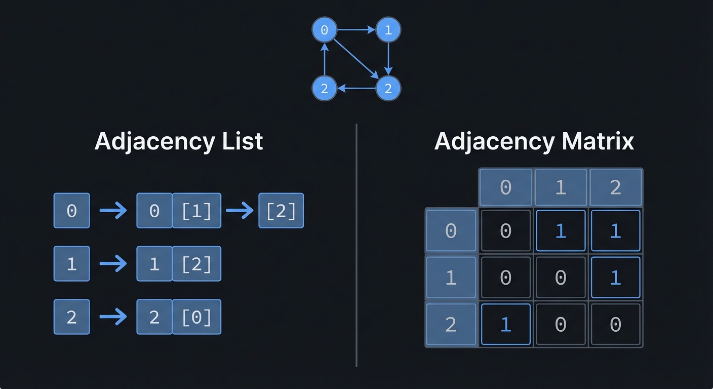
Adjacency List vs Adjacency Matrix

Aspect	Adjacency List	Adjacency Matrix
Space	O(V + E)	O(V²)
Check if edge exists	O(degree)	O(1)
Find all neighbors	O(degree)	O(V)
Add edge	O(1)	O(1)
Best for	Sparse graphs	Dense graphs

---

Project 9: Mini Database Engine (Capstone)

• Main Programming Language: C
• Alternative Programming Languages: Rust, C++
• Coolness Level: Level 5: Pure Magic (Super Cool)
• Business Potential: 4. The “Open Core” Infrastructure
• Difficulty: Level 5: Master
• Knowledge Area: Databases / Systems Programming
• Software or Tool: SQL-like query engine
• Main Book: Database Internals by Alex Petrov

What you’ll build

A mini database that combines everything you’ve learned: B-tree indexing, hash tables for lookups, heaps for sorting, and more—with a simple SQL-like query language.

Deliverables:

• storage.c for page management
• btree.c and hash_index.c
• parser.c for a tiny SQL-like grammar
• CLI with EXPLAIN and STATS

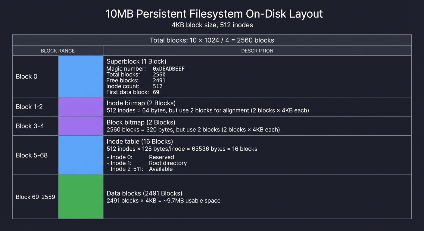
Why this is the capstone

Real databases are the ultimate data structure application:

• Hash indexes for equality lookups
• B-trees for range queries
• Heaps for sorting and top-k
• Graphs for query planning

Building a mini database proves you understand when to use each structure.

B-trees are especially critical because they reduce tree height by packing many keys into one node, minimizing disk I/O.

Source: https://en.wikipedia.org/wiki/B-tree

Core challenges you’ll face

• Storage engine (pages, buffer pool) → maps to memory management
• B-tree index (balanced tree for disk) → maps to tree structures
• Hash index (fast equality lookup) → maps to hash tables
• Query execution (scans, filters, joins) → maps to algorithm design
• Query parsing (SQL-like syntax) → maps to stack machines
• On-disk layout (pages, slots) → maps to physical design

Key Concepts

Concept	Resource
B-Trees	Introduction to Algorithms Chapter 18 - CLRS
Database Storage	Database Internals Chapters 1-4 - Alex Petrov
Query Processing	Database System Concepts Chapter 12 - Silberschatz
Buffer Management	Database Internals Chapter 5 - Alex Petrov
Index maintenance	Database System Concepts Chapter 11

Difficulty & Time

• Difficulty: Expert/Master
• Time estimate: 4-6 weeks
• Prerequisites: All previous projects completed
• Stretch goal: Add a simple join operator

Real World Outcome

$ ./minidb

MiniDB v1.0 - A learning database engine
Type 'help' for commands.

minidb> CREATE TABLE users (id INT, name TEXT, age INT);
Table 'users' created.

minidb> CREATE INDEX idx_id ON users(id) USING HASH;
Hash index 'idx_id' created on users(id).

minidb> CREATE INDEX idx_age ON users(age) USING BTREE;
B-tree index 'idx_age' created on users(age).

minidb> INSERT INTO users VALUES (1, 'Alice', 30);
INSERT INTO users VALUES (2, 'Bob', 25);
INSERT INTO users VALUES (3, 'Charlie', 35);
Inserted 3 rows.

minidb> SELECT * FROM users;
+----+---------+-----+
| id | name    | age |
+----+---------+-----+
| 1  | Alice   | 30  |
| 2  | Bob     | 25  |
| 3  | Charlie | 35  |
+----+---------+-----+
3 rows returned (full table scan)

minidb> SELECT * FROM users WHERE id = 2;
+----+------+-----+
| id | name | age |
+----+------+-----+
| 2  | Bob  | 25  |
+----+------+-----+
1 row returned (used hash index 'idx_id')

minidb> SELECT * FROM users WHERE age > 28 ORDER BY age;
+----+---------+-----+
| id | name    | age |
+----+---------+-----+
| 1  | Alice   | 30  |
| 3  | Charlie | 35  |
+----+---------+-----+
2 rows returned (used B-tree index 'idx_age' for range scan)

minidb> EXPLAIN SELECT * FROM users WHERE age > 28;
Query Plan:
  -> Index Range Scan on idx_age (age > 28)
     -> Fetch rows from table 'users'
        -> Return results

minidb> .stats
Database Statistics:
  Tables: 1
  Total rows: 3
  Hash indexes: 1 (idx_id)
  B-tree indexes: 1 (idx_age)
  Buffer pool: 16 pages, 2 dirty

minidb> .dump users
Page 0: [1|Alice|30] [2|Bob|25] [3|Charlie|35]
B-tree idx_age:
        [30]
       /    \
    [25]    [35]

You should be able to show which index is used for a query and why that plan is better than a full scan.

The Core Question You’re Answering

How do real databases combine multiple data structures to handle storage, indexing, and query execution efficiently? Which structure dominates which query shape?

Concepts You Must Understand First

• On-disk pages and buffer pools (Database Internals, Ch 1-4)
• B-tree invariants and splits (CLRS, Ch 18)
• Hash indexes for equality lookup (CLRS, Ch 11)
• Query execution basics (Database System Concepts, Ch 12)
• Disk latency vs memory latency (see latency section above)

Questions to Guide Your Design

• What is the page size and how do you pack rows into pages?
• How will you represent and update a B-tree node on disk?
• When should you use a hash index vs a B-tree index?
• How will you implement a simple query planner?
• How will you keep indexes consistent after deletes?

Thinking Exercise

Sketch a table with 3 pages and 20 rows. Decide which rows live on which page, then simulate a range query with a B-tree index. Count the number of page reads.

The Interview Questions They’ll Ask

• Why are B-trees preferred for disk-based indexes?
• What is a buffer pool and why does it need eviction?
• How does an index scan differ from a full table scan?
• What is the difference between a heap file and an index?
• How do you keep indexes consistent during inserts?
• What is the write amplification trade-off of indexes?

Hints in Layers

1) Start with in-memory rows and a simple scan-based query engine. 2) Add a hash index for equality lookups. 3) Implement a B-tree for range queries. 4) Add an EXPLAIN output to show the chosen plan. 5) Add basic stats (row counts, index sizes).

if (op == EQ && has_hash_index(column)) use_hash();
else if ((op == GT || op == LT) && has_btree_index(column)) use_btree();
else full_scan();

Books That Will Help

Topic	Book	Why It Helps
Database internals	Database Internals, Ch 1-4	Storage engine concepts
B-trees	CLRS, Ch 18	B-tree algorithms
Query processing	Database System Concepts, Ch 12	Planner and execution
Indexing basics	Database System Concepts, Ch 11	Index maintenance

Common Pitfalls & Debugging

Problem: “Index returns wrong rows”

• Why: Index not updated after insert/delete.
• Fix: Update index during every row mutation.
• Quick test: Insert rows, then query by index and by full scan.

Problem: “B-tree split loses keys”

• Why: Incorrect split point or child reassignment.
• Fix: Follow a strict split procedure and test with small trees.
• Quick test: Insert keys 1..20 and verify in-order traversal.

Problem: “Query planner always uses full scan”

• Why: Missing stats or index detection logic.
• Fix: Track index existence and column selectivity.
• Quick test: Compare EXPLAIN output for indexed vs non-indexed queries.

Problem: “Pages overlap or corrupt”

• Why: Off-by-one in page offset math.
• Fix: Use fixed page sizes and validate offsets.
• Quick test: Insert rows until a new page is allocated and verify boundaries.

Definition of Done

• MiniDB can create tables, insert rows, and query data
• Hash index speeds up equality queries
• B-tree index supports range scans
• EXPLAIN shows chosen plan and index usage
• Basic stats and page dumps work correctly
• Indexes remain consistent after deletes

Learning Milestones

1. Can store and retrieve rows → You understand storage
2. Hash index speeds up equality queries → You understand hash tables in practice
3. B-tree index enables range queries → You understand balanced trees in practice
4. Query planner chooses correct index → You understand optimization
5. Page layout is consistent → You understand persistence

Architecture Overview

┌────────────────────────────────────────────────────────────────┐
│                         MiniDB                                  │
├────────────────────────────────────────────────────────────────┤
│  ┌──────────────┐  ┌──────────────┐  ┌──────────────────────┐ │
│  │ SQL Parser   │  │ Query        │  │ Query Executor       │ │
│  │              │→ │ Planner      │→ │                      │ │
│  │ (Stack-based)│  │ (Choose idx) │  │ (Scan/Filter/Sort)  │ │
│  └──────────────┘  └──────────────┘  └──────────────────────┘ │
│                                              │                  │
│                                              ▼                  │
│  ┌──────────────────────────────────────────────────────────┐ │
│  │                    Index Manager                          │ │
│  │  ┌─────────────┐  ┌─────────────┐  ┌─────────────────┐  │ │
│  │  │ Hash Index  │  │ B-Tree Index│  │ (future: R-tree)│  │ │
│  │  │  O(1) ==    │  │ O(log n) <> │  │                 │  │ │
│  │  └─────────────┘  └─────────────┘  └─────────────────┘  │ │
│  └──────────────────────────────────────────────────────────┘ │
│                                              │                  │
│                                              ▼                  │
│  ┌──────────────────────────────────────────────────────────┐ │
│  │                   Storage Engine                          │ │
│  │  ┌─────────────┐  ┌─────────────┐  ┌─────────────────┐  │ │
│  │  │ Buffer Pool │  │ Page Manager│  │ Heap File       │  │ │
│  │  │ (LRU Cache) │  │ (Slotted)   │  │ (Row Storage)   │  │ │
│  │  └─────────────┘  └─────────────┘  └─────────────────┘  │ │
│  └──────────────────────────────────────────────────────────┘ │
│                                              │                  │
│                                              ▼                  │
│  ┌──────────────────────────────────────────────────────────┐ │
│  │                    Disk (Files)                           │ │
│  │  [users.dat] [users_idx_id.hash] [users_idx_age.btree]   │ │
│  └──────────────────────────────────────────────────────────┘ │
└────────────────────────────────────────────────────────────────┘

Implementation Skeleton

// Row storage
typedef struct {
    int id;
    char name[64];
    int age;
} Row;

// Table metadata
typedef struct {
    char name[64];
    int num_rows;
    Row* rows;  // Simple in-memory for now
    HashTable* hash_indexes;
    BTree* btree_indexes;
} Table;

// Database
typedef struct {
    Table* tables[MAX_TABLES];
    int num_tables;
} Database;

// Query result
typedef struct {
    Row* rows;
    int count;
    char index_used[64];
} QueryResult;

// Execute SELECT with index selection
QueryResult* execute_select(Table* table, const char* column,
                           const char* op, int value) {
    QueryResult* result = malloc(sizeof(QueryResult));
    result->rows = malloc(table->num_rows * sizeof(Row));
    result->count = 0;

    // Check for applicable index
    if (strcmp(op, "=") == 0 && has_hash_index(table, column)) {
        // Use hash index for O(1) lookup
        int* row_ids = hash_index_lookup(table, column, value);
        strcpy(result->index_used, "hash");
        // Fetch rows...
    }
    else if ((strcmp(op, ">") == 0 || strcmp(op, "<") == 0) &&
             has_btree_index(table, column)) {
        // Use B-tree for range scan
        int* row_ids = btree_range_scan(table, column, op, value);
        strcpy(result->index_used, "btree");
        // Fetch rows...
    }
    else {
        // Full table scan
        strcpy(result->index_used, "none (full scan)");
        for (int i = 0; i < table->num_rows; i++) {
            if (matches_condition(&table->rows[i], column, op, value)) {
                result->rows[result->count++] = table->rows[i];
            }
        }
    }

    return result;
}

Design Notes

• Pick a fixed page size (e.g., 4KB) and never deviate.
• Keep B-tree nodes sized to fit in a page to reduce I/O.
• Separate storage from indexing to keep code modular.
• Always update indexes on insert/delete to avoid stale entries.

Testing & Validation

• Insert rows until you trigger B-tree splits, then verify in-order traversal.
• Verify that hash index returns the same results as a full scan.
• Run crash-restart simulation by saving pages and reloading.

Performance Experiments

• Compare full scan vs index scan latency on increasing data sizes.
• Measure how many pages are read for range queries.
• Track buffer pool hit rate under repeated workloads.

B-tree Page Layout (simplified)

[Header | KeyCount=3 | P0 | K1 | P1 | K2 | P2 | K3 | P3 | Free]
          ^ keys and child pointers packed in page

---

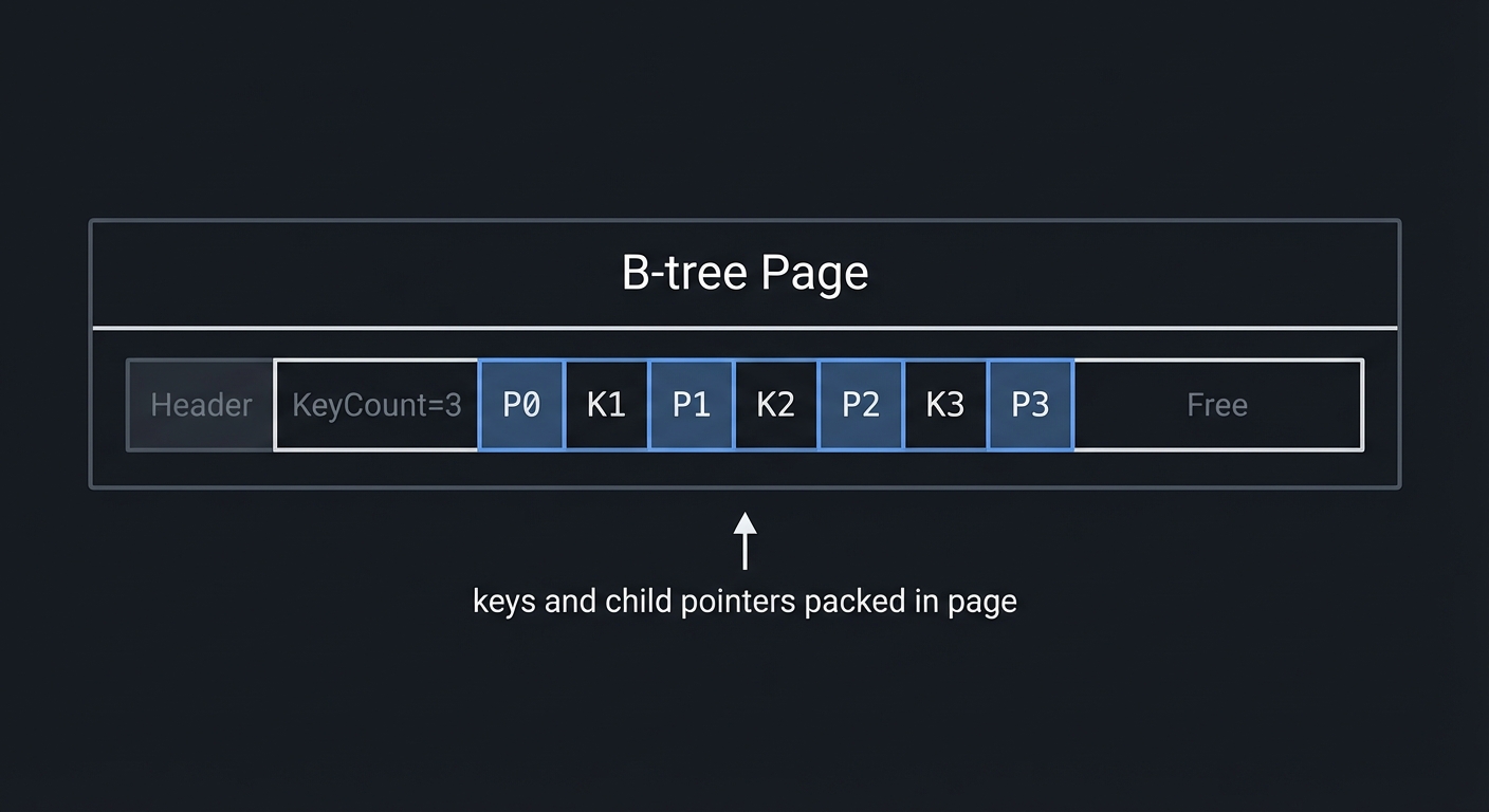
Mini-Lab Appendix (Benchmarks & Debug Tasks)

These labs are short, repeatable exercises to validate correctness and performance. Keep results in a labs.md file.

Lab 1: Memory Arena & Dynamic Array

• Benchmark: Push 1M integers; record total reallocations and runtime.
• Profile: Compare iteration time for array vs list (same data).
• Debug: Intentionally trigger an out-of-memory condition and handle it cleanly.

Lab 2: Linked List Toolkit

• Benchmark: Insert/delete 100k nodes at head vs tail and compare.
• Profile: Measure traversal time with perf or Instruments.
• Debug: Introduce a cycle, then detect and remove it.

Lab 3: Stack Machine

• Benchmark: Evaluate a long RPN expression (10k tokens).
• Profile: Compare fixed-size stack vs dynamic stack.
• Debug: Fuzz tokens and ensure errors are handled without crashes.

Lab 4: Queue Systems

• Benchmark: Enqueue/dequeue 1M ops in a ring buffer.
• Profile: Compare queue vs array-shift implementation.
• Debug: Prove BFS path length equals distance array output.

Lab 5: Hash Table

• Benchmark: Insert 1M keys and measure average probe length.
• Profile: Compare chaining vs open addressing at different load factors.
• Debug: Verify all keys remain after a resize.

Lab 6: BST & Balancing

• Benchmark: Insert sorted vs random data; record tree height.
• Profile: Measure search time for balanced vs unbalanced trees.
• Debug: Validate all four AVL rotation cases.

Lab 7: Heap & Priority Queue

• Benchmark: Build heap from array vs repeated inserts.
• Profile: Compare binary heap vs 4-ary heap for Dijkstra-like workloads.
• Debug: Verify heap property after each extract.

Lab 8: Graph Algorithms

• Benchmark: Run BFS/DFS on sparse vs dense graphs.
• Profile: Compare adjacency list vs matrix memory.
• Debug: Detect cycles and verify topological sort output size.

Lab 9: Mini Database

• Benchmark: Compare full scan vs index scan over 100k rows.
• Profile: Track buffer pool hit ratio under repeated queries.
• Debug: Verify B-tree splits preserve in-order traversal.

---

Essential Resources Summary

Primary Books (in order)

1. Introduction to Algorithms (CLRS) - The bible of algorithms and data structures
2. Algorithms, Fourth Edition by Sedgewick - More accessible, excellent visualizations
3. Computer Systems: A Programmer’s Perspective - For understanding memory
4. Grokking Algorithms - Visual, beginner-friendly
5. Database Internals by Alex Petrov - For the capstone project
6. Algorithms in C, Parts 1-4 by Sedgewick - C implementations and patterns

From Your Library

• C Programming: A Modern Approach by K.N. King - For implementation
• The C Programming Language by K&R - Reference
• Data Structures the Fun Way by Jeremy Kubica - Visual learning
• Grokking Data Structures by Marcello La Rocca - Beginner-friendly
• Advanced Algorithms and Data Structures by Marcello La Rocca - Advanced topics
• Mastering Algorithms with C by Kyle Loudon - Practical C data structures

Online Resources

• Visualgo.net - Animated data structure visualizations
• GeeksforGeeks: Real-life Applications - Practical examples
• The Lost Art of Structure Packing - Memory layout optimization
• CLRS lecture notes (MIT OCW) - Algorithm explanations

---

The Big Picture: When to Use What

I Need To…	Use This	Why
Access by index	Array	O(1) random access
Insert/delete frequently at ends	Linked List	O(1) with pointers
LIFO (last in, first out)	Stack	O(1) push/pop
FIFO (first in, first out)	Queue	O(1) enqueue/dequeue
Fast lookup by key	Hash Table	O(1) average
Ordered data + fast search	BST / B-Tree	O(log n) everything
Fast min/max only	Heap	O(1) peek, O(log n) extract
Model relationships	Graph	Represents connections
Combine multiple needs	Custom	e.g., LRU = Hash + DLL
Frequent range queries	B-tree	Disk-friendly ordering
High update rates with sequential writes	Log-structured (LSM)	Writes are fast, reads use compaction

---

Appendix: Complexity Cheat Sheet

Data Structure	Access	Search	Insert	Delete	Space
Array	O(1)	O(n)	O(n)	O(n)	O(n)
Dynamic Array	O(1)	O(n)	O(1)*	O(n)	O(n)
Linked List	O(n)	O(n)	O(1)†	O(1)†	O(n)
Stack	O(n)	O(n)	O(1)	O(1)	O(n)
Queue	O(n)	O(n)	O(1)	O(1)	O(n)
Hash Table	N/A	O(1)*	O(1)*	O(1)*	O(n)
BST (balanced)	O(log n)	O(log n)	O(log n)	O(log n)	O(n)
BST (unbalanced)	O(n)	O(n)	O(n)	O(n)	O(n)
Heap	O(1)‡	O(n)	O(log n)	O(log n)	O(n)
Graph (adj list)	O(V)	O(V)	O(1)	O(E)	O(V+E)

*amortized †if you have the pointer ‡min/max only

Remember: these are asymptotic costs. Real performance depends on cache locality, constant factors, and memory layout.